Worcester Polytechnic Institute
Digital WPI
Interactive Qualifying Projects (All Years) Interactive Qualifying Projects
March 2019
Stock Market Prediction
Nolan Woodie Greig
Worcester Polytechnic Institute
Talal A. Jaber
Worcester Polytechnic Institute
Follow this and additional works at:https://digitalcommons.wpi.edu/iqp-all
This Unrestricted is brought to you for free and open access by the Interactive Qualifying Projects at Digital WPI. It has been accepted for inclusion in Interactive Qualifying Projects (All Years) by an authorized administrator of Digital WPI. For more information, please [email protected].
Repository Citation
Models for the Prediction of Individual Stock Prices
An Interactive Qualifying Project submitted to the Faculty of
WORCESTER POLYTECHNIC INSTITUTE in partial fulfilment of the requirements for the
degree of Bachelor of Science by Nolan Greig Talal Jaber Date: 1 March 2019
Report Submitted to:
Mayer Humi, PhD Worcester Polytechnic Institute
Abstract
This project aims to predict the price of a stock using MATLAB. The model is designed to predict the price of mid-priced stocks ($20-200) over a short (2-3 week) timeframe. Different methods of filtering and weighting the data are tested to improve the length of the prediction. Furthermore, a virtual stock portfolio was created and analyzed over 7 weeks.
Table of Contents
Abstract 3
Table of Contents 4
Executive Summary 5
Introduction 6
Data Analysis & Improvisation 7
1) Prototype Model 8
2) Moving Average Model 14
3) Stock Index Cross Correlation Model 17
4) Fast Fourier Transform and Stock Index Cross Correlation Model 19
Simulated Market Portfolio 21
Results 22
1) Prototype Model 22
2) Moving Average Model 23
3) Stock Index Cross Correlation Model 24
4) Fast Fourier Transform and Stock Index Cross Correlation Model 26
Virtual Portfolio 1 27
Virtual Portfolio 2 32
Summary 36
Recommendations 37
Executive Summary
First, each of us selected a number of stocks in a specific segment of the market. The stocks were chosen to be in reach for an “average” trader (priced between $20 and $200) and that would be a good candidate for investing. 10 stocks from the construction segment and 10 from the technology were chosen to be tested upon and learned from. The reasoning behind choosing these specific sectors was that they corresponded to our studies and thus, were easier to research and evaluate. Later, 5 more stocks from each segment were added to the list, as an assurance that our findings were applicable to a wide variety of stocks.
From here, a prototype for predicting the price of the stock was developed. The historical closing price of each stock from Sep 05 2017 to Sep 05 2018 was downloaded. For the purposes of the project, Sep 05 2018 was chosen to act as the present day for any predictions. Using our models, we attempted to generate predictions of the stocks’ prices up to 17 business days after this date, and compared these predictions with the actual stock prices. This limit of 17 business days was determined due to the majority of predictions turning invalid within that period of time.
As a first step towards the building of the prototype model for individual stock, we computed an autocorrelation of the historical data of the stock. The first zero-valued lag was taken as the period of relevant data for the stock. This period (starting from the present) was used to create a line portraying the least squares fit (stock trend price). This trendline was subtracted from the historical data to center the data on the x-axis. A Fourier series was fit to this data with
a number of terms based on the period of the autocorrelation. The prediction was created by adding the trendline to the Fourier series. An error band was created by averaging the minimum and maximum error between the prediction and the historical data. The prediction and error band were then extended into the future and compared with the actual stock price data.
A number of models were used in an attempt to improve this preliminary model. Moving averages were used to smooth the historical data. The FFT algorithm was also used to smooth the data. Finally, stock indices such as the Dow Jones Industrial average were correlated with the prediction for the stock. The coefficients of this correlation were used to weight the predictions and improve the prediction.
As an evaluation of the project, each of us participated in a 7 week simulated version of the stock market. Using the model created as well as any other information, statistics or analyses deemed relevant, each of us chose 10 stocks based on their predicted ability to turn a profit in 7 weeks. For the sake of the simulation, we stated with $100,000 and split the money between stocks as we saw fit. Every week, we monitored the progress of the portfolio and evaluated the performance of each stock.
Introduction
The stock market today is dominated by huge players that use sophisticated modeling and prediction tools backed up by a large number of professionals and computing power to rapidly buy and sell large volumes of stock. These tools can run with little human interaction and
generate a large profit for the corporations that run them. Predicting the stock market is such a sought-after ability that large investment firms seek out skilled mathematicians to constantly improve their models.
Due to the nature of these tools, they are often out of reach for small players in the market. Thus, small-time traders must take on a significantly higher risk than the big players in the stock market. This project aims to create a model to predict the price of a stock (similar to the supercomputer-powered models used by large corporations) aimed at small-scale trading. The goal is to predict the price of modestly priced stocks ($10-$200) in the short term (2-3 weeks). This requires the research and gathering of unfamiliar data, creativity and nontrivial thinking for making sense of that data, and, finally, the obtaining and proof of a previously unknown benefit of that data. All of these qualities are what qualify this project as an IQP. If successful, the model could provide small players in the stock market with a tool to help with investing decisions and aid in competition with much more sophisticated models.
Data Analysis & Improvisation
In analyzing the price of a stock, the price can be considered a stochastic process. A stochastic process is defined as a set of random variables, usually given based on specific points in time. Stochastic processes are used in mathematics to model systems characterized by random or difficult to predict changes, such as the stock market in this case. We chose to define our data set for prediction as the closing prices of a stock for one year (Sep 05 2017-Sep 05 2018). For the
project, Sep 05 was considered to be the present day, with any data following that date being used to evaluate the performance of the model.
1) Prototype Model
Autocorrelation
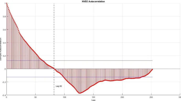
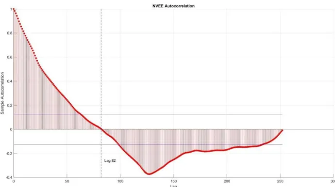
The aim of this project is to produce a short-term prediction of the price of the stock. While more data would imply a more accurate prediction, markets and stock sentiment change over time. It can thus be assumed that only a relatively small (2-8 week) window of time contains all the data relevant to a prediction. Furthermore, stocks that change drastically over time are more likely to pollute a prediction with extraneous fluctuation, especially in the short term. We must therefore extract the data relevant to a 2-3 week forecast of the market. Since we are considering the price of the stock as a stochastic process, we can use an autocorrelation to find the period of data relevant to our prediction. MATLAB has functionality to plot the autocorrelation function (ACF), defined as
for .
rk = ck
c0 k = 0 , 1, 2, ... k
c0 is the sample variance and ck is defined as
(y )(y )
ck = 1
T ∑
T−k
t=1 t−y t+k−y
where ytis a stochastic process. In the context of the autocorrelation, k is referred to as the “lag,”
or the current offset applied to the data. Essentially, the autocorrelation calculates the correlation between a time series and a delayed version of the time series for a number of lags. By
computing this function, we can extract the periods of time that show positive correlation between the past and future. In this case, we can take the window of data that exhibits positive correlation as the period of time relevant to a prediction of the future behavior of the stock, or as the period of time that contains enough data without providing too much fluctuation. We chose to define this period as the first lag at which the ACF reaches the value of 0. This ensured we captured all of the data that correlates positively before the correlation becomes unpredictable. In practice, this time period was between 2 and 8 weeks.
Figure 1: ACF Plot for NV5 Global Inc (NVEE)
Data With Trendline
After the computation of the autocorrelation, we now have a data set that can be used to predict the price of the stock. As we are considering the daily movement of the stock random, we
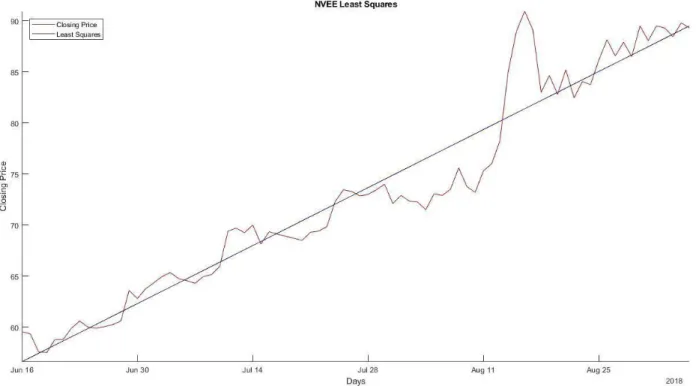
want to isolate the movement of the stock from the noise and other relevant factors. This will yield a basic prediction for the movement of the stock and allow us to estimate the random elements separately. To extract the general trend for the stock prices, we use a linear regression with the least squares method. This process assumes that individual movements are random (as in a stochastic process) and reduces the individual changes to one line that shows the general trend for the data. In the first order least squares method, an approximate function is found in the form of
.
(x) x
f = β0+ β1 i
For each data point, the residual ri is calculated using the formula .
x)
ri =yi− (β0+ β1 i
By minimizing the value of ∑m (where m is the number of data points), we can find the values
i=1ri 2
of that minimize the error between the data set and the linear fit. The resulting function thenβ provides us with the linear movement of the stock and allows us to isolate any noise. The graph below shows the trendline for one of the stocks we analyzed. This same process was repeated for all other stocks under consideration.
Figure 2: Historical Data and Trendline Plot for NVEE
Fourier Series Fit
While a linear regression gives a basic idea of how the stock price might change, this model fails to account for the random day-to-day movement that characterizes the stock market. We model this fluctuation using a Fourier series, which is defined as an approximate
representation of a function as a sum of sine and cosine functions. Mathematically, an N-term Fourier series is given by
. ⋅sin( ) 2 a0 + ∑N n=1 an 2πPnx + Φn
The more terms used, the closer the function will fit on the given interval; however, since this is a prediction, we do not want the closest possible matching only on the given interval. This is especially true given the tendency of a closely matched series to rapidly diverge to positive or negative infinity outside of the given interval. In order to prevent the series from matching to
closely and becoming wholly periodic after the given interval, we limited the number of terms based on the period of data being examined to 2, 3, or 4 terms. Longer periods afforded more terms in the Fourier series. However, using too many terms for small amount of data will
typically yield large errors in the estimation of the coefficients of the series. The data was then fit to the Fourier series using the MATLAB fit function. The fit is also done using the least squares method, using a function f(xi, )β and calculating the residuals by
. (x, )
ri =yi−f i β
By minimizing the square of the residuals, an approximation of the fluctuation is developed.
Figure 3: Fluctuation and Fourier Series for NVEE
Prediction with Error Bands
With the linear regression and the Fourier series that have analytic expressions, we can now develop a prediction. Since both of these are functions defined on a time domain, they can
be extended in to the future to form a prediction for the price of the stock. In this case, we have both the general movement of the stock (trendline) and the random day-to-day fluctuations (Fourier series). By combining the formulas for these two processes, we get a prediction for the price of the stock. However, this prediction is not inherently useful; the current prediction just provides an idea of where the stock will go and has no metric for how close the fit is or how confident the prediction is. By adding error bands, we can give a measure of confidence in our prediction and provide criteria for when real stock price diverges from predicted stock price. Error was calculated by the formula
, (x)
ri =yi−f i
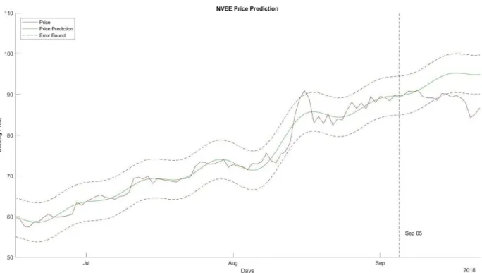
where yi is the stock data and f(xi) is the prediction. Our method of creating the error bands next required the extraction of the minimum (most negative) and maximum (most positive) error values. By taking the absolute value of these numbers and averaging them, we can create the maximum expected deviation in either direction from the prediction. This was applied as a vertical offset to the prediction and used to create two error bands on the prediction. The width of the band thus gave a confidence measurement for the price of the stock. Furthermore, when the real price of a stock leaves the error band, it can be determined to have diverged from the prediction and leaving the prediction invalid.
Figure 4: Historical Data with Prediction and Fluctuation Bands for NVEE
2) Moving Average Model
While the Fourier series can be a good predictor of large-scale fluctuations, smaller-scale fluctuations can skew the prediction and cause it to function less effectively. Some traders use moving averages to smooth the data and remove some of the daily fluctuation. The local moving average is given by . k 1 ∑k k=0 xi+k
By taking local moving averages, we can remove some extraneous fluctuation and create a more effective fit. A higher number of terms (larger k) increases the smoothing of the data. However, caution must be exercised in smoothing the data. Too much smoothing can cause the Fourier series to overfit and diverge at the end of the interval. Furthermore, the moving average moves
the data closer together in general, and can make the more significant features less intense, reducing the accuracy of the prediction.
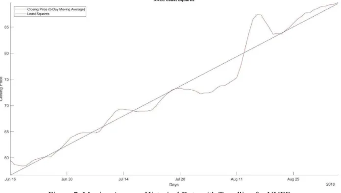
For this version of the model, a k value of 5 was used. This provided some smoothing while reducing the number of overfitting instances. k values of 3 and 10 were tested as well; 3 did not provide enough smoothing to make a difference, while 10 provided more than was necessary.
Autocorrelation
Data With Trendline
Figure 7: Moving Average Historical Data with Trendline for NVEE
Figure 8: Moving Average Fluctuation with Fourier Series for NVEE
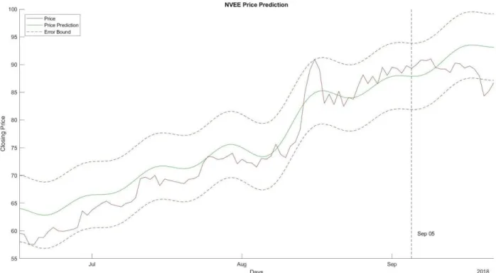
Prediction with Error Bands
Figure 9: Historical Data with Prediction and Error Bands for NVEE
3) Stock Index Cross Correlation Model
Another aspect of the stock market is indices, which consist of the prices of many different stocks. These are used to estimate performance of the market as a whole. To improve the model, we used index data to weight our predictions and increase long-term accuracy. First, in order to be able to input both data sets into the same functions, the two sets had to be normalized. We accomplished this by dividing the data sets by their present-day value (Sep 05). This moved both sets of data in to the same range. Then, a prediction was developed for both data sets (the index
and the stock price) as above. The correlation coefficient was then calculated for the two data sets. The correlation coefficient ρ(A, )B is defined as
, (A, ) ρ B = 1 N−1 ∑ N i=1
(
σA Ai−μA)(
σB Bi−μB)
where µ is the mean and σ is the standard deviation. This provides us with a value on [-1,1] that provides a measure of how well the two data sets correlate, with 1 being perfect correlation and -1 being perfect anticorrelation. To weight the stock data, we multiplied the stock prediction by , and the index prediction by and added the results together. The result was then brought
ρ 1 − ρ
back to the scale of the stock price by multiplying by the original Sep 05 value. This way, if the stock price and index correlate well, then is valued closer to 1 and more of that data is used. Ifρ the two do not correlate well, more of the index data is added in an attempt to improve the prediction. If the coefficient of correlation is negative, then it is assumed that the index does not represent the movement of the stock and is thus not useful to weight the prediction.
Figure 10: Historical Data with Prediction and Error Bands for NVEE and DJI
4) Fast Fourier Transform and Stock Index Cross Correlation
Model
The final addition to the model was the use of the Fourier transform to smooth the data and remove some of the fluctuation, in a similar manner to moving averages. The Fourier transform moves a time-valued function (our stock data) in to the frequency domain, expressing the data as the component frequencies that make it up. To find the Fourier transform, we used the Fast Fourier Transform (FFT) algorithm in MATLAB, which computes the Discrete Fourier Transform (DFT) for a set of data. The FFT and inverse FFT (IFFT) y= fft(x)and x=ifft(y) are defined as (k) (j)W Y = ∑n j=1X n (j−1)(k−1) and , (j) (k)W X = ∑n k=1Y n −(j−1)(k−1)
where Wn =e−2niπ. With the function broken in to components based on frequency, we can remove frequencies below a certain threshold to smooth the data without affecting the more significant components of frequency. This done by zeroing out any frequencies with an amplitude below a specific threshold. Similar caution had to be exercised as with moving averages to remove the correct amount of noise. Once the noise has been removed, we then use the IFFT to convert the smoothed signal back to the time domain to generate a prediction.
For the purposes of this project, a cutoff value of 10 was used. This removed a majority of the extraneous fluctuation while keeping the large, significant features intact. Smaller values tended to let too much fluctuation through, while larger values bit into the features needed to properly fit a Fourier series.
Stock FFT Prediction via Cross Correlation with Error Bands
Simulated Market Portfolio
For the last term of the project, we each built a portfolio of 10 stocks using $100,000 of virtual money to evaluate their performance across 7 weeks and potentially make a simulated profit. The stocks chosen were not solely based on model performance. To build the portfolio, we did not just rely on the model. Analyst evaluations and recommendations were consulted to create a list of stocks that would perform well in the relatively short period. Stocks that
consistently surpassed evaluations were especially favored. Stocks were then selected for low P/E and low Price/Book values. Finally, stocks that appeared to be stronger in the short term were selected over safe long-term bets to take advantage of the short timeframe.
For this stage of the project, the model was used lightly. First, the code had to be
modified, as here there is no future data to evaluate the performance of the model. Furthermore, the investing timeframe here is 7 weeks, or 49 days. This is significantly longer than even the best average predictions; therefore, the model will not be effective in predicting the behavior of the stock over the full term. Some stocks were included based on the model, however. The stocks selected based on the model were chosen due to the model’s consistent ability to predict their price.
After the portfolio was created, the closing prices of each stock was monitored
week-to-week using Yahoo Finance. Using this data, we determined whether or not each stock was making us money, as well as the overall value of the portfolio.
Results
1) Prototype Model
Symbol Days valid
Percent Bandwidth ACM 15 5.10% CAT 8 5.18% DHI 3 8.59% EME 0 3.06% FLR 16 7.55% JEC 17 7.19% KBR 0 4.01% LPX 6 6.01% MTZ 4 6.18% NVEE 11 15.93% PWR 5 4.62% STRL 1 11.37% TEX 5 9.84% UTX 9 3.79% VMC 9 2.49% HPQ 5 5.29% DBX 2 14.79% NLSN 2 28.74% T 4 6.24% TWTR 11 25.76% INTC 12 10.59% YELP 2 17.35% ORCL 2 2.72% ATVI 2 6.64% NTGR 2 11.44% TMUS 1 5.26% NTDOY 3 6.14% KNMCY 0 8.83% SNE 6 4.72% TCTZF 1 11.11%
Average 5.47 8.88%
Stdev 4.94615 6.29%
The original model without any additions managed to predict the price of a stock for 5.47 days on average before diverging. However, this data is characterized by a very large standard deviation of 4.95 days. This is due to most stocks either performing very well or very poorly, causing it to be pulled in both directions by near perfect and completely ineffectual predictions. The error was decent at 8.88% ± 6.29%, meaning the error was in almost all cases below 15% of the price of the stock. While not ideal, it is enough to predict the stock price in the very short term.
2) Moving Average Model
Symbol Days valid
Percent Bandwidth ACM 13 2.25% CAT 4 1.81% DHI 1 3.47% EME 0 2.02% FLR 8 5.30% JEC 14 4.43% KBR 0 2.74% LPX 6 2.15% MTZ 3 2.24% NVEE 7 8.68% PWR 5 3.07% STRL 1 6.89% TEX 2 2.82% UTX 5 0.93% VMC 2 0.79% HPQ 5 2.11% DBX 0 8.43% NLSN 0 13.14%
T 0 3.05% TWTR 7 15.87% INTC 1 5.42% YELP 0 6.29% ORCL 2 1.38% ATVI 1 4.14% NTGR 0 4.52% TMUS 0 1.68% NTDOY 0 2.32% KNMCY 0 5.50% SNE 6 2.54% TCTZF 0 4.90% Average 3.10 4.36% Stdev 3.83586 3.46%
Adding moving averages to smooth the data actually made the prediction much worse, averaging only 3.10 days with a comparatively massive 3.84 standard deviation. This is most likely due to oversmoothing or too strong of a fit to the data by the Fourier series. This is evidenced by the much smaller error bandwidth, which is nearly half of that of the original model.
3) Stock Index Cross Correlation Model
Adjusted Days valid Adjusted Percent Bandwidth
DJI GSPC IXIC RUT DJI GSPC IXIC RUT
ACM 17 17 17 17 8.41% 10.42% 10.44% 8.57% CAT 0 9 9 5 0.00% 7.16% 8.80% 9.43% DHI 2 2 2 2 9.06% 8.90% 10.10% 9.57% EME 1 2 2 0 3.22% 3.31% 3.94% 0.00% FLR 17 17 17 17 7.89% 7.82% 7.74% 9.14% JEC 17 17 17 0 7.18% 7.20% 7.13% 0.00% KBR 1 1 1 0 4.07% 4.13% 4.95% 0.00% LPX 0 8 9 8 0.00% 8.48% 8.98% 7.51%
MTZ 0 0 0 10 0.00% 0.00% 0.00% 12.91% NVEE 14 14 14 14 17.17% 16.12% 14.29% 16.21% PWR 5 7 0 0 7.30% 8.60% 0.00% 0.00% STRL 4 4 5 6 12.75% 12.51% 12.76% 13.29% TEX 0 0 0 0 0.00% 0.00% 0.00% 0.00% UTX 9 9 9 0 4.08% 4.19% 5.28% 0.00% VMC 0 6 6 0 0.00% 3.70% 3.52% 0.00% HPQ 8 6 5 5 6.33% 5.77% 5.42% 5.44% DBX 0 0 17 0 0.00% 0.00% 22.45% 0.00% NLSN 0 0 0 0 0.00% 0.00% 0.00% 0.00% T 0 0 0 0 0.00% 0.00% 0.00% 0.00% TWTR 0 0 17 17 0.00% 0.00% 45.58% 39.50% INTC 0 0 0 0 0.00% 0.00% 0.00% 0.00% YELP 2 2 0 2 18.55% 19.43% 0.00% 18.23% ORCL 2 10 0 7 4.14% 4.69% 0.00% 6.87% ATVI 3 3 3 3 18.75% 15.23% 13.29% 11.96% NTGR 11 11 17 11 16.94% 15.55% 15.40% 13.88% TMUS 1 1 1 1 5.71% 5.71% 6.09% 6.08% NTDOY 3 3 4 3 6.34% 6.45% 6.89% 6.63% KNMCY 0 0 0 0 0.00% 0.00% 0.00% 0.00% SNE 6 6 6 6 4.94% 4.85% 4.96% 5.42% TCTZF 0 0 0 0 0.00% 0.00% 0.00% 0.00% Avg 6.83333 7.38095 8.9 7.8823 9.05% 8.58% 10.90% 11.80% Stdev 5.93345 5.34300 6.26519 5.53266 5.34% 4.64% 9.42% 8.09%
A number of different indices were used for this version of the model. As such,
successful predictions and average days were computed slightly differently. If the coefficient of correlation came out negative for a given prediction, that prediction was considered to have failed for that index and the data for that stock was not counted. Most stocks had a successful correlation with at least one index, the exceptions being TEX, NLSN, T, INTC, KNMCY, and TCTZF. For performance, all improved on the base model drastically. The best performing index was the S&P 500 (GSPC), which despite 11 failed predictions added 1.9 days to its average over the base model, while keeping a similar standard deviation. Additionally, both the average error
bandwidth and its standard deviation decreased. Overall, despite the couple of failed predictions, the index weighted method performs significantly better than the base model.
4) Fast Fourier Transform and Stock Index Cross Correlation
Model
Adjusted Days valid Adjusted Percent Bandwidth
DJI GSPC IXIC RUT DJI GSPC IXIC RUT
ACM 17 17 17 17 8.05% 8.92% 8.95% 8.16% CAT 0 9 8 5 0.00% 8.02% 9.26% 9.49% DHI 10 10 12 12 10.59% 10.42% 11.44% 11.16% EME 0 0 0 3 0.00% 0.00% 0.00% 3.79% FLR 0 0 0 0 0.00% 0.00% 0.00% 0.00% JEC 0 0 0 1 0.00% 0.00% 0.00% 7.67% KBR 4 4 5 0 6.74% 6.78% 6.97% 0.00% LPX 0 10 10 8 0.00% 10.96% 11.25% 10.43% MTZ 0 0 0 12 0.00% 0.00% 0.00% 15.82% NVEE 15 14 14 15 18.69% 16.53% 16.45% 17.44% PWR 0 0 14 13 0.00% 0.00% 12.56% 10.17% STRL 13 14 14 14 15.90% 15.90% 15.72% 15.91% TEX 0 0 0 0 0.00% 0.00% 0.00% 0.00% UTX 9 9 7 0 4.52% 4.65% 5.84% 0.00% VMC 0 9 6 0 0.00% 4.22% 4.12% 0.00% HPQ 1 1 1 0 2.85% 2.20% 2.25% 2.31% DBX 0 0 0 0 6.64% 6.69% 6.91% 6.67% NLSN 0 0 0 0 0.00% 0.00% 0.00% 0.00% T 0 0 0 0 0.00% 0.00% 0.00% 0.00% TWTR 0 0 17 17 0.00% 0.00% 40.96% 34.22% INTC 0 0 0 0 0.00% 0.00% 0.00% 0.00% YELP 5 7 0 5 11.15% 11.74% 0.00% 10.84% ORCL 0 0 0 0 0.00% 0.00% 0.00% 0.00% ATVI 3 3 3 3 16.28% 12.94% 10.86% 9.57% NTGR 10 11 17 11 15.62% 14.34% 13.96% 12.79% TMUS 1 1 1 1 3.69% 3.49% 3.48% 3.46% NTDOY 3 3 3 2 4.18% 3.84% 3.69% 3.58% KNMCY 0 0 0 0 0.00% 0.00% 0.00% 0.00%
SNE 6 6 6 6 6.28% 6.92% 6.68% 6.44%
TCTZF 0 0 0 0 0.00% 0.00% 0.00% 0.00%
Avg 6.92857 7.52941 8.61111 8.05556 9.37% 8.74% 10.63% 10.52%
Stdev 5.4697 5.01396 5.91249 5.85584 5.35% 4.48% 8.67% 7.19%
The usage of the Fourier transform to filter the data had a similar improvement over the weighted model. Despite more failed predictions, the altered model managed to slightly extend its averages while decreasing the standard deviations and overall error bandwidths. In this case, FLR, TEX, NLSN, T, INTC, ORCL, KNMCY, and TCTZF failed to be predicted by the model, while JEC and EME could only be predicted (quite poorly) by RUT. Therefore, while this model is the most effective, there is a chance it is unable to accurately predict a stock at all, and will require additional analysis to determine if its application is appropriate. While it can be assumed that a stock listed on specific index will be predicted by that index, this is not the case; many stocks are predicted well by indices that they are not listed on, and vice versa. Instead, a more basic assumption that the behavior of some stocks is not reflected by all indices is more likely, and is reinforced by cases such as FLR.
Virtual Portfolio 1
1/14-1/21
Stock Change Percent Change Profit/Loss AMD $0.50 2.47% $246.67 CMI $11.02 7.90% $789.74 DHI -$2.42 -6.11% -$611.11 GE $0.12 1.34% $134.23 NUE $2.14 3.78% $378.16 NVEE $2.13 3.18% $318.24 PFE -$0.35 -0.82% -$81.62 SNDR $1.12 5.52% $552.27
STRL $0.80 6.40% $640.00 UTX $3.95 3.59% $359.25 Weekly Net $2,725.83 2.73%
The first week showed strong gains from CMI, SNDR, and STRL. DHI drops in value significantly, however, is the only stock to do so. This week results in a 2.73% profit, or $2,725.83.
1/21-1/28
Stock Change Percent Change Profit/Loss AMD $1.16 5.58% $572.27 CMI -$3.72 -2.47% -$266.59 DHI $0.12 0.32% $30.30 GE $0.10 1.10% $111.86 NUE -$0.63 -1.07% -$111.33 NVEE $1.33 1.93% $198.72 PFE -$1.89 -4.44% -$440.76 SNDR -$0.34 -1.59% -$167.65 STRL $0.18 1.35% $144.00 UTX $4.17 3.66% $379.26 Weekly Net $450.08 0.45%
This week had significantly more losses, but none as severe as the week prior. AMD performed well, while PFE performed the worst by far. This week resulted is a 0.45% profit, or $450.08.
1/28-2/4
Stock Change Percent Change
Profit/Loss
CMI -$0.13 -0.09% -$9.32 DHI $0.69 1.85% $174.24 GE $1.03 11.24% $1,152.13 NUE $3.38 5.82% $597.28 NVEE $1.66 2.36% $248.02 PFE $2.24 5.51% $522.39 SNDR $0.73 3.47% $359.96 STRL -$0.30 -2.23% -$240.00 UTX $0.91 0.77% $82.76 Weekly Net $4,160.28 4.16%
This week, AMD and GE shot up with a combined change of 23%. In addition, the only losses were small, resulting in a 4.16% profit, or $4,160.28.
2/4-2/11
Stock Change Percent Change Profit/Loss AMD -$1.46 -6.33% -$720.28 CMI $1.57 1.06% $112.51 DHI -$0.27 -0.72% -$68.18 GE -$0.76 -8.06% -$850.11 NUE -$1.66 -2.77% -$293.34 NVEE $1.18 1.61% $176.30 PFE $0.14 0.33% $32.65 SNDR -$0.05 -0.23% -$24.65 STRL -$0.09 -0.69% -$72.00 UTX $3.51 2.87% $319.24 Weekly Net -$1,387.86 -1.39%
This week contained the only loss. After huge gains the previous week, AMD and GE both dropped in value. This decrease, however, was smaller than the previous week’s increase, leaving a net positive over the two weeks. Most other stocks stayed the same or dropped in
value, except for UTX, which continues its steady climb. This week resulted in a 1.39% loss, or -$1387.86.
2/11-2/18
Stock Change Percent Change Profit/Loss AMD $0.08 0.35% $39.47 CMI $3.11 2.05% $222.88 DHI $2.08 5.23% $525.25 GE $0.22 2.28% $246.09 NUE -$0.09 -0.15% -$15.90 NVEE $2.86 3.76% $427.31 PFE -$1.05 -2.50% -$244.87 SNDR $1.52 6.53% $749.51 STRL $0.47 3.47% $376.00 UTX $1.64 1.32% $149.16 Weekly Net $2,474.88 2.47%
This week saw most stocks rebound from drops last week. SNDR showed particularly strong growth at 6.53%. This week resulted in a profit of 2.47% or $2,474.88, larger than last week’s loss.
2/18-2/25
Stock Change Percent Change Profit/Loss AMD $1.23 5.05% $606.81 CMI $4.05 2.61% $290.24 DHI $1.04 2.55% $262.63 GE $0.13 1.33% $145.41 NUE $1.46 2.39% $258.00 NVEE $4.34 5.40% $648.44 PFE $0.99 2.30% $230.88 SNDR -$0.28 -1.22% -$138.07 STRL $1.15 7.82% $920.00
UTX $3.64 2.85% $331.06 Weekly Net $3,555.39 3.56% Gross Net $11,978.60 11.98%
The last week saw further gains across the board, with STRL performing exceptionally well with a 7.82% increase. This week resulted in a gain of 3.56%, or 3,555.39. Overall, the portfolio increased in value by 11.98% over the 7 weeks, for a total gain of $11.978.60.
Overall
Stock Change Percent Change Profit/Loss AMD $4.09 20.18% $2,017.76 CMI $15.90 11.39% $1,139.46 DHI $1.24 3.13% $313.13 GE $0.84 9.40% $939.60 NUE $4.60 8.13% $812.86 NVEE $13.50 20.17% $2,017.03 PFE $0.08 0.19% $18.66 SNDR $2.70 13.31% $1,331.36 STRL $2.21 17.68% $1,768.00 UTX $17.82 16.21% $1,620.74 Average 11.98% $1,197.86 Stdev 6.88% $687.72
Over the 7 weeks, the average increase of each stock was 11.98%, with a standard deviation of 6.88%, resulting in an average profit of $1,197.86 per stock with a standard
deviation of $687.72. It should be noted that while the smallest gains were quite low (0.19% for PFE), no stocks actually lost money overall.
Virtual Portfolio 2
1/14-1/21
Stock Change Percent Change Profit/Loss AMD $0.50 2.47% $250.00 CSCO $1.54 3.54% $885.00 EA $1.82 2.01% $182.00 HPQ $0.58 2.74% $290.00 INTC $0.26 0.53% $52.00 MDB $5.86 7.87% $879.00 MLNX -$2.66 -3.10% -$266.00 ORCL $0.98 2.03% $196.00 SNE $1.20 2.45% $240.00 SQNXF $0.90 3.00% $270.00 Weekly Net $2,978.00 2.98%
The first week resulted in most stocks making around $200, which is quite satisfactory. MLNX was the only stock to drop in value, but the large increase in CSCO and MDB’s stocks more than made up for it. Overall, the first week produced a profit of $2,978.00, or 2.98% of the original cost.
1/21-1/28
Stock Change Percent Change Profit/Loss AMD $1.16. 5.59% $580.00 CSCO $1.10 2.44% $275.00 EA -$0.78 -0.84% -$78.00 HPQ $0.75 1.61% $375.00 INTC -$2.15 -4.37% -$430.00 MDB $6.56 8.17% $984.00 MLNX $2.30 2.77% $230.00 ORCL $0.53 1.08% $106.00
SNE -$1.42 -2.83% -$284.00 SQNXF $1.21 3.91% $363.00 Weekly Net $2,121.00 2.12%
During the second week, MDB continued to provide excellent results. The stocks that previously decreased have now begun to produce a profit instead. However, in their stead, EA, INTC, and SNE are now resulting in a loss. The week resulted in a profit of $2,121.00, or 2.12% of the original cost.
1/28-2/4
Stock Change Percent Change Profit/Loss AMD $2.58 11.77% $1,290.00 CSCO $1.21 2.62% $302.50 EA -$0.52 -0.57% -$52.00 HPQ $0.16 0.72% $80.00 INTC $1.69 3.59% $338.00 MDB $5.77 6.64% $865.50 MLNX $10.28 12.05% $1,028.00 ORCL $1.01 2.03% $202.00 SNE -$2.61 -5.35% -$522.00 SQNXF $0.75 2.33% $225.00 Weekly Net $3,757.00 3.76%
The third week ended up producing the greatest results of all, with AMD and MLNX creating staggering profits of over $1,000.00 each. Additionally, INTC was once again producing a profit. The overall result was a 3.76% profit, equivalent to $3,757.00.
2/4-2/11
Stock Change Percent Change Profit/Loss AMD -$1.46 -5.96% -$730.00 CSCO -$0.15 -0.32% -$37.50 EA $6.38 6.99% $638.00 HPQ $0.66 2.97% $330.00 INTC $0.11 0.23% $22.00 MDB $5.68 6.13% $852.00 MLNX $1.54 1.61% $154.00 ORCL $0.22 0.43% $44.00 SNE -$1.86 -4.03% -$372.00 SQNXF -$3.96 -12.04% -$1,188.00 Weekly Net -$287.50 -0.29%
The fourth week ended up being the only week to result in an overall loss. Despite this, MDB continued to produce a large profit. As a result, the week ended with $287.50 being lost. Fortunately, this was only 0.29% of the original cost.
2/11-2/18
Stock Change Percent Change Profit/Loss AMD $0.08 0.35% $40.00 CSCO $1.21 2.56% $302.50 EA $7.65 7.84% $765.00 HPQ $0.31 1.35% $155.00 INTC $1.97 4.03% $394.00 MDB $0.94 0.96% $141.00 MLNX $3.30 3.40% $330.00 ORCL $0.45 0.88% $90.00 SNE $0.83 1.87% $166.00 SQNXF $1.63 5.64% $489.00 Weekly Net $2,872.50 2.88%
The fifth week was the only week where all stocks ended up creating a profit, albeit not that much. Still, this resulted in the decent gain of $2872.50, or 2.88%.
2/18-2/25
Stock Change Percent Change Profit/Loss AMD $1.23 5.32% $615.00 CSCO $1.71 3.53% $427.50 EA -$9.33 -8.87% -$933.00 HPQ $0.51 2.20% $255.00 INTC $1.68 3.31% $336.00 MDB $6.92 6.97% $1,038.00 MLNX $4.53 4.51% $453.00 ORCL $1.00 1.94% $200.00 SNE $2.77 6.14% $554.00 SQNXF -$1.55 -5.07% -$465.00 Weekly Net $2,480.50 2.48% Gross Net $13,921.50 13.94%
The final week resulted in a typical profit of $2480.50. Once again, EA and SQNXF went down in price, while MDB sore upwards. This all meant a 2.48% increase. Thus, by the end of the 7 weeks, the portfolio produced a total gain of $13,921.50, or 13.94% of the stocks’ original costs of $99,855.
Overall
Stock Change Percent Change
Profit/Loss AMD $4.09 20.18% $2,045.00
CSCO $6.62 15.22% $1,655.00 EA $5.22 5.76% $522.00 HPQ $2.57 12.14% $1,285.00 INTC $3.56 7.28% $712.00 MDB $31.73 42.60% $4,759.50 MLNX $19.29 22.51% $1,929.00 ORCL $4.19 8.68% $838.00 SNE -$1.09 -2.23% -$218.00 SQNXF -$1.02 -3.40% -$306.00 Average 12.88% $1,322.15 Stdev 13.45% $1,456.33
After the period of 7 weeks, the investments proved to be a success, with an average of 12.88% increase in stock value. This was equivalent to each stock growing by $1322.15. However, the standard deviations were also relatively large, portraying the fact that SNE and SQNXF actually went down in value. On the other hand, the large standard deviations were also a result of some of the stocks making comparatively substantial increases, such as AMD, MDB, and MLNX.
Summary
Based on the data, the best-performing iteration of the model was the version that used indices to weight the prediction and used the FFT algorithm to filter the data. While this iteration gave very polarized performance (either predicting the stock very well or failing to predict at all), the model was able to predict the price of a stock for at least 10 days on average, depending on the index used. However, this version of the model did suffer from a larger error of 10% on average. Despite this, on average it predicts the price of a stock for 1-3 days longer than the weighted model without filtering using the FFT. The improvement over the prototype model is
even larger, increasing the average error by 4% in exchange for lengthening the prediction by 3-4 days.
For the virtual portfolio, the endeavor was quite successful, with the first netting an 11.98% profit over 7 weeks, and the second a 12.88% profit. While the methods used were inexact as best, a similar strategy can be used to make money in the short term using the stock market. Stocks were not evaluated after the portfolio period to determine how well the model would have performed.
Recommendations
MATLAB has a large library of functions for filtering data. Given the positive
performance of using the FFT algorithm to remove noise, other methods of filtering noise from the stock data could be explored. Additionally, the amount of volatility a stock historically experienced could be viewed as a forewarning of its unpredictability in the future. By examining the volume of a stock and ascertaining a correlation with its volatility, it could be possible to detect how reliable or consistent a prediction of that stock might be, just from its volume.
Bibliography
MathWorks. “MATLAB Documentation,” R2018b. MathWorks Documentation. MathWorks, 2018, https://www.mathworks.com/help/matlab/. Accessed 9/12/2018.
Haddad, Spenser Adam, et al. Trading System Development: Trading a System of Systems . 2013,
Trading System Development: Trading a System of Systems ,
web.wpi.edu/Pubs/E-project/Available/E-project-042313-234712/unrestricted/System_of_Syste
“Relative Strength Index (RSI).” How Mutual Funds, ETFs, and Stocks Trade - Fidelity,
www.fidelity.com/learning-center/trading-investing/technical-analysis/technical-indicator-guide/
rsi.
Huey, Burkett. “Our Ultimate Stock-Pickers' Top 10 Buys and Sells.” Morningstar.com, 5 Sept. 2018,
www.morningstar.com/articles/881740/our-ultimate-stockpickers-top-10-buys-and-sells.html.
Stephen, Gandel. “Stocks Face Obstacle No Matter What the Fed Does.” Bloomberg.com, Bloomberg, 19 Dec. 2018, 7:00 AM EST,
www.bloomberg.com/opinion/articles/2018-12-19/stocks-face-obstacle-no-matter-what-the-fed-does.
Kenton, Will. “Autocorrelation.” Investopedia, Investopedia, 5 July 2018,
www.investopedia.com/terms/a/autocorrelation.asp.
Kalid. “An Interactive Guide To The Fourier Transform.” BetterExplained, BetterExplained, 2013, betterexplained.com/articles/an-interactive-guide-to-the-fourier-transform/.
Hadley, Erin A. “How to Build a Stock Portfolio.” WikiHow, WikiHow, 12 Feb. 2019,
www.wikihow.com/Build-a-Stock-Portfolio.
Hoy, Laura. “Is AMD Stock Really a Best Bet for 2019?” Yahoo! Finance, InvestorPlace, 18 Dec. 2018, 10:33 am EST, finance.yahoo.com/news/amd-stock-really-best-bet-153332593.html. Duberstein, Billy. “MongoDB Continues to Impress.” Yahoo! Finance, The Motley Fool, 24 Dec. 2018, finance.yahoo.com/news/mongodb-continues-impress-173000959.html.
Stock data taken from finance.yahoo.com Graphs generated using MATLAB