An eddy-resolving Reynolds stress model for
unsteady flow computations: development and
application
Vom Fachbereich Maschinenbau an der Technischen Universität Darmstadt
zur
Erlangung des Grades eines Doktor-Ingenieurs (Dr.-Ing.) genehmigte
D i s s e r t a t i o n
vorgelegt von
Dipl.-Ing. Robert Maduta
aus Bukarest
Berichterstatter: Prof. Dr.-Ing. C. Tropea Mitberichterstatter: Apl. Prof. Dr.-Ing. S. Jakirlic
Apl. Prof. Dr. rer. nat. A. Sadiki Tag der Einreichung: 04.02.2013
Tag der mündlichen Prüfung: 29.05.2013 Darmstadt 2013 D17 (Diss. Darmstadt)
Hiermit versichere ich, die vorliegende Doktorarbeit unter der Betreuung von Prof. Dr.-Ing. C. Tropea nur mit den angegebenen Hilfsmitteln selbständig angefertigt zu haben.
Abstract
The present study focuses on a turbulence modeling strategy aiming at advancement of the Reynolds-averaged Navier-Stokes (RANS) approach. The modeling strategy relies on an anisotropy-resolving near-wall second-moment closure model, which is extended to behave as an eddy-resolving model with respect to capturing spatial and temporal variability of turbu-lence scales. The model should not comprise any parameter depending ex-plicitly on the grid spacing. It means the objective is to formulate a “true” Unsteady RANS (URANS) model. An additional term in the correspond-ing length-scale determincorrespond-ing equation providcorrespond-ing a selective assessment of its production represents a key parameter in this novel URANS approach. This term modeled in terms of the von Karman length scale representing the ratio of the second to the first derivative of the velocity field in line with the scale-adaptivity concept (SAS - scale adaptive simulation) introduced
by Menter and Egorov [35]. In addition, the background RANS model
has been “numerically stabilized” by reformulating some terms - primarily diffusive transport and gradient production - in conjunction with an appro-priately defined wall boundary condition for the dissipation rate of kinetic energy of turbulence. Herewith, the use of high-order numerical schemes,
such as 2ndorder central differencing scheme, is promoted; this issue is of
crucial importance with respect to preventing the possible fallback from mainly resolved turbulent structures to modeled ones.
The predictive performances of this instability-sensitive, eddy-resolving model was checked by computing different flow cases including separation from a sharp-edged surface (backward-facing step configurations) and con-tinuous flat and curved surfaces (flow past a tandem cylinder configuration, flow over a 2D Hill and in a 3D Diffuser in a range of geometrical parame-ters and Reynolds numbers). The results obtained are in closest agreement with available reference data, outperforming significantly the results perti-nent to the conventional model of turbulence. Prior to that several globally stable flows, such as natural decay of homogeneous isotropic turbulence and flow in a plane channel have been computed in course of the model calibra-tion. It should be emphasized that in all cases considered the fluctuating
Finally, an appropriate modification of the background second-moment closure model in the “Steady RANS” framework is proposed leading to substantially improved turbulence level prediction - and consequently the mean flow field - in the separating flow regions; by simultaneously retaining good results in attached flow regions.
Kurzfassung
Die vorliegende Doktorarbeit befasst sich mit der Entwicklung und Anwen-dung eines neuartigen, instationären Reynolds-gemittelten Navier-Stokes (URANS) Modells, welches als Basis das Skalen-adaptive Konzept (SAS),
eingeführt von Menter und Egorov [35], verwendet. Durch Kombination
mit einem Reynolds Spannungs Modell, welches den statistischen Ansatz wiedergibt, ist das neue Modell in der Lage, wie man im Laufe dieser Ar-beit sehen wird, turbulente Strukturen in der Strömung aufzulösen ohne in einer Gleichung die explizite Gitterabhängigkeit zu benötigen. Der Schlüs-selparameter ist dabei ein zusätzlicher Term in der Dissipationsgleichung, welcher selektiv die Produktion der Dissipation in angemessener Weise er-höht. Er besteht aus dem Verhältnis der zweiten zur ersten Ableitung des Geschwindigkeitsfeldes. Die Stabilisierung des Reynolds Spannungs Modells in numerischer Hinsicht, durch die Umformulierung bestimmter Terme und das Abändern einer Wandrandbedingung, ist unerlässlich um numerische Diskretisierungsschemata hoher Ordnung verwenden zu kön-nen, welche einen Wechsel von hauptsächlich aufgelösten, turbulenten Struk-turen zu Modellierten vermeiden.
Es werden im Zuge dieser Arbeit verschiedene Anwendungsfälle mit Strö-mungsablösungen von gekrümmten Oberflächen (Anordnung von zweidi-mensionalen Hügeln, der dreidimensionale Diffusor sowie eine Tandemzylin-deranordnung), von spitzen Kanten (zurückspringende Stufe) sowie auch Solche ohne Ablösungen (ebener Kanal, Zerfall von turbulenten Struk-turen ohne äußere Einwirkung) berechnet werden. Des weiteren werden die durchweg positiven Ergebnisse mit Referenzdaten verglichen werden um die quantitative Effizienz des neuartigen Modells offenzulegen. Es gilt an dieser Stele festzuhalten, dass in allen berechneten Fällen das Modell von sich aus in einen Strukturauflösenden Modus gewechselt ist, wobei jede Simulation auf ein stationäres Feld gestartet wurde.
In dem letzten Abschnitt befasst sich diese Arbeit mit einer Modifikation des Reynolds Spannungs Modells innerhalb der stationären Simulations-möglichkeiten. Es wird gezeigt werden, dass mit einer leichten Abänderung
Strömungen erzielt werden können, ohne jedoch die gute Berechenbarkeit von angelegten Strömungen zu beeinflussen.
Acknowledgements
Financial support by the European project ATAAC is gratefully acknowl-edged.
This work has been carried out at the Institute of Fluid Dynamics and Aerodynamcs SLA of the Technische Universität Darmstadt during the pe-riod between April 2009 to September 2012.
I would like to thank Prof. Dr.-Ing. habil. Cameron Tropea and Apl. Prof. Dr.-Ing. habil. Suad Jakirlic for the possibility to do this work and for their helpful comments on the present work. Especially Apl. Prof. Dr.-Ing. habil. Suad Jakirlic very often helped me out with his deep knowledge in turbulence modeling. He always took his time answering my questions, while he guided me in the right direction if necessary. I would also like to thank my family and my girlfriend Christina who supported and encour-aged me, especially during the last months. My cousin Anamaria was a great help with correcting a lot of my English grammar.
Finally I would like to thank my colleagues from the SLA Institute for creating a pleasant atmosphere and the secretaries for handling all the ad-ministrative issues.
Contents
Abstract i Kurzfassung iii Acknowledgements v 1 Introduction 1 1.1 Motivation . . . 1 2 Theoretical Background 52.1 Basics of the finite volume-based numerical method. . . 5
2.2 Turbulence modeling . . . 9
3 Derivation of an eddy-resolving Reynolds stress model (RSM) 15
3.1 Transformation fromǫh toωh . . . . 15
3.2 Full model calculations withωh based JH-RSM . . . . 18
3.2.1 Turbulent channel flow. . . 22
3.3 From Rotta’skL equation to the instability sensitive model 26
4 Testcase results 35
4.1 Decay of homogeneous isotropic turbulence . . . 35
4.2 Turbulent channel flow atReτ = 395 . . . 38
4.3 Turbulent Flow over a 2D Hill with different Reynolds numbers 43
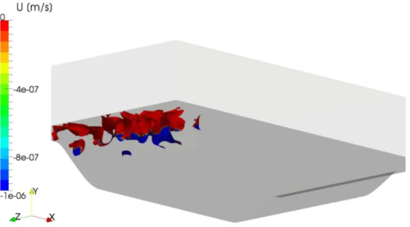
4.4 Turbulent flow in a 3D Diffuser . . . 52
4.5 Flow over a backward-facing step . . . 61
4.6 Turbulent flow past a tandem cylinder configuration . . . . 66
4.6.1 Large distance caseL/D= 3.7 . . . 69
4.6.2 Short distance caseL/D= 1.435 . . . 73
4.6.3 Root mean square of surface pressure distribution . 76
5 A RANS RSM model accounting for selective turbulence
produc-tion enhancement 81
5.1 Testcase results with the JH-RSM(−PSAS) . . . 88
5.1.2 Turbulent mixing layer. . . 90
5.1.3 Flow over a backward-facing step . . . 93
5.1.4 Turbulent flow over a 2D Hill . . . 95
5.1.5 Turbulent flow in a 3D Diffuser . . . 99
6 Conclusions and Outlook 103
Bibliography 107 Nomenclature 113 List of Figures 119 List of Tables 121 Appendix A 123 Appendix B 125
1 Introduction
1.1 Motivation
Turbulence in connection with fluid flow occurs in a great variety of oc-casions with industrial relevance but also in every day situations. Exter-nal aerodynamics (flow over wings or plane bodies), interExter-nal aerodynamics (flow through compressor and turbine configurations), external and inter-nal hydrodynamics (ship and pipe flows), combustion and weatherforecast just to mention a few. Since it obviously plays an important role, the
understanding of the phenomenon is promoted for a fairly long time [46].
Nowadays, with increasing computer power, computational fluid dynam-ics (CFD) have developed as a principal supporter for experimental work. The equations governing the particular turbulent flow problem, are solved numerically on a modeled grid reflecting the actual geometry of interest. To not only support, but also substitute experiments, the results of the computer simulations have to be quite accurate and fast. The two points are in contradiction to each other as will be shown in the following. The most accurate way to compute a turbulent flow numerically, is by directly solving the transport equations for momentum, energy and the continuity equation, which is called direct numerical simulation (DNS). By directly solving, it is meant that no mathematical model describing and simplifying physics in conjunction with turbulence is used. It is by defi-nition accurate, but it also implies that every effect has to be resolved, in the sense that the numerical grid as well as the chosen time step inside the computation have to be fine enough not to lose any kind of information. Since no model is used, lost information is fed immediately into the trans-port equations leading consequently to wrong predictions of the flow field. An important parameter which describes, on a certain level, how
turbu-lent a flow problem really is, is the so called Reynolds number Re. The
Reynolds number, which is basically the ratio between inertia and viscous
forces, can be expressed by a characteristic velocity U, a characteristic
length scale H and the molecular viscosity ν with Re =U H/ν.
increase in turbulent structures and a decrease in structure sizes at the smaller levels. The number of points needed for the numerical grid scales
approximately withRe3 for a DNS [43]. This is a very steep increase and
limits automatically the use of this method to very abstract and simple ge-ometries with very low Reynolds numbers. Even with, the nowadays highly increasing computer power, a DNS won’t be feasible for industrial relevant cases for many decades. One further problem is the fact, that many parts of the coupled differential equations are solved implicitly, which leads to a disproportionate increase of computational time needed, with increasing the number of gridpoints. To overcome this problem, turbulence models have been introduced in the early 70’s starting with the work of Hanjalic,
Spalding and Launder [16] [31]. They made use of the average procedure
on the differential equations introduced by Reynolds [47]. With that, the
turbulent flow problem is described in its average, with the equations con-taining an extra term that describes the turbulent interaction and has to be modeled. Due to the averaging procedure such kind of models are known as Reynolds Averaged Navier-Stokes models. Since the turbulent interactions as a whole are modeled, relatively coarse computational grids can be used. If one homogeneous direction exists in the flow field (homogeneous in terms of averaged quantities) the complete third dimension can be skipped, since the impact coming from the third dimension is anyhow accounted for by the model. Very large time steps can be used since again only the average of the flow quantities is computed.
The extra term in the averaged momentum equation, called Reynolds stress tensor, can be described by different approaches, of which the second mo-ment closure is the most sophisticated one. It prescribes for each quantity inside the symmetric tensor a differential equation leading to six coupled differential equations. RANS models can give for a variety of turbulent flow cases very accurate results. With fine tuning of model constants, even for complicated cases reasonable results can be obtained. In industrial ap-plications one has to compute more or less very similar topologies. Once problems have been detected with RANS models for particular cases they
can be ad hoc modified for special interest. Which is a quick and very
efficient procedure but suffers from reasonable physical background. Nevertheless there are typical turbulent flows where RANS models fail sub-stantially. One of these is the massively separated flow from curved sur-faces, which is a typical situation in external and internal aerodynamics where the flow separates from from plane wings at high angle of attack of from compressor blades at the leading edge. The so called large eddy
simu-1.1 Motivation
lation (LES) tries to bridge the gap between DNS and RANS by modeling the small turbulent structures and resolving the large ones. This is done by filtering the transport equations, which seems at first to be an adequate procedure, but has been shown to be too costly for higher Reynolds number
engineering applications [43] in terms of computational effort; hence this
approach remains unfeasible except for some very basic turbulent flow cases. The motivation of the present work is to develop a turbulence model which, on the one hand is accurate enough for massively separated flows, and on the other hand is closer to RANS than to DNS in terms of required com-putational resources. The approach taken to achieve these goals was to
introduce the scale adaptive simulation concept [35] into a second moment
closure RANS model. By doing so the RANS model can be triggered to re-solve turbulent flow structures without the explicit use of grid parameters, but rather by using the ratio between first and second velocity derivatives. It will be shown that the new model can be used with much coarser grids than LES demands, due to the continuous and variable shift between the resolved and the modeled part. In fact often the same grid can be used as the RANS simulation would need but extended in a relatively coarse manner in third dimension. Since turbulent structures are resolved, the simulation with this new model must be carried out time dependent. As the grid is much coarser than for LES or DNS, also larger timesteps can be used. It will be shown that by coupling the SAS concept with a sec-ond moment closure model, also called Reynolds stress model (RSTM or RSM), and implementing slight modifications and calibration, this newly developed model is able to switch also under quasi stable flow conditions without separations, like for example the turbulent flow in a plane channel, in a structure resolving mode. This distinguishes its features from the SAS
concept introduced by Menter and Egorov [35].
The final part of this work addresses a modified RANS model which is able to handle massively separated flows by performing steady state
simu-lations, often on two-dimensional grids. The modifications are notad hoc
and the derivation together with the underlying idea will be presented. It consists of a different approach in deriving a length-scale supplying equa-tion and basically makes use of the term introduced in the SAS concept but with an opposite sign. It will be shown that with this RANS model important turbulent flow cases which are known to be well computed by the baseline RANS model, are not influenced by the proposed modifications.
2 Theoretical Background
The computations for this dissertation have been done with OpenFOAM
[41], an open source finite volume program package. First a short
descrip-tion of the finite volume method is given, accompanied by the presentadescrip-tion
of the Jakirlic-Hanjalic Reynolds stress model (JH-RSM [19]). The latter
is the starting point for the turbulence modeling that is going to be the focus of the following chapters.
2.1 Basics of the finite volume-based numerical
method
An incompressible flow of a Newtonian fluid (which is the only type ac-counted for in this work) can be described by the following form of the Navier-Stokes equations ∂Ui ∂t +Uj ∂Ui ∂xj =−1ρ∂x∂P i + ∂ ∂xj ν∂Ui ∂xj , (2.1)
in conjunction with the continuity equation
∂Ui
∂xi, (2.2)
withUiandPirepresenting instantaneous velocity and pressure fields. The
flow field, that has to be computed numerically in a fluid mechanics appli-cation, can be described accurately by the Eulerian approach, as it gives details of the flow characteristics on the vital points. The result is a set of coupled differential equations describing the problem in any desired point. The finite volume method basically transforms those coupled differential equations into a set of coupled algebraic equations on a discretized do-main. At first the differential equations are integrated over each control volume and the Gauss theorem is applied on them. Secondly the surface and volume integrals are approximated and finally the evolved coupled al-gebraic equation system is solved by applying appropriate methods. These
methods themselves often do some mathematical transformations as a pre-conditioning step on the matrices system, in which the coupled algebraic equations have been transformed, and finally solve the matrices system in an iterative procedure. As a short example a scalar transport equation (for example the heat transport equation) will be transformed from its initial differential form in its algebraic form. This is done on a discretized control volume mimicking a part of the whole domain of interest shown in Fig.
2.1, which has been taken from [13]. For the control volume the compass
notation is used to distinguish faces and and edges. For distinguishing neighboring controlvolumes the compass notation is used as well. Φ is the scalar of interest, while it is assumed that all the other quantities are al-ready known. The transport equation for Φ has the following differential
Figure 2.1: Discretized computational domain form: ∂ ∂xi ρUiΦ−α∂x∂Φ i =f. (2.3)
In the next step eq. 2.3 can be integrated on an arbitrary control volume,
like that one shown in Fig. 2.1, which results in the following formula:
Z S ρUiΦ−α∂Φ ∂xi nidS= Z V f dV . (2.4)
Here ni are the components of the unit vector normal to the surface and
2.1 Basics of the finite volume-based numerical method
over each faceSc(c=e, w, n, s) of the control volume:
X c Z Sc ρUiΦ−α∂Φ ∂xi ncidSc= Z V f dV . (2.5)
By summing up eq. 2.5can be divided into convective and diffusive fluxes
through the cell faces with
FcC =
Z
Sc
(ρ UiΦ)ncidSc (2.6)
being the convective one, and
FcD=− Z Sc α∂Φ ∂xi ncidSc (2.7)
being the diffusive flux. The surface integrals and the volume integral have to be approximated in a next step by averages of the integrands at the control volume faces and further by finding expressions for the face values via midpoint values of the cells. The detailed procedure can be found
at [13] or [49] and is described only briefly here. The integrals can be
approximated for example through the midpoint rule which leads to
FcC≈ρ UinciδScΦc (2.8)
for the convective flux, and
FcD≈ −αnciδSc ∂Φ ∂xi c (2.9) for the diffusive fluxes. By applying the central difference scheme (CDS)
which uses linear interpolation for the approximation, Φcin the convective
term can be expressed by values in neighboring cell points. For the face
Se, in which Φe is approximated by ΦP and ΦE, assuming an equidistant
grid, this reads:
1
2ΦE+
1
2ΦP. (2.10)
Similarly for the diffusive term:
∂Φ ∂x e ≈ ΦxE−ΦP E−xP . (2.11)
As already mentioned CDS is not the only way to come to an approxima-tion. It is of second order accuracy but can induce numerical instabilities
in the solution system [49]. Another scheme has therefore gained
popular-ity namely the upwind differencing scheme (UDS) which is insensitive to numerical instabilities but only of first order accuracy. Hybrid numerical schemes try to couple the advantages of the both schemes mentioned above by weighting them. By applying the approximation methods to all terms a solution system develops containing algebraic equations which are coupled through the constraint, that each control volume or cell has to be aligned with each side either to other cells or to boundary regions. The equation system can be solved iteratively by using appropriate methods.
With the methods presented above, basically every flow problem can be theoretically computed. The accuracy of the result depends strongly on the structure of the discretized domain, which is named computational mesh. One key point is the number of mesh gridpoints, on which the equa-tions system is solved. A very coarse mesh leads to insufficient accuracy while a fine mesh leads to an increase in computational effort. For laminar flow problems the increase in computational effort is limited since the flow itself does not vary strongly in location and time. As a consequence not that many gridpoints are needed. Those flows can be computed relatively fast and accurate nowadays. The main problem however is that the flow in relevant mechanical applications is mostly turbulent, which means always three-dimensional, chaotic, unsteady and highly diffusive. This behavior negates the possibility to solve the equation system directly as described above. To obtain a reasonably accurate solution all the flow features have to be captured. A turbulent flow varies strongly in location and time. There-for a very fine mesh and very fine timesteps in the numerical procedure are needed. For complex flows highly relevant for industrial applications, a
DNS won’t be feasible for many decades [42] [43]. Thus another approach
has gained a lot of popularity, the so called Reynolds-averaged
Navier-Stokes procedure. RANS is based on the Reynolds decomposition [43] [47]
of flow field quantities (for example the velocity Ui) in an fluctuating ui
and averagedUi part:
Ui=Ui+ui. (2.12)
This decomposition is shown in Fig. 2.2 as an example for a turbulent
2.2 Turbulence modeling
Figure 2.2: Turbulent channel flow with Reτ = 395, instantaneous and
mean velocity profile
2.2 Turbulence modeling
If the decomposition mentioned above is inserted in the momentum equa-tion, and the equation as a whole is averaged again, a slightly different one is obtained with a similar structure like the baseline momentum
equa-tion but containing one extra term ∂uiuj
∂xj that results out of the averaging
procedure. It reads: ∂Ui ∂t +Uj ∂Ui ∂xj =−1ρ∂x∂P i + ∂ ∂xj ν∂Ui ∂xj − uiuj . (2.13)
From now on the averaged velocity Ui will be denoted as Ui, while the
instantaneous one will be explicitly denoted for the remainder of this work. Since ∂uiuj
∂xj consists of unknown quantities, namely the so called Reynolds
stressesuiuj, it has to be modeled to close the equation set. This closing
procedure, which will be later discussed in more detail in connection with the modifications of the length scale supplying equation, is called turbulence modeling. In the past a great variety of closure approaches have been devised. Maybe one of the most widely used turbulence models is the
standardkǫmodel, either with wall functions or integration of the equations
up to the walls, which build up the boundaries of the domain, in which the
flow has to be computed. Thekǫ model consists of two extra equations,
rate [29] [31]. Out of these two quantities the Reynolds stresses uiuj are
constructed via the Boussinesq assumption [43]
uiuj= 2 3kδij−νt ∂Ui ∂xj +∂Uj ∂xi . (2.14)
Here νt stands for the turbulent viscosity, which is an artifact introduced
to close the model equations. νt can be expressed in terms ofk and ǫas
for example νt = Cµk
2
ǫ, where Cµ is just a model constant. It may not
be the most sophisticated model but due to its robustness and simplicity
it is one of the most widely used. Another approach to model uiuj
in-side the RANS equation, is to directly solve transport equations for them, which is then called Reynolds stress transport model or Reynolds stress model. As the Boussinesq assumption is not needed and the Reynolds stress anisotropy can be obtained directly through solving the equations, this closing procedure is by definition more accurate then the formerly explained two equation turbulence model. However is has to be pointed out that some terms in the Reynolds stress transport equations are un-closed and it is not easy to find generally valid modeling approaches for them. Instead of solving two extra equations, seven extra equations (six
stress equations, since uiuj is symmetric, and one length scale supplying
equation) have to be solved, which increases calculation time. The strong coupling between the six stress equations and the fact that there is no di-rect relationship between the derivatives of the Reynolds stresses and the second derivatives of the velocity components, which dampen out
numer-ical instabilities [8] (the Boussinesq assumption builds up a relationship
between derivatives of the Reynolds stresses and second derivatives of the velocity components), leads to slow convergence of the computation. Nev-ertheless, if care is taken in modeling with respect to the correct behavior of each term inside the stress equations and length scale supplying equation, the Reynolds stress modeling gives more accurate results in a lot of cases,
which strongly depend on Reynolds stress anisotropy [11] [19]. That is the
reason why the JH-RSM [19], which will be introduced next, was chosen as
a starting point for this work. This particular Reynolds stress model has been build up by analyzing each term out of the correct Reynolds stress
equation and the correct equation forǫ [19], and by applying proper
cal-ibrated models, that have been tested in an a priorimanner for different
cases [19], for those terms. This procedure is called modeling in term by
term manner witha prioritesting. It can be a very useful tool, but it has
2.2 Turbulence modeling
and the turbulence equations, except the term of interest, are frozen, with so to say correct quantities out of a direct numerical simulation (DNS) or an experiment, it is not ensured that the term of interest has the same value or shape, as if all the equations would have been solved in a cou-pled manner with different models for the other terms. Nevertheless, this represents the state of the art practice in turbulence modeling at least for RANS models, which in general include a rising number of terms the more sophisticated they are. The Reynolds stress equations of the JH-RSM have the following composition:
Duiuj Dt = ∂ ∂xk 1 2νδkl+Cs k ǫhukul ∂ uiuj ∂xl − uiuk ∂Uj ∂xk +ujuk ∂Ui ∂xk + Φij−ǫhij, (2.15)
while the dissipation equation is written in its homogeneous form [20] [19]:
Dǫh Dt =−ǫ h ij ∂Ui ∂xj − uiuj ∂Ui ∂xj ǫh k −2ν ∂u iuk ∂xl ∂2U i ∂xk∂xl +Cǫ3 k ǫh ∂ukul ∂xj ∂Ui ∂xk ∂2U i ∂xj∂xl −Cǫ2fǫ ǫh˜ǫh k + ∂ ∂xk 1 2νδkl+Cǫ ǫh kukul ∂ǫh ∂xl , (2.16)
with Φij being the pressure strain tensor andǫhij the dissipation tensor.
Another turbulence model which is important for this work, but has not
gained so much popularity in the past, is Rotta’sk−kL model [48] [35].
In this particular two equation model kL plays the role of an effective
length scale, which is needed to model the turbulent viscosity νt. Rotta
went a different way in modeling kL = 3
16
R∞
−∞Rii(~x, ry)dry (assuming
flows with dominant shear strain in y-direction), namely by deriving an
exact transport equation forkLwithLbeing the integral length scale and
Rii(~x, ry) being the sum of the diagonal of the two-point correlation tensor,
Rij [35]. The transport equation forkLhas two production terms, the first
one being −163 ∂U∂y(~x) ∞ Z −∞ R21dry (2.17)
and the second one −163 ∞ Z −∞ ∂U(~x+ry) ∂y R12dry, (2.18)
while most of the other two equation models have only one. To simplify the second part of the production, Rotta used the Taylor expansion series for that term, leading to:
∞ Z −∞ ∂U(~x+ry) ∂y R12dry= ∂U(~x) ∂y ∞ Z −∞ R12dry +∂ 2U(~x) ∂y2 ∞ Z −∞ R12rydry +1 2 ∂3U(~x) ∂y3 ∞ Z −∞ R12ry2dry+.... (2.19)
He then argued that the resulting term, which contains the second velocity
derivative can be skipped, since in homogeneous shear flowR12is
antisym-metric with respect tory. Thus the second term in the production ofkL
has been modeled by using the third term in the Taylor expansion. This is a large drawback for that model, since the third velocity derivative brings high numerical instability to the equation system. Nevertheless, Rotta’s model is very important and useful in understanding the scale adaptive
simulation concept introduced by Menter and Egorov [35]. They argued,
that in homogeneous shear flows the second velocity derivative is zero any-way and thus does not have to be skipped in the Taylor expansions and, in fact is in many cases the leading term compared to the third velocity
derivative [35]. Therefore the term is modeled in the following way:
∞ Z −∞ R12rydry=−const·u′v′L2 1 κ 1 ∂U/∂y ·L . (2.20)
The von Karman length scale, here shown in boundary layer form, also includes the second velocity derivative:
LvK =κ ∂U/∂y ∂2U/∂y2 . (2.21)
2.2 Turbulence modeling
Menter and Egorov rewrote the mathematical formulation in terms of the von Karman length scale, which results in an expression containing the ratio between second and first velocity derivatives and with the shear stress
modeled in terms of the production of the turbulent kinetic energyPk
−163 ∂ 2U(~x) ∂y2 ∞ Z −∞ R12rydry=−const·P k·Ψk L Lvk (2.22)
where Ψ =kL. This is now inserted into the second part of the production
in the kL equation. The second part modeled in this manner is a sink
term in thekLequation, reducing in factkL. As a reminder, the turbulent
viscosity, which directly enters the averaged momentum equation, is written
in terms ofkandkL
νt=Cµ1/4
kL
√
k (2.23)
As can be seen, the sink term in thekLequation reduces the turbulent
vis-cosity, not so much by directly reducingkL, but more through a reduction
of the ratio betweenkL andk. It has to be noticed that alsokis reduced
by a lowerkLin the following manner:
∂k ∂t + ∂(Ujk) ∂xj =Pk−k 2 Φ + ∂ ∂xj ν t σk ∂k ∂xj (2.24)
where the transport equation forkhas been rewritten in terms of Φ =√kL
instead of Ψ [35]. Fig. 2.2shows an instantaneous velocity profile compared
to a time or ensemble averaged one (both obtained with the eddy-resolving Reynolds stress model which will be presented later in that work), for the well-known testcase of the turbulent channel flow with a friction Reynolds
numberReτ = 395 (Reτ= uντhwithuτbeing the friction velocity andhthe
channel half height) [43] [18] [17]. As can be seen, the ratio between second
and first velocity derivatives increases for the unsteady velocity profile due to its high bending, which consequently decreases the turbulent viscosity. The averaged momentum equation handles a dramatically reduced turbu-lent viscosity by starting to resolve structures of the turbulence in the flow,
since in the limit when νt tends to zero for lets say highly unsteady
ve-locity profiles the averaged momentum equation tends to the non-averaged momentum equation. This means that the simulation changes its behavior from a RANS modeled one more to a direct numerical simulation. Menter
modeled slightly different. Since Rotta claims thatR12 should vanish for
statistical homogeneous turbulence due to the symmetric behavior with
respect to ry (the product R12ry is asymmetric and the integral becomes
zero, as can be seen in Fig. 2.3 taken out from [35]), Menter and Egorov
Figure 2.3: Shear component of two-point correlation tensor for homoge-neous turbulent flow
proposed to introduce one more Ratio ofL/Lvk as an observing term for
homogeneous turbulence with the model for the extra production being finally: −163 ∂ 2U(~x) ∂y2 ∞ Z −∞ R12rydry=−const·P k·Ψk L Lvk 2 (2.25)
The second derivative of the mean velocity goes to zero in homogeneous turbulence. The modification may be helpful in the case of steady RANS simulations or simulations with slight unsteadiness (ensembles with large time scales) to detect the direction of homogeneous turbulence but not necessarily for URANS simulations with very high unsteadiness and no instantaneous homogeneous direction with respect to turbulence quantities, which will be discussed more in detail in a later coming chapter.
3 Derivation of an eddy-resolving
Reynolds stress model (RSM)
In this chapter different modifications in the JH-RSM model will be shown which will make it sensitive to flow unsteadiness with the help of the afore-mentioned SAS term. The notation IS-RSM refers to an instability sensitive Reynolds stress model in conjunction with the eddy-resolving concept
pre-sented by Menter and Egorov [35]. But first of all it has to be clarified why
the SAS term should be combined with a sophisticated but numerically complicated RSM model. The following motivating reasons can be given:
• The RSM is undoubtedly the better background RANS model which
can be important in the case when coarse grids are used or the walls are approached, since then the turbulent structure resolving mode in-creasingly vanishes due to the ratio of second to first velocity deriva-tives.
• It is expected, due to more coupled time dependent equations and
with the lack of a damping artificial eddy viscosity that the Reynolds stress model can be forced to change more quickly to a structure re-solving mode with the help of the SAS term and, hopefully, it resolves turbulent structures also for cases which have been beyond the reach
of thekω-SST-SAS, like the turbulent channel flow or the inlet duct
of a 3D diffuser.
• And finally the case where the model cannot be triggered to the
struc-ture resolving mode because of the very local unstable flow situation and fixed inlet boundary conditions which are not varying in time
[35], the RSM model is able to handle more cases accurately.
3.1 Transformation from
ǫ
hto
ω
hThe most practical way to make the SAS concept transferable to the JH-RSM, is to directly insert it into one of the JH-RSM model equations. Since
the SAS term is in conjunction with theω equation of the kω-SST model some pre-steps are needed, before inserting the triggering term into the
model. These steps include the transformation of ǫh to ωh by using the
direct relationship ωh=ǫh k and Dωh Dt = Dǫh Dt k− Dk Dtǫ h 1 k2 (3.1)
and simplifications which make the transformation easier and more conve-nient in terms of numerical behavior. The major simplification is hereby the application of the simple gradient approach inside the turbulent
dif-fusion terms in the underlying ǫh and k equations instead of the general
gradient one, leading to Dǫh Dt = ∂ ∂xk 1 2ν+ νt σǫ ∂ǫh ∂xk +Cǫ1 ǫh kPk−Cǫ2 ǫhǫh k +Pǫ,3 (3.2) and Dk Dt = ∂ ∂xk 1 2ν+ νt σk ∂k ∂xk +Pk−ǫh, (3.3)
with σǫ =σk = σ = 1.1. Nevertheless, the turbulent viscosity has been
modeled in terms of Reynolds stress anisotropyA
νt= 0.144·A·k1/2·min " 10 ν3 kωh 1/4 ,k 1/2 ωh ! (3.4) and has proven good approximation behavior, at least in turbulent channel
flow [2]. Finally the resultingωhequation reads:
Dωh Dt = ∂ ∂xk 1 2ν+ νt σ ∂ωh ∂xk + (Cǫ1−1)ω h k Pk −(Cǫ2−1)ωhωh+2 k 1 2ν+ νt σ ∂ω ∂xk ∂k ∂xk +1 kPǫ,3. (3.5)
With the first term on the right hand side being viscous and turbulent diffu-sion, the second one production, the third destruction, the fourth cross dif-fusion and the last one production due to mean velocity gradients which is a near wall term and absent in high Reynolds number versions of Reynolds stress models. It reads:
Pǫ,3=−2ν ∂uiuk ∂xl ∂2U i ∂xk∂xl +Cǫ3 k ǫh ∂ukul ∂xj ∂Ui ∂xk ∂2U i ∂xj∂xl . (3.6)
3.1 Transformation fromǫhto ωh This specific term bears a lot of numerical instability potential, due to com-binations of first and second derivatives of the velocity and the Reynolds stresses. It will be remodeled later in the context of using the IS-RSM with high order numerical schemes.
3.2 Full model calculations with
ω
hbased
JH-RSM
Since an adequate transport equation forωh has been derived in the last
section, test simulations on simple cases, where the results are known to be good with the use of Reynolds stress models, are the logical next step. However before doing so some recalibration of the model constants in the
ωh-equation is needed, which is the direct outcome of the complicated wall
boundary condition forωh that goes to infinity. Theǫh-equation close to
walls reads in boundary layer form: 1 2ν ∂2ǫh ∂y2 =feCǫ2 eǫhǫh k . (3.7)
SinceCǫ2 has been calibrated with the homogeneous isotropic decay
test-case, it is not insured that it fulfills the requirements of the asymptotic wall
behavior ofǫh, which is:
ǫh= 1 2ν
∂2k
∂y2. (3.8)
This expression is the direct outcome of the turbulent kinetic energy equa-tion in boundary layer form, which has been analyzed for the close to the wall behavior. The leading order term for the asymptotic wall behavior of
ǫhis constant in the direct wall vicinity, but since in theǫh-equation the
sec-ond derivative balances the destruction term, the third term in the asymp-totic behavior is the important one, which cannot be easily determined in
its constants. This is actually not true for theωh-equation. The
asymp-totic value ofωh is approximately known in terms of theλwall boundary
condition (introduced in [21]), withλbeing the Taylor microscale:
ωhwall= ǫh wall kP =ν 1 y2 P . (3.9)
P denotes the first gridpoint close to the wall. The ωh wall boundary
condition can be derived two times to get the value for the second derivative, which describes the molecular viscous diffusion in the boundary layer form
of the ωh-equation. It reads in a form, where only those terms have been
inserted, which cannot be neglected very close to the walls:
−1 2ν ∂2ωh ∂y2 =Ccrν 1 k ∂ωh ∂y ∂k ∂y −(Cǫ2−1)ω hωh. (3.10)
3.2 Full model calculations withωh based JH-RSM As a direct consequence of ωh wall = νy12 P and kP = 1 2(b1b1+b3b3)yP2 it follows that −12ν∂ 2ωh ∂y2 =−3.0 ν2 y4, (Cǫ2−1)ω hωh= 0.8ν2 y4 (3.11) and Ccrν 1 k ∂ωh ∂y ∂k ∂y =−Ccr4.0 ν2 y4. (3.12)
From eq. 3.12Ccr = 0.55 is obtained. The boundary condition is set for
the first gridpoint since directly at the wallωh = ǫh
k has by definition a
boundary condition of infinite. Accompanied by that is a zero gradient boundary condition for the explicit terms containing gradient operators.
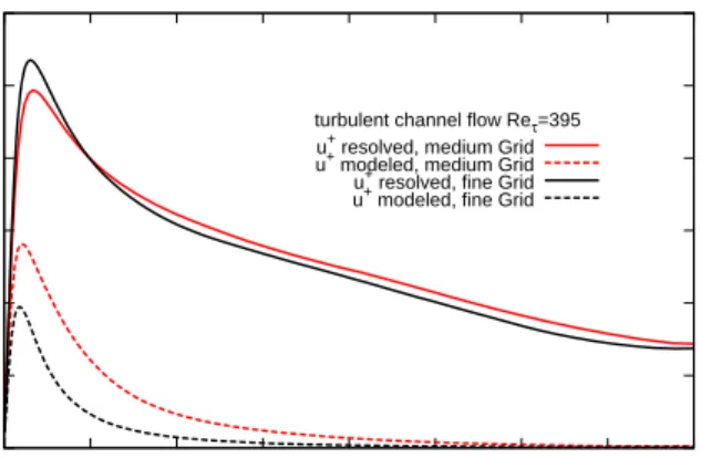
Fig. 3.1 shows the behavior of the normalized specific dissipation ωh+
close to the wall for the turbulent channel flow with Reτ = 395 obtained
with the Reynolds stress turbulence model and the DNS by Iwamoto et al.
[17] and Iwamoto [18], while two different values forCcr have been tested.
Ccr = 0.55 obtained from the asymptotic wall behavior and Ccr = 1.0
obtained by the transformation procedure fromǫh andk to ωh-equation.
As can be seen in Fig. 3.1 withCcr = 1.0 ωh+ is underestimated. While
this seems not too dramatic in Fig. 3.1, Fig. 3.2, which is just a zoom
into Fig. 3.1, reveals a certainly high underestimation. With Ccr = 0.55
the shape as well as the values ofωh+ close to the wall match the DNS.
This becomes even more obvious, if the same graph is shown for a refined mesh for the same turbulent channel flow. By clustering more points in
the viscous sublayer,ωh+ out of the simulation with the Reynolds stress
model andCcr = 0.55 follows the DNS very accurately, as can be seen in
Fig. 3.3.
One further point has to be clarified. The constant in front of the turbulent cross diffusion term 2.0νt
σ ∂ωh
∂xk
∂k
∂xk, which is basically 2.0/σ= 2.0/1.1 comes
from the direct transformation of thekandǫheq. to the ωh-eq. by using
the sameσk =σǫ, which is a simplification. Since the constants in front
of the viscous and turbulent diffusion terms should not be recalibrated, the turbulent cross diffusion allows to leave them untouched and at the same time capture the diffusion process correctly, if calibrated properly. One possible testcase for setting up the constant is the turbulent mixing layer, where the oncoming flow is divided into two parts with two different freestream velocities, a higher one and a lower one. With some distance to the inlet the flow starts to mix out which is a continuous process.
0 2 4 6 8 10 1 10 ω h+ y+
turbulent channel flow Reτ=395
JH-RSM asymptotic JH-RSM derived DNS
Figure 3.1: Close to the wall behavior of ωh+ for turbulent channel flow
withReτ= 395 - coarse grid
0 0.5 1 1.5 2 1 10 ω h+ y+
turbulent channel flow Reτ=395
JH-RSM asymptotic JH-RSM derived DNS
Figure 3.2: Close to the wall behavior of ωh+ for turbulent channel flow
3.2 Full model calculations withωh based JH-RSM 0 5 10 15 20 0.1 1 10 ω h+ y+
turbulent channel flow Reτ=395
JH-RSM asymptotic fine JH-RSM derived fine DNS
Figure 3.3: Close to the wall behavior of ωh+ for turbulent channel flow
withReτ = 395 - fine grid
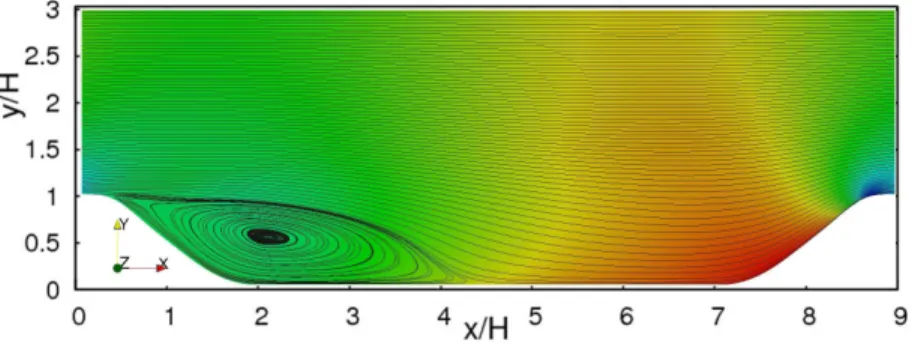
3.4 shows the computational domain presenting the already solved mean
streamwise velocity, just to give the reader a better impression. The flow is entering the domain from the left with two different velocity block profiles and an imposed velocity gradient in a small area between them.
Accord-ing to Wilcox [53], the mixing layer is an adequate testcase for setting up
the constant in front of the turbulent cross diffusion term, by matching the
spreading rate∂δ
∂xof the mixing layer, whereδ=y0.9−y0.1. y0.1andy0.9are
hereby the positions ofU =U2+0.1·∆U respectivelyU =U2+0.9·∆U (U2
is the lower inlet velocity). Table3.1shows the experimental and the
com-Figure 3.4: Streamwise mean velocity for turbulent mixing layer
puted spreading rates with 2/4 and 2/1.1 as chosen constants. Obviously
with the derived value 2/1.1, the spreading rate is highly underestimated
compared to the experiments, while 2/4 gives a spreading rate very close
in front of the turbulent diffusion, so basically 00..2591 ≈ 0.275, is close to
the results Wilcox reached [53], when he calibrated a ratio of 13//85 ≈0.208.
The ωh with the calibrated (based on the mixing layer testcase and the
Experiments JH-RSM (νt/4) JH-RSM (νt/1.1)
Spreading rates 0.0328 0.0315 0.022
Table 3.1: Spreading rates for turbulent mixing layer in self similar region asymptotic wall behavior) cross diffusion terms has the following form:
Dωh Dt = ∂ ∂xk 1 2ν+ νt σ ∂ωh ∂xk + (Cǫ1−1)ω h k Pk −(Cǫ2−1)ωhωh+2 k 0.551 2ν+ νt 4 ∂ω ∂xk ∂k ∂xk +1 kPǫ,3. (3.13)
3.2.1 Turbulent channel flow
The turbulent channel flow describes a plane channel through which a tur-bulent flow is driven by a pressure gradient. As accounted for by literature
[19] [44] [30], a lot of RANS turbulence models provide good results for a
number of flow quantities for this specific case. In the following, the new
ωh-based model will be compared to DNS data of Iwamoto et al. [18] and
Jimenez and Hoyas [24] to prove its ability to give comparably good results.
Fig. 3.5 shows the outcome in terms of the normalized mean streamwise
velocity profile for the turbulent channel flow withReτ = 395. As can be
seen the linear wall distance lawU+=U/u
τ =y+ (y+=yuτ/ν being the
normalized wall distance) fory+<5 and the logarithmic wall distance law
U+ = 1
κlny++ 5.1 for 30< y+ <100 are properly calculated. Fig. 3.6
shows the normalized Reynolds stresses, actually the normal components of the stress tensor, which are also properly calculated in peak values and
distribution, by the ωh based JH-RSM. In Fig. 3.7 the normalized
ho-mogeneous dissipation ǫh+ is plotted over y+ on two different grids, with
correct values close to the wall on both grids but the first gridpoint, which
underlines the adaptivity of theλ boundary condition, that was found to
be valid even for relatively coarse grids up to y+
≈ 4 [21]. The slightly
underestimated value of ǫh+ in the first gridpoint is not the consequence
ofωh+ in this point, sinceωh+ is by definition of the boundary condition
3.2 Full model calculations withωh based JH-RSM
kinetic energy, as can be seen in Fig. 3.8. k+is somewhat to low due to the
wrong asymptotic behavior in thevv and the ww stress component. The
same can be said forǫh+ for the higher Reynolds number (Re
τ = 2000) as shown in Fig. 3.9. 0 5 10 15 20 25 0.1 1 10 100 U + y+
turbulent channel flow Reτ=395
DNS JH-RSM log law linear law
Figure 3.5: Normalized streamwise velocity for turbulent channel flow with
0 0.5 1 1.5 2 2.5 3 0 50 100 150 200 250 300 350 400 u + v + w + y+
turbulent channel flow Reτ=395
Symbols: DNS Kasagi et al. JH-RSM
u+
v+
w+
Figure 3.6: Normalized Normal stress components for turbulent channel
flow with Reτ = 395 0 0.05 0.1 0.15 0.2 0.25 0.3 0.1 1 10 100 ε h+ y+
turbulent channel flow Reτ=395
JH-RSM coarse JH-RSM fine DNS
Figure 3.7:ǫh+ for turbulent channel flow withRe
τ= 395 - fine and coarse
3.2 Full model calculations withωh based JH-RSM 0.01 0.1 1 10 0.1 1 10 100 k + y+
turbulent channel flow Reτ=395
DNS JH-RSM
Figure 3.8: k+ for turbulent channel flow withReτ= 395
0 0.05 0.1 0.15 0.2 0.25 0.3 0.1 1 10 100 1000 ε + y+
turbulent channel flow Reτ=2000
JH-RSM DNS
Figure 3.9: ǫh+for turbulent channel flow withRe
3.3 From Rotta’s
kL
equation to the instability
sensitive model
Since the results using theωhbased JH-RSM have shown to be very
promis-ing, one can go a step further and introduce the instability sensitive term
into theωh-equation of the JH-RSM. Before doing so, some explanations
and clarifications have to be made. First of all Menter and Egorov [35]
di-rectly transformed their√kL-SAS model (√kL= Φ) toω-equation. Then
they made it fit into the SST concept. A direct transformation of the√kL
-equation to anω-equation (which in fact means to properly transform the
constants in front of the SAS part) is not preferable in the case of the
JH-RSMωhbased model for the following reasons:
• The JH-RSM uses the Reynolds stresses directly as input for the
averaged momentum equation, while all eddy viscosity models use an artificial viscosity and velocity gradients to build up the Reynolds stresses entering the momentum equation as derivatives. For that reason there is no direct general relation between the Reynolds stress modeling concept and the eddy viscosity concept.
• Normally in one and two equation models the length scale supplying
equation is set up completely empirical as a transport equation with similar structure like for example the equation for the turbulent ki-netic energy. This probably is based on the very popular and early
standard kǫ-model [31] in which the quantity epsilon was not seen
as the quantity it really is, namely the dissipation at the smallest scales, but more as a quantity representing the energy transfer from the largest to the smallest scales. One reason for that treatment, since there exists an exact equation for the dissipation rate, is the fact that this equation has a lot of lets say unsafe to model terms and no reference data for comparison was available at the very begin-ning of modeling. So turbulence researchers that time took the way to use an empirical equation which was well calibrated on different
testcases. In fact the ǫ equation in the JH-RSM is modeled out of
the exactǫequation in a term-by-term manner. The dissipation
tak-ing place at the smallest scales can be connected to the practice of modeling the whole energy transfer from the largest to the smallest scales by the fact that there can be only that amount of energy dis-sipated at the smallest scales like transferred over the whole energy cascade with bearing in mind that the energy transfer from one eddy
3.3 From Rotta’s kLequation to the instability sensitive model
to another happens only in case of eddies with similar size [19]. This
means that exactly the energy dissipated at the smallest scales must have gone through the whole transfer process. As an outcome this equation is not completely comparable quantitatively in each term
to otherǫ equations but physically as described before. Therefore a
direct transformation of the Φ-equation is not straightforward. A more convenient approach is to insert the SAS term directly from the
kω-SST-SAS model into the ωh-eq. of the JH-RSM and to calibrate it
properly, not only in terms of quantity distribution and peak values but also
by mimicking the flow behavior obtained withkω-SST-SAS. Nevertheless,
before presenting the calibration procedure the full derivation from Rotta’s
kΨ model to the ωh equation will be presented here just for the sake of
completeness. Starting with Rotta’sk and Ψ equation in boundary layer
form to estimate the constants needed for the transformation:
Dk Dt =Pk−C 3/4 µ k3/2 L + ∂ ∂y ν t σk ∂k ∂y (3.14) DΨ Dt = Ψ kPk ζ1−ζ2 L Lvk 1/2! −ζ3k3/2+ ∂ ∂y νt σΨ ∂Ψ ∂y . (3.15)
Instead of the proposed model for the term containing the second velocity derivative [34]: −163 ∂ 2U(~x) ∂y2 ∞ Z −∞ R12rydry=−const·Pk·Ψk L Lvk , (3.16)
or the newer version [35]
−163 ∂ 2U(~x) ∂y2 ∞ Z −∞ R12rydry=−const·Pk·Ψk L Lvk 2 , (3.17)
the following expression has been used:
−163 ∂ 2U(~x) ∂y2 ∞ Z −∞ R12rydry=−const·Pk· Ψk L Lvk 1/2 . (3.18)
It will be explained later why exactly this way of modeling has been chosen.
measurements of Rose [48], ζ3 ≈ 0.11−0.13 and σΨ = 1.0. ζ2 = const
can now be estimated from the logarithmic layer requirements (∂U/∂y =
uτ/κy;k = u2τ/
p
Cµ;L = κy;νt = uτκy;Pk = ǫ) [35], for example with
ζ3= 0.13: κyPkζ2=κyPkζ1−ζ3 u2 τ Cµ1/2 !3/2 +u 3 τκ2 Cµ1/2 (3.19) and finally ζ2=ζ1− ζ3 Cµ3/4 + κ 2 Cµ1/2 ≈0.97 (3.20)
withκ= 0.41 andCµ = 0.09. With the length scaleLchosen to be equal to
κyin the logarithmic layer the following expression forντ can be obtained:
ντ log =uτκy=Cντ √ kL=Cντ uτ Cµ1/4 κy. (3.21) It follows thatCντ =C 1/4
µ . For the transformation from thekΨ-model to
anω equation similar to that one from the JH-RSM model, not only the
constantζ2 has to be calculated but also the proper definition ofLhas to
be found. From the logarithmic layer requirement L = κy and from the
model for the turbulent length scale
L=CL
k3/2
ǫ =CL k1/2
ω (JH−RSM), (3.22)
it follows that CL =Cµ3/4, which is needed to be inserted in the
transfor-mation process Ψ =kL= k 3/2 ω C 3/4 µ (3.23) and consequently: ω=k 3/2 Ψ C 3/4 µ . (3.24)
By applying derivation rules
Dω Dt =C 3/4 µ Dk3Ψ/2 Dt (3.25)
3.3 From Rotta’s kLequation to the instability sensitive model
the transformation reads [9]:
Dω Dt =C 3/4 µ 3 2 k1/2 Ψ Dk Dt − k3/2 Ψ2 DΨ Dt =3 2 ω k Dk Dt − 1 Cµ3/4 ω2 k3/2 DΨ Dt. (3.26)
The simplified boundary layer form reads:
Dω Dt = ω kPk 3 2−ζ1 −ω2 32 − ζ3 Cµ3/4 ! +ω kPkζ2 L Lvk 1/2 + 3.0νt 1 k ∂ω ∂y ∂k ∂y −2.0νt 1 ω ∂ω ∂y ∂ω ∂y − 3 2νt ω k2 ∂k ∂y ∂k ∂y. (3.27)
Finally by applying a model for the productionPk =νtS2 (S =∂U/∂y is
the mean shear rate in boundary layer form), replacingνt=Cµ1/4
√ kL = Cµ1/4k 3/2 ǫ C 3/4
µ k1/2 = Cµωk and skipping the cross-diffusion term, since it
is anyway included in the transformation fromǫh to ωh, the obtained ω
-equation reads: Dω Dt = ω kPk 3 2 −ζ1 −ω2 32− ζ3 Cµ3/4 ! +CµS2ζ2 L Lvk 1/2 −2.0Cµ k ω2 ∂ω ∂y ∂ω ∂y − 3 2Cµ 1 k ∂k ∂y ∂k ∂y. (3.28)
This is basically the final expression for a transformed ω-equation from
Rotta’s model, with the term including the second velocity derivative mod-eled by Menter’s proposal. The resulting equation can be directly compared
to the transformedωh-eq. in its constants and terms. As already stated,
the cross diffusion has been skipped in the upper ω-eq. since the ωh-eq.
has a similar term. In a further stepL can be expressed in terms of the
turbulent length scale definition of the kω-SST-SAS LSST = k
1/2
Cµ1/4ω
. By simple multiplication the length scale used later can be obtained:
L= k 1/2 Cµ3/4ω =Cµ k1/2 Cµ1/4ω . (3.29)
By inserting this in eq. 3.28
CµS2ζ2 L Lvk 1/2 =C3/2 µ S2ζ2 L SST Lvk 1/2 =ζe2S2 L SST Lvk 1/2 , (3.30)
it follows thatζe2≈0.026, which is the value of the constant that is going
to be compared with the calibrated one, used in this work. Rewriting eq.
3.28leads to Dω Dt = ω kPk 3 2 −ζ1 −ω2 3 2 − ζ3 Cµ3/4 ! +ζe2S2 L SST Lvk 1/2 −CSAS Cµ k ω2 ∂ω ∂y ∂ω ∂y + 3 4Cµ 1 k ∂k ∂y ∂k ∂y , (3.31)
withCSAS= 2. During early runs with the IS-RSM, the model has shown
large numerical instabilities and needed a lot of computational effort. High order numerical schemes for the convective terms could simply not be used. With low order schemes the IS-RSM showed the same going back to RANS
mode, under locally unstable flows, like thekω-SST-SAS. The numerical
in-stability and the computational effort stems from the complicated modeled
Pǫ,3. It consists of two terms which should mimic the near wall term from
the exactǫh-eq., with changing in sign close to walls. In RANS simulations
of three-dimensional flows with no homogeneous direction in terms of mean
velocity and Reynolds stresses,Pǫ,3 consists of 108 parts. In URANS
sim-ulations with structure resolving possibility all of the 108 terms have to be used always in each timestep. This term should be modeled in a simpler way, for stability reasons as much as cost reduction. Turbulent channel
flow simulations reveal thatPǫ,3 at its peak is only 1/4 of the production
of ǫh [19]. Nevertheless it cannot be skipped since it is important for the
high value of ǫh close to the wall. An easier way to model P
ǫ,3 is not to
use eq. 3.6, but instead a kind of simple gradient approach. This has been
done in the context of modeling the near wall termE, which is important
mainly in the buffer layer [3], in the Launder-Sharma kǫ model. There it
reads: E= 2.0ννt ∂2U i ∂x2 j !2 . (3.32)
This approach will also be used from now on together with modelingPǫ,3
in the JH-RSM. The turbulent viscosity has been modeled in terms of
Reynolds stress anisotropy (see eq. 3.4). One big advantage, beyond the
much more stable behavior, is that it can be expressed with the OpenFOAM
GradGrad operator, which accelerates its computation a lot. If this term
is retransformed to its counterpart inside theǫh equation, normalized and
plotted overy+ for the turbulent channel flow withRe
τ = 395, the second
3.3 From Rotta’s kLequation to the instability sensitive model
where it is compared to the complicated form of thePǫ,3 term. The first
negative peak cannot be captured, since the GradGrad operator always
gives positive values, which is actually not so important, since very close to the wall the viscous diffusion and destruction terms make up the main parts.
The value ofǫhis captured correctly, as can be seen in Fig. 3.11, where this
quantity is plotted in its normalized form overy+ (first calculated point is
skipped). Also included in Fig. 3.11is theǫhdistribution with the skipped
Pǫ,3term, which consequently leads to an overprediction close to the wall.
-0.002 -0.001 0 0.001 0.002 0.003 0.004 0.005 0.1 1 10 100 Pε ,3 + y+
turbulent channel flow Reτ=395
JH-RSM modified JH-RSM original
Figure 3.10: Different Pǫ,3 formulations - turbulent channel flow with
Reτ= 395
A simple, robust and still, in some points away from the wall accurate
enough formulation forPǫ,3has been found, implemented and tested for the
turbulent channel in the context of Reynolds stress modeling (see Appendix A for the full model description). As a next step this is introduced into the IS-RSM. Accompanied by that, the numerical schemes for the convective
schemes are going to be increased. The finalωh-eq. of the IS-RSM has the
following form: Dωh Dt = ∂ ∂xk 1 2ν+ νt σ ∂ωh ∂xk + (Cǫ1−1)ω h k Pk −(Cǫ2−1)ωhωh+2 k 0.551 2ν+ νt 4 ∂ω ∂xk ∂k ∂xk +1 kPǫ,3+PSAS (3.33)
0 0.05 0.1 0.15 0.2 0.25 0.3 0.1 1 10 100 ε h+ y+
turbulent channel flow Reτ=395
JH-RSM w/o Pε,3
JH-RSM DNS
Figure 3.11:ǫh w/oP
ǫ,3 for turbulent channel flow withReτ = 395
with PSAS= 0.004max 1.755κS2 LSST Lvk 1/2 −8T2,0 ! , T2= k 1/3max 1 k2 ∂k ∂xj ∂k ∂xj , 1 ωhωh ∂ωh ∂xj ∂ωh ∂xj . (3.34)
The constants belonging to the instability sensitive term have been cali-brated by means of testcase computations presented in the next chapter.
e
ζ2 ≈0.026 can be compared to 0.004·1.755·κ≈0.00288 which displays
a reduction of the extra production of ωh. This is actually in line with
the expected behavior, that the Reynolds stress model can be triggered more quickly to its structure resolving mode. The original power of two at
(LSST/Lvk)2caused a high overshoot of the fluctuations with complete
de-struction of the modeled quantities. At this point it must be recalled, that the power of two was originally introduced to detect directions of homo-geneous turbulence and therefore deactivate the SAS term. In a structure resolving mode homogeneous turbulence cannot occur and so the power of two is in fact a triggering value for the SAS term, in areas where the length scale ratio is higher than one. In areas with lower length scale ratio it has a
damping function. The power of 1/2 introduced in the IS-RSM is a
mech-anism which flattens the forcing, with increasing it in areas with length scale ratios smaller then one and reducing it in areas with length scale ra-tios larger then one. This leads to an even distribution and retained proper
3.3 From Rotta’s kLequation to the instability sensitive model
modeled parts in eddy-resolving simulations, for the computed testcases (see Appendix B for the full IS-RSM description).