Passive and active flow control studies using hybrid RANS/LES methods

using hybrid RANS/LES methods

Wei Wang

Supervised by Professor Ning Qin

Department of Mechanical Engineering

The University of Sheffield

This thesis is submitted to The University of Sheffield in partial fulfilment

of the requirement for the degree of

Doctor of Philosophy

To

Thesis.

This thesis is protected by the Copyright, Designs and Patents Act 1988. No reproduction is permitted without consent of the author. It is also protected by the Creative Commons

Licence allowing Attributions-Non-commercial-No derivatives.

• A bound copy of every thesis which is accepted as worthy for a higher degree, must be deposited in the University of Sheffield Library, where it will be made available for borrowing or consultation in accordance with University Regulations. • All students registering from 2008–09 onwards are also required to submit an electronic copy of their final, approved

thesis. Students who registered prior to 2008–09 may also submit electronically, but this is not required.

Author: ... Dept: ...

Thesis Title: ... Registration No: ...

For completion by all students:

Submit in print form only (for deposit in the University Library): n

Submit in print form and also upload to the White Rose eTheses Online server: In full n

Edited eThesis n 

Please indicate if there are any embargo restrictions on this thesis. Please note that if no boxes are ticked, you will have consented to your thesis being made available without any restrictions.

Embargo details: (complete only if requesting an Embargo required? Length of embargo

embargo to either your print and/or eThesis) (in years)

Print Thesis Yes n No n _____

eThesis Yes n No n _____

Supervisor: I, the supervisor, agree to the named thesis being made available under the conditions specified above. Name: ………... ... Dept: ...

Signed: ……… ... Date: ...

Student: I, the author, agree to the named thesis being made available under the conditions specified above.

I give permission to the University of Sheffield to reproduce the print thesis in whole or in part in order to supply single copies for the purpose of research or private study for a non-commercial purpose.

I confirm that this thesis is my own work, and where materials owned by a third party have been used copyright clearance has been obtained. I am aware of the University’s Guidance on the Use of Unfair Means (www.sheffield.ac.uk/lets/design/unfair) I confirm that all copies of the thesis submitted to the University (including electronic copies on CD/DVD) are identical in content.

Name: ………... ... Dept: ...

Signed: ……… ... Date: ...

For completion by students also submitting an electronic thesis (eThesis):

I, the author, agree that the University of Sheffield’s eThesis repository (currently WREO) will make my eThesis available over the internet via an entirely non-exclusive agreement and that, without changing content, WREO may convert my thesis to any medium or format for the purpose of future preservation and accessibility.

I, the author, agree that the metadata relating to the eThesis will normally appear on both the University’s eThesis server and the British Library’s EThOS service, even if the thesis is subject to an embargo. I agree that a copy of the eThesis may be supplied to the British Library.

I confirm that the upload is identical to the final, examined and awarded version of the thesis as submitted in print to the University for deposit in the Library (unless edited as indicated above).

Name: ………... ... Dept: ...

Wei Wang Mechanical Engineering

Passive and active flow control studies using hybrid RANS/LES methods 090196432

✔

✔ ✔

Professor Ning Qin Mechanical Engineering

Wei Wang Mechanical Engineering

First and foremost, I would like to sincerely thank my supervisor, Professor Ning Qin, for his advice, support and guidance during the past four years. I have benefited a lot from his profound knowledge, illuminating suggestions, and scientific attitude. His valuable experiences and thorough knowledge on various CFD related topics influence me to become an independent scientific researcher. I deeply appreciate all of these.

I wish to express my appreciation to Dr. Franck Nicolleau for our cooperation in the study of flow through fractal orifice pipes. I would also like to thank Dr. Hongwei Zheng for his help in understanding the in-house code during the early stage of my PhD research, which laid the foundation of my four years study. I appreciate discussions with Dr. Mohammed Mohammed and Dr. Yibin Wang on numerical methods and mesh generations. I also thank Dr. Spiridon Siouris and Palma Garcia for our collaboration in the MARS project. I am here to say thank you to all of the people in our Aerodynamics Group.

I am grateful for the support of the MARS project on the investigation on ac-tive flow control, and the Leverhulme Trust for the support of study on the flow through fractal orifices. I also acknowledge the support of the EPSRC UK Turbulence Consortium, which supports the high performance computing and provides the opportunities to communicate with other groups in annual confer-ences. I appreciate the computing resources and the corresponding supporting teams, namely, Greengrid, Iceberg, HECTOR and N8. I want to acknowledge the three years’ financial support from the China Scholarship Council.

Last but not the least, I wish to devote my greatest gratitude to my whole families and friends for their enthusiastic support over the years. Especially, I would like to express my deep appreciation to my parents and my husband for their love and encouragement. Their support is the driving force in my pursuing an academic career.

Turbulent flow control of three types of flow is numerically studied using hy-brid RANS/LES approaches. Flow control effect and control mechanisms are studied through both instantaneous and statistically-averaged flow properties. Behaviours of hybrid RANS/LES methods in these three types of flow are also investigated.

Flow over a backward facing step is investigated, with piezoelectric actuators implemented on the step to control flow separation and recirculation. The simu-lation results agree well with the experiments. For the controlled flow, a slightly reduced primary recirculation between two adjacent actuators was observed. In the exploring study of actuators with a control velocity similar to the free stream flow, counter-rotating vortex pairs are generated, interacting with the separated shear layer. The primary recirculation becomes much smaller, and the recovered flow has a smaller skin friction.

Pitched and skewed jet vortex generators are applied to the NACA0015 aerofoil to study their control effect on the trailing edge separation induced by a gradual adverse pressure gradient. Both the simulation and experiments show that after a certain time, the originally separated flow is forced to be attached by the blowing jets. The lift coefficient is enhanced and the drag coefficient is reduced. When the jets are switched off, the fully attached flow recovers to the originally separated flow. The jet-removal process has about 70% longer transient time than the jet-deployment process.

Flow through fractal orifices in pipes is studied to investigate the passive control effect of the orifice geometries in flow mixing and decay. The simulation results are in good agreement with the available experimental data. With a higher fractal level, the vena contracta velocity decreases and the unrecoverable pressure loss becomes smaller. The higher level fractal orifices generate more organized vortices, maintaining a high turbulent kinetic energy for a longer distance and a slower decay. Axis-switching is observed for all these fractal orifices.

Contents iv

List of Figures x

List of Tables xxii

Nomenclature xxx

1 Introduction 1

1.1 Background and motivations . . . 1

1.2 Aims and objectives . . . 2

1.3 Outline of the thesis . . . 3

2 Literature Review 6 2.1 Introduction . . . 6

2.2 The nature of turbulence . . . 7

2.3 Flow simulation . . . 8

2.3.1 Direct numerical simulation . . . 8

2.3.2 Reynolds-averaged numerical simulation . . . 9

2.3.3 Large-eddy simulation . . . 11

2.3.4 Hybrid RANS/LES numerical simulation . . . 15

2.4 Flow control . . . 19

2.4.1 Passive flow control . . . 21

2.4.1.1 A review . . . 21

2.4.1.2 Orifice with fractal geometries . . . 22

2.4.2 Active flow control . . . 25

2.4.2.1 A review . . . 25

2.4.2.3 Fluidic flow control . . . 31

2.5 Summary . . . 41

3 Governing Equations and Numerical Methods 43 3.1 Introduction . . . 43

3.2 Assumptions in the CFD solver DG-DES . . . 45

3.3 Governing equations . . . 47

3.3.1 Unsteady Navier-Stokes equations . . . 47

3.3.2 Arbitrary Lagrangian-Euler formulation . . . 49

3.4 Temporal discretization . . . 50

3.4.1 Dual time stepping . . . 51

3.4.2 Physical time discretization . . . 52

3.4.3 Pseudo time stepping . . . 54

3.4.4 Determination of time steps . . . 55

3.5 Finite volume spatial discretization . . . 56

3.5.1 Discretisation of inviscid flux: the Roe-family flux splitting scheme . 57 3.5.1.1 Roe’s flux difference splitting scheme . . . 57

3.5.1.2 The Roe scheme with low dissipation . . . 60

3.5.2 Discretisation of inviscid flux: Simple Low-Dissipation Scheme of AUSM-family . . . 61

3.5.3 Discretisation of viscous flux . . . 63

3.6 Boundary conditions . . . 64

3.6.1 Boundary conditions for moving wall . . . 64

3.6.2 Turbulent inflow boundary conditions . . . 64

3.7 Dynamic grid techniques . . . 66

3.7.1 Discretisation of geometric conservation law . . . 67

3.7.2 Dynamic grid method . . . 68

3.7.2.1 Literatures on dynamic grid methods . . . 68

3.7.2.2 A simple dynamic grid method with a reduced moving domain 69 3.8 Techniques on Hybrid RANS/LES Turbulence Modelling . . . 71

3.8.1 Introduction . . . 71

3.8.2 Spalart-Allmaras turbulence model . . . 74

3.8.3 S-A model based DES, DDES and IDDES . . . 78

3.8.3.1 DES . . . 78

3.8.3.2 DDES . . . 79

3.8.4 Implicit LES . . . 82

3.8.5 Resolved and modelled fluctuations in LES . . . 82

3.9 Summary . . . 84

4 Flow Control with Piezoelectric Actuators in Flow Around A Backward Facing Step 85 4.1 Introduction . . . 85

4.2 Validation on flow over the BFS (Driver and Seegmiller) . . . 87

4.2.1 Introduction . . . 87

4.2.2 Flow configuration . . . 87

4.2.2.1 Computational domain . . . 87

4.2.2.2 Boundary conditions and time steps . . . 88

4.2.2.3 Mesh resolutions . . . 89

4.2.3 Comparison of results simulated with different mesh resolutions . . . 90

4.2.4 Comparison of results simulated with different flux difference splitting methods . . . 95

4.2.5 Comparison of results simulated with different hybrid RANS/LES tur-bulence modelling techniques . . . 97

4.2.6 Summary . . . 103

4.3 Flow control with piezoelectric actuators in flow over the BFS (APL-UniMan) 104 4.3.1 Introduction . . . 104

4.3.2 Flow configuration . . . 104

4.3.2.1 Description of the geometry . . . 104

4.3.2.2 Boundary conditions and time steps . . . 105

4.3.2.3 Mesh resolution . . . 106

4.3.2.4 Numerical schemes and turbulence modelling . . . 106

4.3.3 Setup of the oscillating surface in simulation . . . 107

4.3.3.1 Numerical configuration of the oscillating surface . . . 107

4.3.3.2 Control parameters . . . 109

4.3.4 Results and discussion on the baseline flow and the oscillating surface controlled flow . . . 111

4.3.4.1 Coherent vortices . . . 111

4.3.4.2 The motion of oscillation . . . 118

4.3.4.3 Flow reattachment and skin friction . . . 124

4.3.4.4 Velocity . . . 127

4.3.5 Summary . . . 136

4.4 An exploration on the control parameters of oscillating surface . . . 137

4.4.1 Introduction . . . 137

4.4.2 Results and discussion on influence of velocity amplitude . . . 138

4.4.2.1 The motion of oscillation . . . 138

4.4.2.2 Coherent vortices . . . 142

4.4.2.3 Flow reattachment and skin friction . . . 149

4.4.2.4 Velocity . . . 151

4.4.2.5 Reynolds stress . . . 156

4.4.3 Summary . . . 164

4.5 Summary . . . 165

5 Flow Control with Pulsed Jets in Flows around NACA0015 166 5.1 Introduction . . . 166

5.2 Flow configuration . . . 167

5.2.1 Description of the geometry . . . 167

5.2.2 Boundary condition and time step . . . 167

5.2.3 Mesh resolution . . . 170

5.3 Validation of turbulence models in the baseline flow of NACA0015 . . . 174

5.3.1 Introduction . . . 174

5.3.2 Comparison of DDES and IDDES in the baseline flow . . . 174

5.3.3 Summary . . . 175

5.4 Comparative study of flow characteristics in the statistically steady state of the baseline and controlled flow . . . 177

5.4.1 Coherent vortices . . . 177

5.4.2 Pressure and skin friction along the aerofoil . . . 181

5.4.2.1 The lift and drag coefficient . . . 181

5.4.2.2 The skin friction coefficient . . . 181

5.4.2.3 The pressure coefficient . . . 185

5.4.3 Controlled turbulent boundary layer . . . 188

5.4.3.1 Velocity . . . 188 5.4.3.2 Reynolds stress . . . 197 5.4.4 Wake flow . . . 209 5.4.4.1 Velocity . . . 209 5.4.4.2 Reynolds stress . . . 209 5.4.5 Summary . . . 212

5.5 Transient process of deploying and removing the jets from the baseline flow 215

5.5.1 Introduction . . . 215

5.5.2 The Cd lag zone during the transition from the baseline to jets-on . . 216

5.5.3 The large Cd fluctuations zone during the transition from a baseline flow to a controlled flow . . . 219

5.5.4 The steady zone during the transition from a baseline flow to a con-trolled flow . . . 222

5.5.5 The transition zone from jets-on to jets-off . . . 224

5.5.6 Summary . . . 225

5.6 Summary . . . 227

6 Passive Flow Control with Fractal Orifices in Pipe Flows 228 6.1 Introduction . . . 228

6.2 Validation of turbulence models in flow through a circular orifice pipe . . . . 230

6.2.1 Flow configuration . . . 230

6.2.2 Boundary condition and time step . . . 231

6.2.3 Comparison of hybrid RANS/LES turbulence modelling techniques . 232 6.2.3.1 RANS and LES zones in DES and SA-iLES . . . 232

6.2.3.2 Boundary layer . . . 234

6.2.3.3 Flow recirculation . . . 234

6.2.4 Summary . . . 235

6.3 Flow through fractal orifices . . . 238

6.3.1 Description of the geometry of fractal orifices . . . 238

6.3.2 Mesh resolution . . . 238

6.3.3 Instantaneous flow visualisations . . . 244

6.3.4 Results and discussion of statistical results . . . 251

6.3.4.1 Velocity . . . 251

6.3.4.2 Pressure drop . . . 255

6.3.4.3 Turbulence kinetic energy . . . 260

6.3.4.4 Axis-switching . . . 264

6.3.4.5 Energy spectra . . . 267

6.3.5 Summary . . . 268

6.4 Summary . . . 269

7 Conclusions 270 7.1 Summary of work, achievements and findings . . . 270

7.1.1 Performances of hybrid RANS/LES turbulence modelling in complex turbulent flow . . . 270 7.1.2 Achievements in the piezoelectric oscillating surface control of flow

over a backward facing step . . . 271 7.1.3 Achievements in the flow control with jet vortex generators in NACA0015

272

7.1.4 Achievements in the fractal orifice passive flow control in pipes . . . . 273 7.2 Suggestions for future work . . . 274

List of Published/Submitted Papers 275

2.1 Two-dimensional image of an axisymmetric water jet, obtained by the laser-induced fluorescence technique. (Prasad and Sreenivasan [1990]) . . . 7 2.2 Vorticity iso-surfaces of flow over a circular cylinder at ReD = 5×104 with

laminar separation. (a) RANS, (b) 2D URANS and (c) 3D URANS. (Spalart [2009]) . . . 12 2.3 Q-criterion iso-surfaces (coloured with the eddy viscosity ratio) by a circular

cylinder at ReD = 3.6×106. Left: URANS, Right: SAS-URANS. (Menter

and Egorov [2010]) . . . 13 2.4 Interrelation between flow control goals (Jahanmiri [2010]) . . . 20 2.5 Classification of flow control (Jahanmiri [2010]) . . . 21 2.6 Schematic view of the baseline flow in BFS (Top) and passively controlled

BFS flow (Bottom) (Neumann and Wengle [2003]) . . . 22 2.7 The first four iterations of the Koch snowflake . . . 24 2.8 The triple decomposition of a turbulence signal, cited from Hussain and

Reynolds [1970]. Upper solid curve: a turbulence signal, upper dash line: ¯

ϕ phase averaged signal and the lower curve: an organized wave. . . 27 2.9 A typical classification of flow control actuators. (Cattafesta and Sheplak

[2011]) . . . 28 2.10 Piezoelectric actuator as oscillating flap . . . 29 2.11 Piezoelectric actuator as oscillating surface. . . 30 2.12 Schematic of the SINHA Flexible Composite Surface (FCSD). (Sinha and

Ravande [2006a]) . . . 31 2.13 Schematic diagrams of synthetic jet with piezoelectric diaphragm. (Smith

and Glezer [1998]) . . . 32 2.14 Schematic diagrams of synthetic jet with (a) electrodynamic actuators (Sawant

et al. [2012]) and (b) electromechanically driven pistons (Thomas and Abra-ham [2010]) . . . 33

2.15 Schematic diagrams of steady suction with discrete orifices for laminar flow control. (Messing and Kloker [2010]) . . . 35 2.16 Flow features of steady blowing with jets into a cross flow. (Milanovic and

Zaman [2004]) . . . 36 2.17 Schematic diagrams of an unsteady blowing jets with pitched and skewed

angles. (Johnston and Nishi [1990]) . . . 39 3.1 Demonstration of the geometry similarity for the moving mesh. The top line

where the node B0 locates is the defined reduced domain range. (a) The

original geometry (b) The deformed geometry. The bottom line where the nodes A0 and its new position A locate is the moving boundary. C is an

arbitrary node with the original position C0. . . 69

3.2 Moving mesh with an oscillating surface on the boundary wall. (a) The moving mesh zone. (b) Enlarged view of the boundary mesh. . . 71 3.3 Graph of blending function fd . . . 79

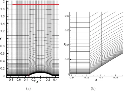
4.1 Schematic of streamlines in separation reattachement process of flows over a backward facing step (Kim [1978]) . . . 86 4.2 Experimental set up of the backward face step in Driver and Seegmiller [1985] 87 4.3 The computational domain in the x−y plane . . . 88 4.4 Computational mesh in the x−y plane of the BFS flow. Top: the whole

computational domain. Bottom: the drawing of a partial enlargement. . . . 89 4.5 Comparison of streamwise velocity with different mesh resolutions . . . 91 4.6 Comparison of modelled turbulent viscosity with different mesh resolutions. . 91 4.7 Comparison of both the modelled and the resolved Reynolds stresses with

different mesh resolutions. (a) ⟨u′u′⟩/U2

ref; (b) ⟨v′v′⟩/Uref2 ; (c) ⟨u′v′⟩/Uref2 . . . 93

4.8 Iso-surface of instantaneous vorticity magnitude. (a) Coarse mesh; (b) Fine mesh . . . 94 4.9 (a) Cf by different flux splitting methods, (b) Cp by different flux splitting

methods . . . 95 4.10 Comparison of streamwise velocity by different flux splitting methods. . . 96 4.11 Comparison of the Reynolds normal stress ⟨u′v′⟩/U2

ref by different flux

split-ting methods. . . 96 4.12 Comparison of time-averaged modelled turbulent viscosity simulated with

dif-ferent turbulence modelling. (a) DES, (b) DDES and (c) IDDES . . . 98 4.13 Profiles of modelled turbulent viscosity with different turbulence modelling. . 98

4.14 (a) Cf simulated with different turbulence modelling, (b) Cp simulated with

different turbulence modelling . . . 99

4.15 Comparison of profiles of the streamwise velocity predicted with different turbulence modelling techniques . . . 99

4.16 Comparison of both the modelled and the resolved Reynolds stresses with different turbulence modelling. (a)⟨u′u′⟩/U2 ref; (b) ⟨v′v′⟩/Uref2 ; (c) ⟨u′v′⟩/Uref2 101 4.17 The instantaneous vorticity magnitude at the central slice of the span. (a) DES, (b) DDES and (c) IDDES. . . 102

4.18 Wind tunnel model in APL-UniMan. . . 105

4.19 Computational domain in the x−y plane. . . 105

4.20 Diagram of the mesh in the x−y plane. . . 107

4.21 Experimental setup of the piezoelectric actuators. . . 108

4.22 (a) Specification of the piezoelectric actuator. (b) Diagram of the oscillating system in operation . . . 108

4.23 An example of the geometry of the oscillating surface. . . 110

4.24 Instantaneous baseline flow: the iso-surface of the three vorticity components, Ωx, Ωy and Ωz. (The light orange colour for the value of 500, and the light blue colour for the value of −500 for all these three vorticity.) . . . 112

4.25 The iso-surface of λ2 equal to -5000 for instantaneous flow. (a) Baseline flow, and (b) OS1. (The colour coding in these iso-surfaces corresponds to the streamwise velocity.) . . . 113

4.26 The iso-surface of the streamwise vorticity Ωx equal to±0.1 for instantaneous flow. (a) Baseline flow, and (b) OS1. (The colour coding in these iso-surfaces corresponds to the streamwise velocity.) . . . 114

4.27 Baseline flow: contours of the streamwise vorticity Ωx at the sections z/H = −0.346, z/H = 0, and the cross-sections x/H =−0.5, 1.0, 3.0 and 5.0 . . . . 115

4.28 The controlled flow OS1: contours of the streamwise vorticity Ωx at the sec-tions z/H = −0.346, z/H = 0, and the cross-sections x/H =−0.5, 1.0, 3.0 and 5.0 . . . 116

4.29 Power spectral density of the instantaneous pressurep(t) at (x, y, z) = (6.5,0,0) for the baseline case. (a) Experimental result of the baseline flow. (b) Simu-lation result . . . 116

4.30 Power spectral density of the instantaneous pressurep(t) at (x, y, z) = (0.2H,0.95H,0), (x, y, z) = (3H,1H,0) and (x, y, z) = (5.5H,0.4H,0). . . 117

4.31 Time-dependent motion of oscillation in one oscillating period of the control case OS1. Left: displacement of the apex of the surface. Right: vertical velocity on the apex of the surface. (The probed location and velocity are recorded every other time step) . . . 118 4.32 Four phases in the oscillating surface of one actuator . . . 119 4.33 Instantaneous velocity at the first cell above the wall in one control period.

Left column: streamwise velocityu. Middle column: vertical velocityv. Right column: spanwise velocity w. The phase angle from top to bottom: 2τ /20, 5τ /20, 7τ /20, 10τ /20, 13τ /20, 15τ /20, 17τ /20 and τ (or 0). (Note that the legends for u,v and wis different.) . . . 120 4.34 OS1: The iso-surface of the streamwise vorticity Ωx equal to ±0.05. (The

light orange colour for the value of 0.05, and the light blue colour for the value of −0.05.) . . . 121 4.35 OS1: Contours of the streamwise vorticity Ωx . . . 122

4.36 Schematic of the flow control. (a) During the vertical oscillating velocity

v <0. (b) During the vertical oscillating velocity v >0 . . . 123 4.37 Schematic of the flow control. (a) Piezoelectric actuators in this study. (b)

Passive flow control with tabs in Park et al. [2007] . . . 123 4.38 Time and spanwise averaged streamlines of the flow field. (a) the baseline

flow and (b) OS1 . . . 124 4.39 Contours of skin friction. (a) The baseline flow (b) OS1 . . . 125 4.40 Time and spanwise averaged skin friction coefficient. . . 126 4.41 Time and spanwise averaged velocities. (a) The scaled streamwise velocity

U/Ue. (b) The scaled vertical velocity V /Ue . . . 127

4.42 Time and spanwise averaged streamwise velocity. (a) at z = 0, (b) at z = 0.0225 m . . . 128 4.43 Time averaged streamwise velocity. . . 129 4.44 Time and spanwise averaged flow fluctuations. (a) The scaled streamwise

velocity fluctuations Urms/Ue. (b) The scaled vertical velocity fluctuations

Vrms/Ue . . . 130

4.45 Reynolds stress⟨u′u′⟩/U2

ref. (a) atz = 0, (b) at z = 0.0225 m . . . 131

4.46 Reynolds stress⟨u′u′⟩/U2

ref in the cross sections. . . 132

4.47 Reynolds stress⟨v′v′⟩/U2

ref. (a) atz = 0, (b) at z = 0.0225 m . . . 133

4.48 Reynolds stress⟨v′v′⟩/U_ref2 in the cross sections. . . 133 4.49 Reynolds stress⟨w′w′⟩/U2

4.50 Reynolds stress ⟨w′w′⟩/U2

ref in the cross sections. . . 134

4.51 Reynolds stress ⟨u′v′⟩/U2

ref. (a) at z= 0, (b) at z = 0.0225 m . . . 135

4.52 Reynolds stress ⟨u′v′⟩/U2

ref in the cross sections. . . 135

4.53 Schematic of the flow statistics in the mixing layer. . . 136 4.54 Time-dependent motion of oscillation in one oscillating period of the control

case OS1. Left: displacement of the apex of the surface. Right: vertical velocity on the apex of the surface. (The probed location and velocity are recorded every other time step.) . . . 138 4.55 Instantaneous velocity at the first cell above the wall in one control period.

Left column: streamwise velocity u. Middle column: vertical verlocity v. Right column: spanwise velocity w. The phase angles from top to bottom follow the time point circled in Figure 4.54. . . 140 4.56 Schematic of the velocity distribution on the first layer of cells above the

actuators. (a) Schematic of the streamwise velocity. (b) Schematic of the streamwise velocity. . . 141 4.57 Instantaneous vorticity contours at x/H = −0.5 in one control period. The

phase angles from left to right follow the time point circled in Figure 4.54. The top row for the streamwise vorticity Ωx, the middle row for the vorticity

Ωy and the bottom row for the spanwise vorticity Ωz. . . 141

4.58 The iso-surface of Ωx, Ωy and Ωz (from left to right) for OS3, OS4 and OS5

(from top to bottom). The light orange colour for the value of 500, and the light blue colour for the value of −500 for all these three vorticity components.143 4.59 The vortical structures of the jet in the cross ow in Fric and Roshko [1994] . 143 4.60 Iso-surfaces of λ2 equal to -5000 for the instantaneous flow (top view and

three dimensional view). (a) OS3 (5 m s−1_{), (b) OS4 (10 m s}−1_{) and (c) OS5}

(15 m s−1_{). . . . 145}

4.61 The iso-surface of the vorticity at the section z = 0.0225 m (left column) and

z/H = 0 (right column). (a) the streamwise vorticity Ωx, (b) the vorticity Ωy

and (c) the spanwise vorticity Ωz. . . 147

4.62 (a) The iso-surface of the streamwise vorticity Ωx at the cross sections. (b)

The iso-surface of the vorticity Ωy at the cross sections.(c) The iso-surface of

the spanwise vorticity Ωz at the cross sections. . . 148

4.63 Power spectral density of the instantaneous pressurep(t) at (x, y, z) = (6.5,0,0). From left to right: OS3, OS4 and OS5 . . . 149

4.64 Time and spanwise averaged streamlines of the flow field. (a) OS3 (5 m s−1_),

(b) OS4 (10 m s−1_{) and (c) OS5 (15 m s}−1_{) . . . 150}

4.65 Contours of skin friction. From top to bottom: OS3 (5 m s−1_{), OS4 (10 m s}−1₎

and OS5 (15 m s−1_{) . . . 151}

4.66 Time and spanwise averaged skin friction coefficient. . . 152 4.67 Time and spanwise averaged streamwise velocity. (a) at z = 0, (b) at z =

0.0225 m . . . 153 4.68 Contours of time averaged streamwise velocity the streamwise section z =

−0.0225 m and z= 0. From top to bottom: OS3, OS4 and OS5 . . . 154 4.69 Contours of time averaged streamwise velocity at the cross sectionx/H = 1.0,

3.0, 5.0, 6.5, 8.0, 10.0 and 15.0. From top to bottom: OS3, OS4 and OS5 . . 155 4.70 Reynolds stress⟨u′u′⟩/U2

ref. (a) atz = 0, (b) at z = 0.0225 m . . . 157

4.71 Reynolds stress ⟨u′u′⟩/U2

ref at the streamwise section z = −0.0225 m and z = 0. From top to bottom: OS3, OS4 and OS5 . . . 157 4.72 Reynolds stress ⟨u′u′⟩/U2

ref at the cross section x/H = 1.0, 3.0, 5.0, 6.5, 8.0,

10.0 and 15.0. From top to bottom: OS3, OS4 and OS5 . . . 158 4.73 Reynolds stress⟨v′v′⟩/U_ref2 . (a) atz = 0, (b) at z = 0.0225 m . . . 159 4.74 Reynolds stress ⟨v′v′⟩/U_ref2 at the streamwise section z = −0.0225 m and

z = 0. From top to bottom: OS3, OS4 and OS5 . . . 160 4.75 Reynolds stress ⟨v′v′⟩/U2

ref at the cross section x/H = 1.0, 3.0, 5.0, 6.5, 8.0,

10.0 and 15.0. From top to bottom: OS3, OS4 and OS5 . . . 161 4.76 Reynolds stress⟨w′w′⟩/U2

ref. (a) At z = 0, (b) at z = 0.0225 m. . . 162

4.77 Reynolds stress ⟨w′w′⟩/U2

ref at the streamwise section z = −0.0225 m and z = 0. From top to bottom: OS3, OS4 and OS5 . . . 162 4.78 Reynolds stress⟨w′w′⟩/U2

ref at the cross sectionx/H = 1.0, 3.0, 5.0, 6.5, 8.0,

10.0 and 15.0. From top to bottom: OS3, OS4 and OS5 . . . 163 5.1 Computational domain of NACA0015 (a) The x-y plane; (b) the z-y plane to

demonstrate the locations of jets . . . 168 5.2 Schematic of the experimental configuration on pulsed jets (Siauw [2008]) . . 169 5.3 Schematic of pulsed jets orientation relative to the aerofoil. . . 169 5.4 Computational mesh for NACA0015 simulation. (a) 2D mesh in the whole

domain; (b) 2D mesh near the aerofoil; (c) 3D mesh on the aerofoil near the jets’ locations; (d) 2D mesh near the leading edge; (e) 2D mesh near the trailing edge; (f) 2D near the jets’ locations. . . 172

5.5 Comparison of the first-order statistics from different mesh resolutions. (a)Time averagedCp; (b) Time averaged Cf. . . 173

5.6 (a) Instantaneous 2D streamlines at z=0. (b) Instantaneous modelled tur-bulent viscosity, and the legend stands for νt. From top to bottom: IDDES,

DDES after 0.006 s, DDES after 0.02 s. . . 176 5.7 Baseline flow: theλ2 criterion, coloured with the streamwise velocity. . . 177

5.8 Jets controlled flow att = 0.44 s after switching on the jets: theλ2 criterion,

coloured with the streamwise velocity. . . 178 5.9 Baseline flow: iso-surface of the vorticity components at ±1000 (The colour

of yellow for 1000, and the colour of blue for −1000). From top to bottom: Ωx, Ωy and Ωz. . . 178

5.10 Jets controlled flow at t = 0.44 s after switching on the jets: iso-surface of the vorticity components at ±1000 (The colour of yellow for 1000, and the colour of blue for−1000). From top to bottom: Ωx, Ωy and Ωz. . . 179

5.11 Contours of the vorticity components at ±1000 at the cross sections x/c = 0.35, 0.4, 0.5, 0.6, 0.7, 0.8 and 0.9. The left column for the streamwise vorticity Ωx, the middle column for the vorticity Ωy and the right column for

the spanwise vorticity Ωz. . . 180

5.12 Comparison of the skin friction in the baseline flow and the jets controlled flow.183 5.13 Instantaneous contours of skin friction coefficient Cf in a statistically steady

state. (a) The baseline case (the top figure for a 3D view and the bottom figure for a 2D top view); (b) The jets controlled case (the top figure for a 3D view, the bottom figure for a 2D top view and the middle figure is an enlarged view of one single jet). Note: (1) the legend of the middle figure of (b) has a different scale from others to display a clear visualization near the jets; (2) the dash line in the bottom figure of (b) represents the spanwise locations of jets. . . 184 5.14 Comparison of the pressure coefficients (both time and spanwise averaged) in

the baseline flow and the jets controlled flow. . . 185 5.15 Instantaneous contours of pressure coefficients in a statistically steady state.

(a) The baseline case (the top figure for a 3D view and the bottom figure for a 2D top view); (b) The jets controlled case (the top figure for a 3D view, the bottom figure for a 2D top view and the middle figure is an enlarged view of one single jet). Note: the dash-lines are trajectories. . . 187

5.16 Schematic of boundary layer survey direction. (a) Profile survey direction in experiments; (b) Contour survey direction . . . 188 5.17 Time averaged velocity profiles both for the baseline and the controlled cases

at (a) x= 0.846cand (b)x= 0.971c. . . 190 5.18 Contours of time-averaged streamwise velocityU for the pulsed jets controlled

flow at 10 streamwise sections fromx/c= 0.30 tox/c= 0.39. (The dash lines represent the jet locations in the spanwise direction.) . . . 191 5.19 Contours of time-averaged streamwise velocity U for the baseline flow at 10

streamwise sections from x/c= 0.30 to x/c = 0.39. . . 192 5.20 Time averaged velocity profiles at x/c= 0.32, 0.34, 0.36 and x/c= 0.38. . . 193 5.21 Time averaged velocity profiles at x/c= 0.52, 0.60 and x/c= 0.714. . . 193 5.22 Contours of time-averaged streamwise velocity U for the baseline flow at 12

streamwise sections from x/c= 0.4 to x/c = 0.95. . . 194 5.23 Contours of time-averaged streamwise velocityU for the pulsed jets controlled

flow at 12 streamwise sections from x/c= 0.4 to x/c= 0.95. (The dash lines represent the jet locations in the spanwise direction.) . . . 195 5.24 Profiles of time averaged Cf distribution in the spanwise direction at x/c =

0.4, 0.5, 0.6, 0.7, 0.8 and 0.9. (the constant line is for the pressure side) . . . 196 5.25 Mean profiles of ⟨u′u′⟩/U2

∞ both for the baseline and the controlled cases at

(a) x= 0.846c and (b)x= 0.971c. . . 198 5.26 Mean profiles of the Reynolds normals stresses ⟨u′u′⟩/U2

∞, ⟨v′v′⟩/U∞2 and

⟨w′w′⟩/U2

∞ both for the baseline and the controlled cases at x/c = 0.44,

0.52, 0.60 and 0.714. . . 199 5.27 Mean profiles of the Reynolds shear stresses⟨u′v′⟩/U2

∞,⟨u′w′⟩/U∞2 and⟨v′w′⟩/U∞2

both for the baseline and the controlled cases at x/c = 0.44, 0.52, 0.60 and 0.714. . . 200 5.28 Contours of Reynolds stresses for the baseline flow at z/c = 0. From top to

bottom, ⟨u′u′⟩/U2

∞,⟨v′v′⟩/U∞2, ⟨w′w′⟩/U∞2 and ⟨u′v′⟩/U∞2 . . . 202

5.29 Contours of Reynolds stress⟨u′u′⟩/U_∞2 for the controlled flow at 12 streamwise sections from x/c = 0.4 to x/c= 0.95. . . 203 5.30 Contours of Reynolds stress⟨v′v′⟩/U_∞2 for the controlled flow at 12 streamwise

sections from x/c = 0.4 to x/c= 0.95. . . 204 5.31 Contours of Reynolds stress ⟨w′w′⟩/U2

∞ for the controlled flow at 12

5.32 Contours of Reynolds stress⟨u′v′⟩/U2

∞for the controlled flow at 12 streamwise

sections from x/c= 0.4 to x/c = 0.95. . . 206 5.33 Contours of Reynolds stress⟨u′w′⟩/U_∞2 for the controlled flow at 12 streamwise

section from x/c= 0.4 to x/c = 0.95. . . 207 5.34 Contours of Reynolds stress⟨v′w′⟩/U_∞2 for the controlled flow at 12 streamwise

section from x/c= 0.4 to x/c = 0.95. . . 208 5.35 Profiles of time averaged streamwise velocity in the wake at x/c= 1.98. . . . 210 5.36 Contours of streamwise velocity in the wake. (a) The baseline flow (b) The

controlled flow . . . 211 5.37 Reynolds stress profiles in the wake atx/c = 1.98. (a)⟨u′u′⟩/U2

∞, (b)⟨v′v′⟩/U∞2

212

5.38 Contours of Reynolds stress in the wake for the baseline flow at z/c= 0. . . 212 5.39 Contours of Reynolds stress in the wake for the controlled flow at z/c= 0. . 213 5.40 Contours of Reynolds stress in the wake for the controlled flow flow at different

streamwise sections. From left to right at x/c = 1.1, x/c = 1.2, x/c = 1.3,

x/c = 1.4, x/c = 1.5, x/c = 1.6, x/c = 1.7, x/c = 1.8 and x/c = 1.9. From top to bottom for⟨u′u′⟩, ⟨v′v′⟩, ⟨w′w′⟩ and ⟨u′v′⟩. . . 214 5.41 The drag coefficient Cd during the whole simulation. . . 216

5.42 The drag coefficientCdduring the transient process of deploying and removal

of jets. . . 217 5.43 Top view of the flow structures represented by the λ2 criterion, coloured with

−Cp. (The red line marks where the trailing edge locates.) Left column from

top to bottom: t= 0.000 5 s, 0.003 s, 0.006 s and 0.009 s. Right column from top to bottom: 0.012 s, 0.013 s, 0.015 s and 0.018 s . . . 218 5.44 Enlarged view of the flow structures represented by the λ2 criterion, coloured

with −Cp at t= 0.013 s. . . 218

5.45 The controlled flow at t = 0.015 s and t = 0.018 s: (a) The skin friction Cf

(b) The pressure coefficient −Cp . . . 219

5.46 The drag coefficient Cd during the transient process of deploying jets. The

circled points are the sampled time steps. . . 220 5.47 The λ2 criterion, coloured with the streamwise velocity at (from top to

bot-tom) t = 0.021 s, 0.0245 s, 0.0265 s, 0.0295 s and 0.033 s. The left column is 3D view, and the right column is an enlarged side view (the red lines are references, which are perpendicular to the trailing edge surface). . . 221

5.48 Pressure coefficients during the time marching. (a) at in-between jets, z = 0, (b) at jet centre, z =λ/2 . . . 222 5.49 The contours of (a) pressure coefficient −Cp and (b) skin friction Cf, at

t = 0.021 s, 0.0245 s, 0.0265 s, 0.0295 s and 0.033 s (from top to bottom). . . 223 5.50 Skin friction during the time marching. Left: at in-between jets,z = 0. Right:

at jet centre, z =λ/2 . . . 224 5.51 The drag coefficient Cd during the transient process of removal of jets. The

circled points are the sampled time steps. . . 224 5.52 The λ2 criterion, coloured with the streamwise velocity at (from top to

bot-tom) t = 0.51 s, 0.52 s, 0.55 s, 0.6 s, 0.62 sand 0.64 s. . . 226 6.1 Computational domain of the fractal-orifice pipe. Unit: meter . . . 231 6.2 The mesh on the cross section for the circular orifice. (a) The coarse mesh

(b) The fine mesh . . . 233 6.3 The first layer y+ _{(for the coarse mesh) along the pipe wall. . . . 233}

6.4 RANS and LES regions in DES. . . 234 6.5 The velocity profiles at z/D =−2 for the coarse mesh. . . 235 6.6 The streamwise velocity along the centreline. . . 236 6.7 The modelled turbulent viscosity µt/µat z/D = 0.5, 1.0, 1.5, 2.0, 2.5, 3.0,

3.5 and 4.0. (a) Coarse mesh, DES (b) Fine mesh, DES (c) Coarse mesh, SA-ILES (d) Fine mesh, SA-ILES . . . 237 6.8 Geometry of the fractal orifices for (a) C, (b) F0, (c) F1, (d) F2 and (e) F3. 239 6.9 Mesh in the main cross section for (a) F0, (b) F1, (c) F2 and (d) F3 . . . 242 6.10 Time average streamwise velocity at the centreline for (a) C, (b) F0, (c) F1,

(d) F2 and (e) F3. Blue − − − for the coarse mesh, Red − · − · −, for the medium mesh and brown solid line for the fine mesh. . . 243 6.11 Contours of the instantaneous streamwise vorticity Ωz atz/D = 0. From left

to right: C, F0, F1, F2 and F3. . . 245 6.12 The rotation directions of the streamwise vortices just downstream of the

orifice plate (about z/D = 0) . . . 246 6.13 Contours of the instantaneous streamwise velocity w/U_∞ atz/D = 0. From

left to right: C, F0, F1, F2 and F3. . . 247 6.14 Contours of the instantaneous z-vorticity. From left to right: C, F0, F1, F2

6.15 Isosurfaces of λ2 equal to −500 000 for the instantaneous flows (only the half

part with x < 0 is shown), the colour coding corresponds to the steamwise velocity. From top to bottom: C, F0, F1, F2 and F3. . . 250 6.16 Time and space averaged velocity um/U∞ at different stations: z/D = 0.5, 1,

1.5, 2, 2.5 and 3 for (a) C, (b) F0, (c) F1, (d) F2 and (e) F3. 2, experimental data; —, simulated results. For the sake of clarity, scaling multipliers and translations have been implemented to separate the profiles in a given figure. 253 6.17 Fractal scaling effect on the centreline velocity um/U∞. (a) Experiment data

(b) Simulation results . . . 254 6.18 Contours of time-averaged normalized streamwise velocity w/U_∞ for (a) C,

(b) F0, (c) F1, (d) F2 and (e) F3. From top to bottom z/D = 0, 0.25, 0.5, 0.75, 1, 1.5, 2, 2.5, and 3. . . 256 6.19 Iso-contours of the time averaged streamwise velocity w/U_∞ in the z-y plane.

From top to bottom: C, F0, F1, F2 and F3. . . 257 6.20 Evolution of the normalized pressure drop p∗ at the pipe wall distributed in

the streamwise direction: (a) the pressure drop along the whole pipe wall, (b) enlarged view of the pressure drop in the recovery region . . . 259 6.21 Contours of the kinetic energy associated to the velocity fluctuation in the

streamwise direction, w′2/U_∞2 at the section z/D = 0, for (a) C, (b) F0, (c) F1, (d) F2 and (e) F3. . . 260 6.22 The turbulence kinetic energy, um′2/U_∞2, related with the measured velocity

fluctuations at five sections z/D = 0.5, 1, 1.5, 2, 2.5 and 3 for (a) C, (b) F0, (c) F1, (d) F2 and (e) F3. 2 experimental data; —, simulation results. Note that for the sake of comparison of the variations, scaling multipliers an translations are used at all stations. . . 261 6.23 Contours of the turbulence kinetic energy for (a) C, (b) F0, (c) F1, (d) F2

and (e) F3 at fives sectionsz/D = 0.25,0.5,0.75,1,1.5, 2, 2.5 and 3 (from top to bottom). . . 263 6.24 Contours of the turbulence kinetic energy in the z-y plane From top to bottom:

C, F0, F1, F2 and F3. . . 265 6.25 Dynamics of the azimuthal vorticity in the deformation of an elliptical ring

leading to axis switching in Hussain and Husain [1989]. . . 266 6.26 Left: schematic of vorticity distribution in a rectangular jet (Quinn [1992]).

Right: vortices by iso-surface of the vorticity magnitude flow through a rect-angular jet. (Grinstein and DeVore [1996]). . . 266

6.27 Energy frequency-spectra for the streamwise velocity fluctuations at four sta-tions: z/D = 0.5, 1, 1.5 and 2 in the centreline for (a) C, (b) F0, (c) F1, (d) F2 and (e) F3. . . 268

2.1 Flow phenomena most commonly studied in flow control . . . 20 3.1 Coefficients for the temporal accuracy . . . 53 4.1 Summary of mesh resolutions . . . 90 4.2 Mesh resolutions for the BFS (APL-UniMan) . . . 106 4.3 Control parameters of the oscillating surface . . . 110 5.1 Flow phenomena . . . 170 5.2 Summary of mesh resolutions . . . 171 5.3 Lift and drag coefficients . . . 181 6.1 Geometric parameters of the fractal orifices . . . 238 6.2 Summary of mesh resolutions . . . 241 6.3 The unrecoverable pressure loss and the pressure recovery rate . . . 258

Roman Symbols

a Speed of sound

A =Ai,(i= 1,2,3) Vector of a surface area

Aa The maximum displacement (magnitude) of the apex on an oscillating surface

Ac Conservative Jacobian matrix

C A constant number

c Chord length of an aerofoil

Cd Drag coefficient

Cf Coefficient of skin friction

CL Lift coefficient

Cp Coefficient of pressure

cp Specific heat capacity at constant pressure

CSGS A coefficient to scale the grid-spacing in a SGS model Cµ Momentum coefficient in jets flow control

cv Specific heat capacity at constant volume

D Drag force, or diameter of a pipe

d Diameter of a circular orifice in a pipe

E Specific total energy

e Specific internal energy

f Frequency

Fc Vector of convective flux

Fd Vector of dissipation flux in the Roe scheme

Fv Vector of viscous flux

H Specific total enthalpy, or height of the step in BFS

h Specific internal enthalpy

K A multiplier

k Turbulence kinetic energy

L Lift force

Le Entrance length in pipe flow

lhyb Hybrid length scale of turbulence and RANS average lRANS RANS length scale

lturb Turbulence length scale Lz Length of a span

M Mach number

n =ni,(i= 1,2,3) Normal vector of a surface

Nface Face number

nr A random number with magnitude less than a unity

Nz Cell number along a span

O Order of magnitudes

Ap Primary Jacobian matrix

Pr Prandtl number

p∗ Normalized pressure drop

Q Vector of primary variables, Q= (p, u1, u2, u3, T)T

q =qi,(i= 1,2,3) Heat flux vector

R Residual vector in the N-S equations

r A displacement vector form one point to another

R The ideal gas constant for air, R = 287.04 J Kg−1 _K−1_{, or Radius of a geometry} Re Reynolds number

Reτ Friction Reynolds number

rp Pressure recovery rate

S =Sij Rate of strain tensor, or a vector of the source term in the N-S equations

St Strouhal number, St=f L/U T Fluid absolute temperature

t Physical time

T0 The reference temperature in the Suntherland’s law,T0 = 288.15 K, or a time interval

∆t Physical time interval

∆t∗ Dimensionless time step, ∆t∗ = ∆t/(L/U_∞)

Tft Flow-through time period

ug Velocity vector on a moving surface

u =ui = (u, v, w)T,(i = 1,2,3), instantaneous velocity components in Cartesian

coor-dinates

U_∞ Free stream velocity

Ur =Uref Reference velocity uτ Friction velocity, uτ =

√

ν(∂u/∂y)

Va The maximum velocity (magnitude) of the apex on an oscillating surface

V R Velocity ratio of the control velocity to the free stream flow

W Vector of conserved variables, W= (ρ, ρu1, ρu2, ρu3, ρe,)T XR Reattachment length towards the step

x =xi = (x, y, z)T,(i= 1,2,3), Cartesian coordinates

Greek Symbols

α Thermal diffusivity, or angle of attach of an aerofoil ∆ Grid spacing in a SGS model

δ Boundary layer thickness

δij Kronecker’s delta symbol

∆τ Pseudo time step

∆xi i= 1,2,3, characteristic length of a control volume

γ Heat capacity ratio, γ =cp/cv

Γ The transformation matrix in the preconditioning

Γnc A transition format of the transformation matrix in the preconditioning

κ The von Karman constant, κ = 0.41, or thermal conductivity coefficient, or wave number

λ Bulk elasticity or second coefficient of viscosity, or spacial interval between two adja-cent jets

Λ =λk,(k= 1,2, ...5) Diagonal matrix of eigenvalues

Λc Spectral radii of the convective flux

µ Dynamic viscosity

µ0 The reference viscosity in the Suntherland’s law, µ0 = 1.7895×10−5 m−1 Kg s−1 ν Kinematic viscosity

Ω = Ωi,(i= 1,2,3) Vorticity vector

Ω Control volume

ϕ An arbitrary flow variable

Ψ A low-Reynolds number correction in DES and its variations

ρ Fluid density

τ Pseudo time, or =τij, Reynolds stress tensor

Θ A replacement of ρp in the preconditioning

θp Pitch angle

θs Skew angle

ε Coefficients in the backward Euler’s discretization

εi,j,k The Levi-Civita symbol

Superscripts

+ Dimensionless distance,y+_≡u

τy/ν

L The left side of a surface

M Modelled variables

m Time step of the pseudo time mol The modelled variables

n Time step of the physical time

′ _{Flow fluctuation}

res The resolved variables

S Sub-grid scale filtered variable

T Transposition of a vector or a matrix

tot The total variables, which is the sum of the resolved and modelled values.

Subscripts

e variables at the edge of the velocity boundary layer (99% of the freestream velocity) exp Experimental data

i i= 1,2,3, variables in the directions of the Cartesian coordinates, x, y, z j j = 1,2,3, variables in the directions of the Cartesian coordinates, x, y, z

jet Variables in the jets flow control

l variables for laminar flow

m Measured variables in experiments

m m = 1,2,3, variables in the directions of the Cartesian coordinates,x, y, z

rms Root mean square of a variable

t variables for turbulent flow

Other Symbols

ˆ· Roe averaged values

⟨·⟩ Spatial filtered, or resolved ¯· Time averaged

˜· Modified variables in the S-A model

Acronyms

2D Two Dimensional 3D Three Dimensional

ALE Arbitrary Lagranigan-Eulerian

APL-UniMan The Aero-Physics Laboratory of The University of Manchester AUSM Advection Upstream Splitting Method

BFS Backward Facing Step C The circular orifice

CFD Computational Fluid Dynamics

CFL Courant-Friedrichs-Lewy condition or number CGCL Continuous Geometric Conservation Law DDES Delayed Detached Eddy Simulation DES Detached Eddy Simulation

DGCL Discrete Geometric Conservation Law DG-DES The name of our in-house CFD solver DNS Direct Numerical Simulations

F0 The triangular orifice, the zero-level of snowflake fractal orifice F1 The first-level of snowflake fractal orifice

F2 The second-level of snowflake fractal orifice F3 The third-level of snowflake fractal orifice FCSD Flexible Composite Surface Deturbulator GCL Geometric Conservation Law

GIS Grid-Induced Separation

IDDES Improved Delayed Detached Eddy Simulation ILES Implicit Large Eddy Simulation

LLM Log-Law Mismatch LNS Limited Numerical Scales

MSD Modelled Reynolds Stress Depletion NLES Numerical Large Eddy Simulation N-S Navier-Stokes

OS Oscillating Surface

PANS Partially-Averaged Navier-Stokes

PRNS Partially-Resolved Numerical Simulation PSD Power Spectral Density

RANS Reynolds-Averaged Navier-Stokes

SA-ILES Implicit Large Eddy Simulation with Spalart-Allmaras wall modelling SAS Scale-Adaptive Simulation

SCL Surface Conservation Law SGS Sub-grid Scale

SHUS Simple High-resolution Upwind Scheme

SLAU Simple Low-dissipation Scheme of AUSM-family SST Shear Stress Transport Model

TKE Turbulence kinetic energy

URANS Unsteady Reynolds-Averaged Navier-Stokes VLES Very Large Eddy Simulation

WMLES Wall-Modelled Large Eddy Simulation ZNMF Zero Net Mass Flux

Introduction

1.1

Background and motivations

Actively or passively changing a flow field to a desired state is of immense technological importance. The purposes of manipulation of a flow field include, but not limited to, drag reduction, flow separation control, laminar-turbulent transition control, noise and vibration reduction (Gad-el Hak [2007]). Drag reduction and flow separation control are directly related to more effective transport of air, less environmental impact and increased safety in the aerospace industry. Changing or manipulating a flow field is so-called “flow control” in fluid dynamics, which is usually realized by flow control devices in a beneficial way for overall efficiency of the fluid dynamical systems (Kral [1999]). Flow control is an effective and powerful tool for improving existing fluid dynamical systems.

Since Prandtl’s boundary layer control in 1904 (Prandtl [1904]), the subject of flow con-trol has evolved into various concon-trol methods and numerous applications to fluid flows. Flow control devices can be classified into passive and active flow control methods. Passive flow control includes changing the object geometries, installing new devices to generate vortex or to break up large eddies, and so on. Active flow control has external energy introduced into flows to change original flow fields. Most of the control devices involve interacting with the boundary layer flow, to change flow properties near the wall. One popular flow control device is a vortex generator, which can be implemented through either passive or active methods. Vortex generators have been utilized on some commercial aircraft, for example, the Boeing aircraft B737 and B767. The vortex generators installed on wing upper surface or on the engine nacelles generate vortex, which interacts with the boundary layer behind the device by introducing high momentum flow from the outside of the boundary layer down to the wall surface displacing low momentum flow. Through energizing the boundary layer, vortex

generators can delay, control or even remove separation of the boundary layer, to improve lift and reduce drag. Apart from interaction with the boundary layer flow, some control devices directly force the generation of turbulence, for example, changing the geometry of the orifice in flow meters to affect flow mixing downstream. Both active and passive flow control have obtained promising control effects in recent decades.

In spite of the positive progress, there is a lack of thorough understanding of the in-teraction between various flow control devices and their manipulated flow fields. A deeper understanding can potentially improve the effectiveness of flow control. With the develop-ment of computer technology, Large Eddy Simulation (LES) has been successfully applied to complex unsteady flows at industry-relevant Reynolds numbers. In order to reduce the required mesh resolution for the boundary layer flows, Reynolds-averaged Navier-Stokes (RANS) simulation can be used in the near-wall field in the LES study, which is the hybrid RANS/LES method. Both LES and hybrid RANS/LES modelling techniques have been widely applied to complex unsteady turbulent flows, and these modelling methods have achieved reasonably good simulation results for various types of flows. These turbulence modelling techniques are also credible tools to study the interaction between control devices and their manipulated flow field without using high-cost direct numerical simulations in computational fluid dynamics (CFD). However, it is also recognized that the feasibility of LES-based simulation approaches for flow control can be further improved in terms of turbu-lence modelling, flow-control devices modelling and other related numerical issues in order to enable robust analysis of unsteady flow control problems with realistic configurations. These aspects will be systematically addressed in the present work.

Numerical investigations on flow control can provide an overall understanding of the controlled flow fields in the context of the experiments. In addition, numerical study can also explore more control device and parameters, which may inspire optimization of their control configurations and even inventions of novel control devices. Hence, this research focuses on investigating performances of various control devices and improving understandings of control mechanisms by numerical simulations of complex unsteady flow fields.

1.2

Aims and objectives

The general objective of this thesis is to study effects and mechanisms of flow control methods applied to three typical flow fields.

(1) The first one is turbulent flow over a backward facing step, which has a geometry-induced abrupt separation. Piezoelectric actuators are installed on the step before

flow separation. The oscillating motion of the actuators is expected to manipulate the boundary layer before flow separation, then to make further changes to the flow-recirculation downstream of the step.

(2) The second case is flow over a NACA0015 aerofoil at an angle of attack 11o with a mild trailing edge separation caused by the adverse pressure gradient. Fluidic jet vortex generators are implemented upstream of the separation point to control flow separation, which aims to affect the lift and drag coefficients. The above two control devices both belong to active flow control.

(3) The last case is a passive flow control, which studies pipe flow through orifices with fractal snowflake geometries. Four levels of fractal snowflakes will be simulated and compared in vortex generation, flow mixing and decay.

The main aims of the numerical investigation on all these three typical flow and corre-sponding flow control methods are summarized as follows:

• To validate turbulence modelling techniques in three classic types of flows.

• To implement numerically various control devices in the in-house CFD solver and to conduct computational simulations to extract reliable flow physics, including the first and second order flow statistics.

• To investigate the controlled flow dynamics and the interaction between the control devices and the manipulated flow field.

• To explore key control parameters and strategies for efficient flow control of dynamic fluid-structures.

1.3

Outline of the thesis

Different hybrid RANS/LES turbulence modelling techniques have their “biased” applica-tions to flow fields with different characteristics. In present work, three typical flow fields with different separation-mechanisms are studied. Under such a circumstance, a solitary chapter about flow validations may jeopardize the consistency of each studied flow type. It seems to be a more logical and natural way to organize this thesis by inserting the validation part in front of the detailed study of each baseline and flow control case. Corresponding to this arrangement, the outline of this thesis is briefly described as follows.

Chapter 1presents an introduction to flow control and turbulence modelling techniques for complex turbulent flow. Three typical flow cases with their control methods are briefly introduced. The study objectives are also described in this chapter.

Chapter 2 is a review on the published literatures and the state of the art in research on turbulent flow properties, turbulence modelling methods and flow control techniques. Turbulence modelling techniques documented in this chapter include RANS, LES, implicit LES and various hybrid RANS/LES. In the part of flow control, firstly a review of general flow control strategies and their control effect are summarized, then comprehensive reviews of the flow control devices in both experiments and numerical simulations are presented, especially piezoelectric actuators, jet vortex generators and fractal geometries.

Chapter 3 briefly introduces the in-house CFD solver, which covers the basic equations in fluid dynamics and discretization techniques in numerical simulation. Improvements of the previous in-house CFD solver and the newly added portion are presented in details, which includes the low-dissipation numerical schemes for the large eddy simulations, the hybrid RANS/LES methods based on the Spalart-Allmaras turbulence model, and the numerical realization of control methods in the in-house CFD solver, and so on.

Chapter 4 presents the numerical simulation of flow over a backward facing step at a step-height based Reynolds number of 64 000. Flow control with piezoelectric actuators with oscillating surface in this case is investigated. Firstly, a classical test case of a back-ward facing step is validated to study the mesh resolution, the numerical methods and the turbulence modelling in this abrupt separated turbulent flow. Then, flow over the backward facing step with experiments carried out by our partners in the Aero-Physics Laboratory of the University of Manchester is numerically simulated both for the baseline flow and the oscillating surface controlled flow. The numerical results are compared with the available ex-perimental data, enabling their reliable assessment. After that, more flow properties, which are not easy to be obtained from experiments, are revealed to discuss flow control effects and mechanisms. Finally, an exploring study on the flow control parameters is carried out, and the influences of the oscillation magnitudes are discussed to identify a promising control configuration.

Chapter 5 gives the numerical simulation of flow control with jet vortex generators in NACA0015 at the angle of attack 11o _{and Reynolds number about one million. Firstly,}

the application of different hybrid RANS/LES modelling techniques to this mild separation aerofoil is discussed. Then, the numerical simulation results of both the baseline flow and the controlled flow are compared with experimental data to ensure the reliability of simulations. After that, the manipulated flow field by jet vortex generators is compared with the baseline

flow field to investigate flow control effect and mechanisms. Finally, the flow dynamics during the transition process of deploying jets and removing jets are presented to obtain further understandings of the flow control mechanisms.

Chapter 6presents the numerical simulation of flow through fractal orifices in pipes at the pipe-diameter based Reynolds number of 38 900. Flow through a circular orifice pipe is validated firstly to investigate the application of hybrid RANS/LES models in this wall-bounded abruptly separated flow. After that, orifices with four snowflake fractal levels are simulated and compared with each other to study the influences of the fractal scaling effects on the pressure drop, velocity field, turbulence kinetic energy and the energy spectra.

Chapter 7 summarizes the main achievements and conclusions in the present work. Finally, recommendations for future work are suggested.

Literature Review

2.1

Introduction

For numerical investigations on turbulent flow control, there are two primary issues. One is the numerical methods with turbulence modelling, which tackles numerical realization of flow control in complex turbulent flows. The other is the flow features and mechanisms of flow control. The aim of this chapter is to present a brief introduction of a new horizon of turbulent flow modelling techniques and flow control methods.

In the review of turbulent flow modelling, firstly, the characteristics of turbulent flow are described. Then, the main turbulence modelling techniques are summarized. Feature of each modelling technique and its potential applications are discussed and compared. As the hybrid RANS/LES method is chosen as the primary modelling technique in the current study, details on the development of these hybrid methods, the improvements in the hybrid modelling, the potential problems and attempts to conquer these existing issues are discussed and summarized.

In the review of flow control, a brief description of general flow control methods is given. Passive flow control with fractal-geometry, the active flow control with piezoelectric actuators and jet vortex generators is presented in details. For each flow control method, three main parts are provided, the original concept of this control method, the status of experiments and CFD simulations, and the potential applications.

Overall, this literature review summarizes the turbulence modelling techniques, the de-velopment of flow control methods, and the numerical implementation of the turbulence modelling in flow control methods.

2.2

The nature of turbulence

This study focuses on the flow control of turbulent flows, so the characteristics of turbulence are essential. This section will briefly introduce basic features of turbulence.

Turbulent flow widely exists in nature and engineering applications. It might be smoke from a chimney, stirring coffee, running water, vapour above boiling water, a trail of streaks of condensed water vapour or wakes of an aircraft. Turbulent flow is highly nonlinear and random in nature. Even though turbulent flow is common in nature, easily generated in experiments, and simulated with numerical methods, there is no accurate definition of turbulence. Most definitions of turbulent flow are based on characteristic descriptions. Ob-serving flow through a water jet shown in Figure 2.1, the main acknowledged characteristics of turbulent flow are listed as follows (Sagautet al. [2006]).

Figure 2.1: Two-dimensional image of an axisymmetric water jet, obtained by the laser-induced fluorescence technique. (Prasad and Sreenivasan [1990])

Continuum. Turbulence is a continuum phenomenon. Even the smallest turbulent scales are much larger than molecular scales. Besides flow motion, vortices distribution is also continuous but irregular.

Irregularity. Turbulent flow is irregular and can never be reproduced in details, which makes it impossible to deterministically describe turbulent flow motions as functions of time and space coordinates. That is why most of the popular research is based on statistical methods.

Three dimensionality of the vorticity fluctuations. Turbulent flow is non-linear in its convection process, which makes flow unsteady, three dimensional and rotational with a non-zero vorticity. Vorticity dynamics plays an essential role in turbulent flows. Vortex