Information Sharing for improved Supply Chain
Collaboration – Simulation Analysis
Suganya Jayapalan
A Thesis
In the
Concordia Institute for Information Systems Engineering (CIISE)
Presented in Partial Fulfillment of the Requirements for the Degree of
Master of Applied Science (Quality Systems Engineering) at
Concordia University
Montreal, Quebec, Canada
June 2019
ii
Concordia University
School of Graduate Studies
This is to certify that the thesis prepared
By: Suganya Jayapalan
Entitled: Information Sharing for improved Supply Chain Collaboration
– Simulation Analysis
and submitted in partial fulfillment of the requirements for the degree of
Master of Applied Science (Quality Systems Engineering)
complies with the regulations of the University and meets the accepted standards with respect to originality and quality.
Signed by the final examining committee:
Dr. Jun Yan Chair
Dr. Farnoosh Naderkhani CIISE Examiner
Dr. Akshay Kumar Rathore (ECE) External Examiner
iii
ABSTRACT
Information Sharing for improved Supply Chain Collaboration
– Simulation Analysis
Suganya Jayapalan
Collaboration among consumer good’s manufacturer and retailers is vital in order to elevate their
performance. Such mutual cooperation’s, focusing beyond day to day business and transforming from a contract-based relationship to a value-based relationship is well received in the industries. Further coupling of information sharing with the collaboration is valued as an effective forward step. The advent of technologies naturally supports information sharing across the supply chain. Satisfying consumers demand is the main goal of any supply chain, so studying supply chain behaviour with demand as a shared information, makes it more beneficial. This thesis analyses demand information sharing in a two-stage supply chain. Three different collaboration scenarios (None, Partial and Full) are simulated using Discrete Event Simulation and their impact on supply chain costs analyzed. Arena software is used to simulate the inventory control scenarios. The test simulation results show that the total system costs decrease with the increase in the level of information sharing. There is 7% cost improvement when the information is partially shared and 43% improvement when the information is fully shared in comparison with the no information sharing scenario. The proposed work can assist decision makers in design and planning of information sharing scenarios between various supply chain partners to gain competitive advantage.
iv
Acknowledgements
My learning experience in this thesis has been a very remarkable one and I would like to foremost acknowledge Dr. Anjali Awasthi for her continuous guidance and mentoring. Her frequent feedback has been beneficial in improving my models, experimenting and exploring new boundaries. Thank You Professor it has been my pleasure to work with you.
Also, I would like to mention the continuous support extended by my family and friends. My parents and sister have imparted me with immense motivation and encouragement at all times. Last but definitely not the least thanks to my immediate friend Gayathri who has been around and has been my source of moral support throughout this academic journey of mine.
v
TABLE OF CONTENTS
List of Figures ... ix
List of Tables ... xii
List of Acronyms ... xiii
1 CHAPTER 1: INTRODUCTION ... 1
1.1 Background ... 1
1.2 Problem Context... 2
1.3 Thesis Objective ... 3
1.4 Thesis Organization ... 5
2 CHAPTER 2: LITERATURE REVIEW ... 7
2.1 Introduction ... 7
2.2 Supply Chain Collaboration ... 7
2.3 Information Sharing ... 9
2.3.1 Demand Information Sharing in Advance ... 11
2.3.2 Vendor Managed Inventory (VMI) ... 11
2.4 Inventory Model Decisions ... 12
2.4.1 System Structure ... 12
2.5 Simulation ... 15
2.5.1 Simulation in Supply Chain ... 15
vi
2.6 Why Discrete Event Simulation? ... 17
3 CHAPTER 3: SOLUTION APPROACH ... 21
3.1 Simulations Steps ... 21
3.2 Inventory Level and Cost Calculations ... 25
3.2.1 Demand rate and Lead Time ... 26
3.2.2 Inventory Policy ... 28
3.2.3 Inventory Costs ... 31
3.2.4 Sample (r,Q) Inventory policy Calculation ... 33
3.3 Supply Chain Collaboration - Model Conceptualization ... 34
3.3.1 No Information Sharing (NIS) ... 35
3.3.2 Partial Information Sharing (PIS) ... 39
3.3.3 Full Information Sharing (FIS) ... 44
4 CHAPTER 4: DES MODEL TRANSLATION IN ARENA ... 46
4.1 Elements of the Simulation Model ... 46
4.1.1 System: ... 47
4.1.1.1 New Simulation Creation ... 47
4.1.2 Events: ... 48
4.1.2.1 Events - Entity Creation ... 49
4.1.2.2 Events - Delay Module ... 49
vii 4.1.3 Entities: ... 51 4.1.3.1 Entity Information ... 51 4.1.4 Attributes: ... 52 4.1.4.1 Attribute Information ... 52 4.1.5 Variables: ... 53 4.1.5.1 Variable Information ... 53 4.1.6 Queues: ... 54 4.1.6.1 Queue Information ... 55 4.1.7 Expression Information ... 56
4.2 Variable, Attribute, Queues - Arena Simulation Model ... 57
4.3 Replication Parameters tab Setup ... 59
4.4 (r,Q) Model Explanation ... 60
4.5 Information Sharing model ... 64
4.5.1.1 No Information Sharing model ... 65
4.5.1.2 Partial Information Sharing model ... 69
4.5.1.3 Full Information Sharing model ... 71
4.6 Process Analyzer Output ... 73
5 CHAPTER 5: NUMERICAL ILLUSTRATION ... 76
5.1 Model Verification ... 77
viii
5.2.1 Scenario 1 – NIS ... 83
5.2.2 Scenario 2 – PIS ... 85
5.2.3 Scenario 3 – FIS ... 87
5.2.4 Sensitivity Analysis ... 90
6 CHAPTER 6: CONCLUSIONS AND FUTURE WORKS ... 92
6.1 Conclusion... 92
6.2 Future Works ... 93
7 REFERENCES ... 94
A APPENDIX A ... 108
A1 No Information Sharing – Excel Spread sheet ... 108
A2 Partial Information Sharing – Excel Spread sheet ... 109
ix
List of Figures
Figure 1: A Typical Supply Chain (Source: Chang and Makatsoris, 2001) ... 2
Figure 2: Information Sharing Scenario ... 5
Figure 3: The scope of collaboration: generally (Source: Barratt M, 2004) ... 8
Figure 4: Inventory Model Decisions ... 12
Figure 5: General Arborescent Systems (Source: Hopp and Spearman, 2011) ... 13
Figure 6: Arborescent Series – Two Stage System ... 14
Figure 7: Literature Work - IS Methodologies -Graph ... 20
Figure 8: Solution Approach ... 21
Figure 9: Simulation Process ... 24
Figure 10: (Q,r) inventory model with Q=4 and r=4 (Source: Hopp and Spearman, 2011) ... 29
Figure 11: Inventory level and Cost Calculation Example. ... 34
Figure 12: No Information Sharing (NIS) ... 36
Figure 13: Order flow in two-stage system (Source: Tee & Rossetti, 2003) ... 36
Figure 14: No Information Sharing (NIS) – Swimlane Diagram ... 38
Figure 15: Partial Information Sharing (PIS)... 40
Figure 16 : Case 0: Order delivery time > Ls ... 41
Figure 17 : Case 1: 0 < Order Delivery Time < Ls ... 42
Figure 18 : Partial Information Sharing (PIS) - Swimlane Diagram ... 43
Figure 19 : Full Information Sharing (FIS)... 44
Figure 20 : Full Information Sharing (FIS) - Swimlane Diagram ... 45
x
Figure 22 : Arena Run Setup ... 48
Figure 23 : Entity Creation ... 49
Figure 24 : Delay Module ... 50
Figure 25 : Hold Module... 51
Figure 26 : Entities Information in Arena ... 52
Figure 27 : Attribute Information in Arena... 53
Figure 28 : Variables Information in Arena ... 54
Figure 29 : Queue Information in Arena... 56
Figure 30 : Expression Information in Arena ... 57
Figure 31 : Run Setup – Replication Parameters Tab ... 59
Figure 32 : Filling Logic (Model Source: Rossetti, 2015) ... 61
Figure 33 : Back Ordering Logic (Model Source: Rossetti, 2015) ... 63
Figure 34 : Replenishment Logic (Model Source: Rossetti, 2015) ... 64
Figure 35: Performance Measure collection Logic (Model Source: Rossetti, 2015) ... 64
Figure 36: Retailer Logic ... 66
Figure 37: Warehouse Logic ... 67
Figure 38: Expression Block ... 68
Figure 39: Expression Value Dialogue in Expression Block ... 69
Figure 40: Statistic Block... 69
Figure 41: ADI check logic... 70
Figure 42: Due date delivery logic... 71
Figure 43: (Model Adapted: Rossetti, 2015) ... 72
xi
Figure 45: Scenario Property ... 74
Figure 46: Scenario, Controls, Response ... 75
Figure 47: NIS – Arena Report ... 78
Figure 48: PIS – Arena Report... 80
Figure 49: FIS – Arena Report... 82
Figure 50: NIS – Validation ... 84
Figure 51: NIS – Validation for 50 Reps ... 85
Figure 52: PIS – Validation ... 87
Figure 53: PIS – Validation for 50 Reps ... 87
Figure 54: FIS Validation ... 89
Figure 55: FIS Validation for 50 Reps ... 89
xii
List of Tables
Table 1: Benefits of Information Sharing (Adapted from: Lotfi et al., 2013) ... 10
Table 2:Literature Work - IS Methodologies ... 19
Table 3:Literature Work - IS Methodologies - Summary ... 20
Table 4: Fill rate for respective R values ... 33
Table 5: Variables, Attributes and Queues - Arena Definition ... 58
Table 6: NIS Verification... 77
Table 7: PIS Verification ... 79
Table 8: FIS Verification ... 81
Table 9: NIS – Input and Output Parameters ... 84
Table 10: PIS – Input and Output Parameters ... 86
Table 11: FIS – Input and Output Parameters ... 88
xiii
List of Acronyms
Acronym Description
DES Discrete Event Simulation EDI Electronic Data Interchange
CPFR Collaborative Planning, Forecasting and Replenishment JIT Just In Time purchasing
VMI Vendor Managed Inventory IS Information Sharing
ADI Advance Demand Information Sharing NIS No Information Sharing
PIS Partial Information Sharing FIS Full Information Sharing
TC Total Costs
SCM Supply Chain Management
DC Distribution Center
WH Warehouse
1
1
CHAPTER 1:
INTRODUCTION
1.1 Background
In order to stay competitive in the market, most organizations are gradually understanding the need for collaboration among different supply chain entities. Consistent higher profits and end customer satisfaction are the key driving factors for an efficient supply chain and a collaborated supply chain is an undeniable solution towards it (Srivathsan & Kamath, 2018). Among the many frameworks and strategies available for collaboration, Information Sharing within the supply chain is found to have reaped considerable benefits. Advent of technology like electronic data interchange (EDI) has aided this concept and the supply chain members find it fruitful when integrated together. When it comes to collaborative techniques, organizations are looking forward to adopt tools like collaborative planning, forecasting and replenishment (CPFR), just in time purchasing (JIT) and vendor managed inventory (VMI) (Park et al., 2010). Once the collaboration strategy is identified, the right information can be shared up the stream, bringing down any risks and uncertainties while expanding profits and customer satisfaction. There are many information's that is beneficial when shared across the chain, but the demand is the most significant one. The thesis addresses this topic and studies how the total costs decrease when demand as an information is shared.
Simulation is about replicating the real-world events over time using computer or physical models. Simulation models have been used to understand the processes in many domains like healthcare, aeronautical, etc. including supply chains (Rossetti, 2015). Inventory management in a supply chain is a very important but complex process particularly with stochastic demand from consumers. It can be modelled as discrete or continuous distribution making it an ideal entity to be evaluated via
2
simulation. There are various simulations in use nowadays but a stochastic consumer demand in supply chain could be well studied via Discrete Event Simulation. Also, Arena being a popular simulation tool, is identified and used for modeling the supply chain collaboration models.
1.2 Problem Context
According to (Chang and Makatsoris, 2001) the phrase Supply Chain Management came up in the
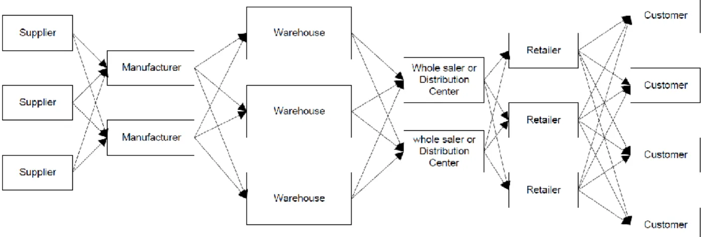
early 1990’s as a process of integrating the supply chain members so that the goods are produced in the right amount, at the right place, at the right time while in parallel satisfying the customer and keeping the cost to the minimum. A typical supply chain is presented in Figure 1. It consists of various organizations involved from the supplier to the customer (Chang and Makatsoris, 2001).
Figure 1: A Typical Supply Chain (Source: Chang and Makatsoris, 2001)
(Faisal et al, 2006) suggest that a traditional supply chain system does not focus on waste elimination. They further share that traditional supply system meets uncertainties in its information or material flow by means of buffer goods which is met at higher costs and are very slow in its
3
response to demand changes. The authors advocate that these issues are mainly due to the lack of collaboration and information sharing between the supply chain members.
From the typical supply chain network understanding from (Chang and Makatsoris, 2001), it is very evident that a supply chain network is highly complex in nature and if not managed appropriately could lead to two main issues of high cost which in turn result in a low profit and unsatisfied customers which may basically lead to lost business/sales.
Also, from (Faisal et al, 2006) studies, traditional supply chain incurs high cost and lost customer satisfaction as they work as independent entities with no information sharing between them. This thesis will demonstrate how a collaborated supply chain, with sharing of information up the stream is able to minimize its operational cost, which could also thereby eventually transform a traditional supply chain network to an agile supply chain network.
1.3 Thesis Objective
This thesis intent would be to demonstrate the value increase in the supply chain when the level of collaboration is improved. With Demand as the control factor, the total cost reduction in the supply chain is studied. Discrete Event Simulation (DES) methodology is applied and an analysis of the performance parameters based on the input controls is done. The simulation models shall output supply chain performance with collaboration at three levels as shown in Figure 2:
No Information Sharing (NIS): There is no flow of any Information from the Retailer to the Warehouse. The Warehouse receives its orders from the retailer whenever it is reorder time for the retailer. This model is considered as the Baseline Model.
4
Partial Information Sharing (PIS): Here there is a Partial Information Share from the Retailer to the Warehouse. The Consumer demand is given to the Warehouse in advance before the retailer places his order with the Warehouse.
Full Information Sharing (FIS): Here the consumer demand is placed directly to the Warehouse and retailer becomes a facilitator. Warehouse takes full control of the information and replenishes the order.
In addition, the models implemented would give a reasonable view on • how traditional supply chain efficiency could be improved
5
Figure 2: Information Sharing Scenario
1.4 Thesis Organization
This thesis has been structured in the following manner:
Chapter 2 – provides literature on the topics of supply chain collaboration, information sharing, queue information sharing, vendor managed inventory, discrete event simulation and Arena.
6
Chapter 3 – presents the solution approach. It covers the discrete event simulation process, conceptual model and detailed steps in which the simulation model was executed and results generated.
Chapter 4 – presents the model adaptation and implementation in Arena. This chapter provides all necessary information on how the model was adapted and executed using the Arena software all steps and procedures with respect to it has been explained here.
Chapter 5 – presents the numerical evaluation. The models developed are evaluated by a case study. Detailed numerical example and verification and validation of the model results are provided. Also, the sensitivity analysis is included to determine the impact of input parameters on final results.
Chapter 6 – presents the conclusion and future works. This section gives the final summary of the research in connection to the objective and on topics of future research.
7
2
CHAPTER 2:
LITERATURE REVIEW
2.1 Introduction
In this chapter, research available on the topic is reviewed and discussed. Section 2.2 describes the supply chain collaboration. Section 2.3 discusses Information Sharing and how it is seen as key enabler to supply chain collaboration. This section further elaborates on two topics, one being advance information sharing (a priori) which helps in partial collaboration and the other topic is on vendor managed inventory which is aligned to a full collaboration scenario. In section 2.4 the research and available information on inventory model decisions has been vividly detailed. Finally, section 2.5 brings out the literary work with respect to why discrete event simulation, since the approach has been embraced as a methodology is used to evaluate the objective.
2.2 Supply Chain Collaboration
Industries seeking to be ahead in the competitive world, have been evolving, by adopting new methodologies as early as from the nineteen century. In that era, work process integrations and optimizations were brought in by concepts such as lean production or just-in-time (Hopp and Spearman, 2011). After that supply chain collaboration has been the norm to share knowledge and to work integrated for an effective flow of products to the consumers (Caridi et al., 2005)
(Simatupang and Sridharan, 2002) in their research have defined supply chain collaboration as two or more supply chain member operating together by means of information sharing, mutually sharing benefits and looking to take joint decisions, so that high profits could be gained coupled together with greater level of end customer satisfaction.
8
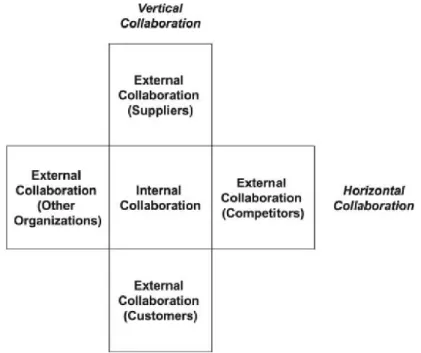
There are different ways in which collaboration could happen and there are two distinct categories under which they could be encompassed - as per the review done by (Barratt, 2004). The first one is the vertical collaboration which includes the internal collaboration within supply chain members and external collaboration with suppliers or customers. The second one is horizontal collaboration which includes the collaboration between the external competitors or other organizations (Barratt, 2004).
Figure 3: The scope of collaboration: generally (Source: Barratt M, 2004)
He has understood this flow from research done by (Simatupang and Sridharan, 2002) and consolidated it in in Figure 3 (Barratt, 2004). The thesis shall focus on internal collaboration which is a collaboration between the internal supply chain functions only.
Supply chain collaboration however is greatly challenged by the ever-fluid state of the global economic conditions, which leads us to believe whether it is successful or not (Magnan and
9
Fawcett, 2002). From the various surveys and case study interviews, it is understood that very few companies have been able to integrate their supply chain successfully, also their study indicates that there are gaps between the theoretical and the ideal world (Magnan and Fawcett, 2002). (Kohli and Jensen, 2010) had undertaken to measure the effectiveness of collaboration by studying the existing available literature and among their various inferences, a conclusion states that the effectiveness of collaboration is perceived to be high when there is information sharing between the supply chain members which leads the chapter to discuss more on information sharing further.
2.3 Information Sharing
(Simatupang and Sridharan, 2002) describe information sharing as the bidirectional flow of information between the supply chain members thereby giving all the necessary insight across the internal functions and organizations. The authors also clarify that information sharing across the members lead to high customer service.
When it comes to what type of information could be shared, (Lotfi et al., 2013) there are many types such as on logistics, business, strategic, tactical and so on. The authors have also mentioned information categories such as 1) Inventory Information; 2) Sales Data; 3) Sales Forecasting; 4) Order Information; 5) Product Ability Information; 6) Exploitation Information of New Products; and 7) Other Information (Lotfi et al., 2013).
(Lotfi et al., 2013) have researched in detail and came up with a comprehensive table summarizing the benefits of information sharing in supply chain. Table 1 is an extract from their research that gives a good view on the benefits reaped when there is information sharing in the chain. Also, further benefits as reviewed has been adapted and presented in the table 1.
10
S.Nos Benefits Sources
1 Inventory reduction and efficient inventory management (Prakash et. Al., 2010)
2 Cost reduction (Prakash et. Al., 2010)
3 Increasing visibilities (significant reduction of uncertainties) Ali et al., 2017 4 Significant reduction or complete elimination of bullwhip effect
(Hussain & Saber,2012) (Jauhari,2009)
5 Improved resource utilization (Mourtzis,2011)
6 Increased productivity, Organizational efficiency and improved
services (Singh,2015)
7 Sustainable supply chain - Decisions based on environment (Khan et. al., 2016)
8 Early problem detection (Jauhari,2009)
9 Quick response (Jauhari,2009)
(Mourtzis,2011)
10 Reduced cycle time from order to delivery (Singh,2015)
Table 1: Benefits of Information Sharing (Adapted from: Lotfi et al., 2013)
(Yan et al.,2001) have demonstrated on how cost and inventory level reduces when the information sharing between the retailer and manufacturer is gradually increased. The authors have found that there is a pareto improvement which means that all members have benefited, and some members have strongly benefited in terms of cost saving when information share level is increased in steps. (Gaur et al., 2005) have explored on how when demand has an information when shared up the stream in a two-stage supply chain model by the retailer to the manufacturer, lead to significant benefits like the safety stock reduction at the manufacturer side. This study implies that demand as information share is found to lead to substantial benefits not only to the manufacturer or retailer but also to the overall supply chain system.
11
2.3.1 Demand Information Sharing in Advance
This chapter has adapted partially the concept of demand information in scenario 2 of the partial information sharing system. So, reviews carried out on it are as below:
(Hariharan and Zipkin, 1995) studied the supply chain system performance when the customer demand information is received in advance. They have developed a model describing it and the output analysis from the model is that the ‘demand lead time’ improves the performance of the
system whereas the ‘supply lead time’ worsens it. Their study also exposes that this early information is a substitute for supply lead time and if managed well could reduce the safety stock and its corresponding cost in the supply chain system.
(Karaesmen et al., 2013) propose that if the advance demand information is handled effectively then the production/inventory performance would gradually increase. They have derived prepositions which tell us on which scenarios the advance information received could be meaningful and generate more benefit.
2.3.2 Vendor Managed Inventory (VMI)
(Marques et al., 2010) has studied the concept of VMI from concept to process and summarizes on the operational and collaborative element in VMI. According to the authors, VMI is a supply chain integration where in the focus is on the continuous replenishment of the customers inventory. They also say that the partners share demand, requirements and constraints so they can have a shared objective.
(Yao et al., 2007) evolved a mathematical model for a single-vendor single-retailer VMI system. The demand information is assumed to be deterministic and the model carried an analysis on the cost performance between a system with VMI and a system without VMI. Results reveal that the
12
benefits are found to be spread between the buyer and the supplier in an uneven manner. But in alignment to existing literatures, (Yao et al., 2007) found that implementation of VMI does reduce the inventory cost of the system thus rendering it to be beneficial.
2.4 Inventory Model Decisions
In a supply chain, a key aspect that establishes the health of the system is the inventory management. The financial upturn or downturn is very much determined by the inventory management decisions. It not only impacts a member in the chain, it affects in all layers. Hence maintaining an optimum value of inventory in a system supports the fiscal growth of the organization. In this thesis the decisions for an inventory model has been considered as per the Figure 4.
Figure 4: Inventory Model Decisions
2.4.1 System Structure
System Structure is about the distribution structure of a firm. It varies greatly from industry to industry and based on the nature of the product and the consumer demand patterns. It could be
13
considered as a system configuration which is a key and fundamental start point to an inventory model decision. Based on the storage location of inventory in a system there is Single Stage or Multi Stage system. There could be single or multiple products as output from this system. But the total quantity produced is strongly dependent on the production capacity, cost allocations and demand received from consumers.
Arborescent System are those systems in which each inventory location is served by a single source. Two networks in it could be the Serial State Network and the Multi Level Network (Figure: 5) (Hopp and Spearman, 2011)
Figure 5: General Arborescent Systems (Source: Hopp and Spearman, 2011)
In the serial system there are many stocking sites in series and each site serves only one destination site. Usually supply is also from a single source. In the multilevel arborescent system, the stocking sites may supply to more than one destination and there is multi level in it.
14
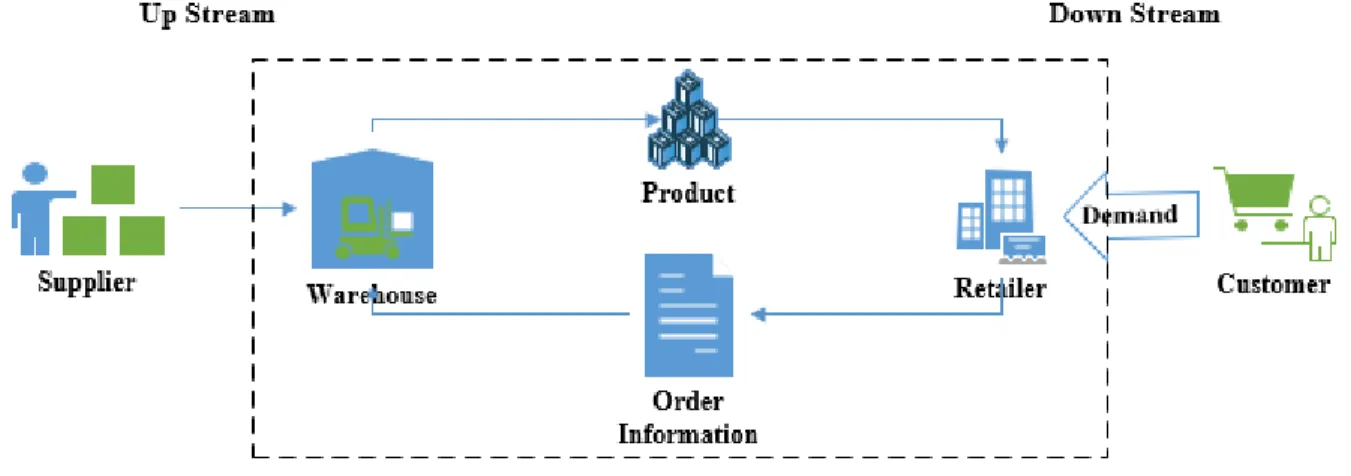
In supply chain, the member close to the customer is said to be down the stream and the member close to the supplier is up the stream. Down the stream the demand information is understood from the consumers and produce is supplied as required to them. Upstream the procurement from the suppliers on raw material required is carried out so it can be used for manufacturing or distribution to the retailers who in turn supply to the customers. Information flow in this supply chain is always up the stream and the goods flow down the stream. Figure 6 is represented to show clearly on upstream and down stream in a two-stage network system.
Figure 6: Arborescent Series – Two Stage System
Also, the network system that this chapter shall consider would be the series two stage system as depicted in Figure 6. The goal of the thesis is to simulate and understand the benefits when the collaboration among the members is improved gradually, so the idea is that if initially in a series system the outputs are achieved exploring it further with multi level could be progressive.
15
2.5 Simulation
According to (Banks et al., 2010), simulation is an approach to study systems in the conceptual phase before implementation, thus it can serve as either an analysis tool to know in advance about the impacts in incorporating changes to existing system or as a design tool to know the performances of the new design in under varying conditions.
(Kelton and Barton, 2003) have conveyed on how a carefully planned simulation could yield valuable information with any undue computational time or efforts. In the simulation context, they have shared on some ideas, challenges and opportunities when looking to model and study behaviour patterns from the simulation models.
Also, model is defined as a system’s representation in order to study the system in detail, where
the system is clarified to be a group of objects that work together in a known pattern of interaction or in some interdependence with each other so that a common objective is met. So, the term modelling is the process of creating this representation of the system (Banks et al., 2010).
The thesis models are generated with the view that the supply chain system could be studied so that by measuring its performance the operations could be improved and redesigned to capitalize on the benefits.
2.5.1 Simulation in Supply Chain
For many years, analytical modeling has been the tool which has been used by management for supply chain, but it was more theoretical and did not solve practical problems. In this context (Swaminathan et al., 1996) has reviewed that Simulation has gained considerable attention and momentum. The authors have also identified various purposes when using modeling and simulating a supply chain system. The result of their research evidently depicts on how analytical
16
results could be coupled with simulation and the model by itself is able to serve as a tool for decision making to industries. (Swaminathan et al., 1996).
Managing a complex supply chain is very much necessary, so that a business can thrive
successfully in today’s scenario. Understanding the impact of a company’s policy on the supply
chain is not likely to be known before the role out of the policy. Here the supply chain simulation models facilitate to bridge this gap. Mathematical model or Analytical may have proven success in getting the results if at the system was simple but for real life complex problems studying the system via simulation would be the best. (Law and Kelton, 2000)
2.5.2 Discrete Event Simulation
As per (Rossetti, 2015), simulations could be classified from perspective of time as static or dynamic, stochastic or deterministic and discrete or continuous. The author further details, a static system to be a system which is constant over time and a dynamic system evolves over time. Also, the system if found to be random in nature then it is stochastic else it is considered as a deterministic system. From a function of time standpoint, (Rossetti, 2015) clarifies that discrete systems are those that have their state changes at discrete point in time whereas in continuous system the state changes occur continuously. He further explains that in a discrete event simulation when a specific change happens in the system, observations are collected at that point in time but in continuous event simulation the observations are collected continuously over the period. In this thesis, the focus of the discrete simulation event model would be stochastic and dynamic in nature. Discrete Event Simulation gives the opportunity to evaluate the operating performance in advance to the implementation of the actual system. What-if analysis could be carried out by the companies which aides them in efficient decision making with such models. Also, various operational alternatives could be identified from these models without disturbing the existing systems for a
17
better policy decision (Chang and Makatsoris, 2001). The authors have also mentioned that prior to start of the supply chain modeling one should be aware of the entire supply chain. Also identifying the correct performance measure is vital. (Chang and Makatsoris, 2001).
2.6 Why Discrete Event Simulation?
In order to understand the various methodologies used to evaluate information sharing in a supply chain, the last ten years literary work has been reviewed and summarised in table 2. Google Scholar was used to find the papers. The top results with respect to each year has been captured and reviewed.
Author Year Topic Methodology
Jiang and
Ke 2019
Information sharing and bullwhip effect in smart destination
network system Mathematical
Kiyoung and
Jae-Dong
2019 The impact of information sharing on bullwhip effect reduction in a supply chain
Simulation Raweewan
and Ferrel 2018 Information sharing in supply chain collaboration Other Srivathsan
and Kamath
2018 Understanding the value of upstream inventory information sharing in supply chain networks
Mathematical Li et. al. 2018 Information and profit sharing between a buyer and a supplier:
Theory and practice Other
Dominguez
et. al. 2018
OVAP: A strategy to implement partial information sharing
among supply chain retailers Simulation
Zhao et. al. 2018 What is the value of an online retailer sharing demand forecast
information? Mathematical
Ali et. al. 2017 Supply chain forecasting when information is not shared Other Zaheer and
Trkman 2017
An information sharing theory perspective on willingness to
share information in supply chains Other
Minkyun and Sangmi
2017
The impact of supplier innovativeness, information sharing and strategic sourcing on improving supply chain agility: Global supply chain perspective
Other Haobin et.
al. 2017
Enhancement of supply chain resilience through inter-echelon
18
Khan et. al. 2016 Information sharing in a sustainable supply chain Mathematical Wenliang
et. al. 2016 Two-way information sharing under supply chain competition Other Pan et. al. 2016
Revisiting the Effects of Forecasting Method Selection and Information Sharing Under Volatile Demand in SCM Applications
Mathematical Choudhary
et. al. 2016
VMI versus information sharing: an analysis under static
uncertainty strategy with fill rate constraints. Mathematical Rached et.
al. 2016
Decentralized decision-making with information sharing vs.
centralized decision-making in supply chains Mathematical Rached et.
al. 2015
Assessing the value of information sharing and its impact on
the performance of the various partners in supply chains Mathematical Salvatore
et. al. 2015
A simulation model of a coordinated decentralized supply
chain Simulation
Costantino
et. al. 2015
The impact of information sharing on ordering policies to
improve supply chain performances Simulation
Giloni
et.al. 2014
Forecasting and information sharing in supply chains under
ARMA demand Mathematical
Cannella
et. al. 2014 An IT-enabled supply chain model: a simulation study Simulation Cigolini et.
al. 2014
Linking supply chain configuration to supply chain
performance: A discrete event simulation model. Simulation Yan et. al. 2014 Intelligent Supply Chain Integration and Management Based
on Cloud of Things Other
Ming et. al. 2014 Demand information sharing and channel choice in a
dual-channel supply chain with multiple retailers Mathematical Inderfurth
et. al. 2013
The Impact of Information Sharing on Supply Chain
Performance under Asymmetric Information Other
Fei and
Zhiqiang 2013
Effects of information technology alignment and information
sharing on supply chain operational performance. Other Jin Kyung
Kwak 2013
Comparison of (s, S) and (R, T) Policies in a Serial Supply
Chain with Information Sharing Mathematical
Lin and
Shayo 2012
Systems Dynamics Modeling for Collaboration and
Information Sharing on Supply Chain Performance and Value Creation
Simulation Yang Feng 2012 System Dynamics Modeling for Supply Chain Information
Sharing Simulation
19 Taho et.Al. 2011
Evaluation of robustness of supply chain information-sharing strategies using a hybrid Taguchi and multiple criteria
decision-making method
Other Saxena et.
al. 2010
Simulation-based decision-making scenarios in dynamic
supply chain Simulation
Prakash and
Deshmukh 2010
Horizontal Collaboration in Flexible Supply Chains: A Simulation Study
Simulation Bottani and
Montanari 2010 Supply chain design and cost analysis through simulation. Simulation Yu et. al.
2010
Evaluating the cross-efficiency of information sharing in
supply chains Simulation
Mei et. al.
2010
Supply chain collaboration: conceptualization and instrument
development Other
Li and Hau 2009 Information Sharing and Order Variability Control
Under a Generalized Demand Model Mathematical
Jain et. al. 2009 Enhancing flexibility in supply chains: Modelling random
demands and non-stationary supply information Mathematical Chan and
Chan 2009 Effect of information sharing in supply chains with flexibility Simulation Saxena et.
al. 2009
Flexible configuration for seamless supply chains: Directions
towards decision knowledge sharing Simulation
Table 2:Literature Work - IS Methodologies
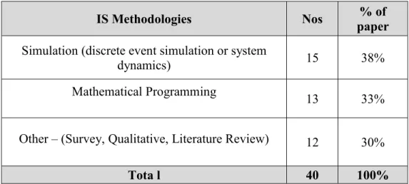
The literary work has then been categorized per the research methodology. Table 3 shows the results distribution. It can be seen that simulation scores the highest followed by mathematical optimization models and others which includes approaches like game theory, theoretical framework, survey-based framework etc.
20
IS Methodologies Nos paper % of
Simulation (discrete event simulation or system
dynamics) 15 38%
Mathematical Programming
13 33%
Other – (Survey, Qualitative, Literature Review) 12 30%
Tota l 40 100%
Table 3:Literature Work - IS Methodologies - Summary
Figure 7 gives a graphical representation for a better understanding. Compared to all other
methodologies’ simulation is found to be more adaptive and suitable for this objective compared to other approaches. Hence, discrete event simulation has been adopted in this thesis.
Figure 7: Literature Work - IS Methodologies -Graph 0% 5% 10% 15% 20% 25% 30% 35% 40%
Simulation Mathematical Other Simulation, 38%
Mathematical, 33%
Other, 30%
IS Methodologies Adopted
21
3
CHAPTER 3:
SOLUTION APPROACH
3.1 Simulations Steps
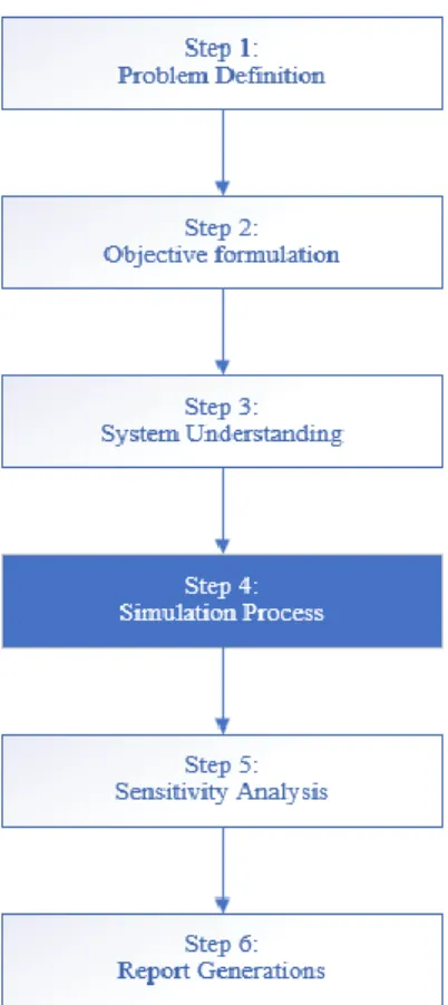
Simulation is not only about replicating a real-world scenario, it is also the best representation of the system and their complex interrelationships as a function of time (Rossetti, 2015). The idea is that the required future system is achieved by a flexible model of the real physical system, coupled with its correlated elements, modelled and validated with various scenarios until the predicted system is obtained. The process flow shown in Figure 8 is adopted to meet the problem’s objective.
22
In order to simulate, the foremost step is to understand the problem and identify the scope. In this chapter, sections 1.2 and section 1.3 explain these steps 1 and 2 of the simulation process. Step 3 is dedicated to system understanding, and formulating the model decisions which support in ensuring that the simulation model is able to address the problem for a system considered. Section 3.1 and section 3.2 gives a more elaborate description with respect to the decisions, assumptions etc. Step 4 is the simulation process. This is an iterative process which is further clarified in Figure. 9. The flow defines on how the model is developed. It comprises of four stages: Model Conceptualization, Numerical Analysis, Model Implementation and Model Execution.
Model Conceptualization
Before the model implementation, a UML design is formulated with the system definitions set with respect to the inputs and outputs that require to be considered. A case diagram is first formulated to understand on the flow between the supply chain members namely consumers, retailers, and warehouse. By drawing the case diagrams, the activity flow in the system is clarified and this is reviewed against the essentials that are necessary towards the defined problem. Section 3.2 describes the representation of the flow with respect to the three scenarios under discussion.
Numerical Analysis
To evaluate the conceptualized model theoretically, a numerical analysis is carried out. An excel based macro sheet (Rossetti, 2015) has been adapted and updated to be used for various set of values to understand on the total cost of the supply chain with respect to the three levels of
23
considered collaboration. Three excel spreadsheets are implemented based on the three level scenarios and mathematically the values are generated so that the model results could be validated according to it. Appendix A gives the view of the three spread sheet which has the mathematical evolution carried out before the model execution.
Model Implementation
With the model concept and the numerical analysis sheet, the adaption of the real system to the Arena simulation model is carried out. The level of detailing is ensured to be as close to the concept planned and for the inputs as designed from the numerical analysis sheet. Before the model is implemented in the Arena, the variables, attributes, events and queues are first identified with respect to both the retailer and the warehouse side. These parameters are derived based on the logic that is required to be modeled as detailed in the model conceptualization phase.
Model Execution
The developed model is then run for various demand values to understand on total cost with respect to the collaboration. The model goes through the verification and validation process.
Model Verification
This process is to ensure that the model is complete in all intended aspects and the outputs generated from it is close to the results generated from the numerical analysis sheet. The two main steps followed in this process are the setting up of the initial values and then observing the output
24
for any variations. The main objective of this step would be that if the inputs are set as required then whether the logical structure planned is well represented by the model. This is evaluated from the statistical outputs generated by the model which aids in verifying the model. The input controls are then varied in such a way that all scenarios are covered, also the best and worst scenarios are passed.
Model Validation
This process is carried out to ensure closeness of the model to the real system. In the model validation phase, a Sensitivity Analysis of the system is carried out. The retail world is considered here, hence the parameters and entity set are brought close to the retail environment. The respective controls are identified, and these are varied and the outputs from it are observed. Many trials are executed via the process analyzer tool and the output is studied in relation to the actual system under discussion.
25
3.2 Inventory Level and Cost Calculations
The below notation shall be considered to understand the various cost calculations in the supply chain. Sections 2.4.3, 2.4.4 and 2.4.5 shall be referring to these notations
D – Demand rate per year
LT – Replenishment lead time in days
θ – Poisson distributed Mean demand during replenishment lead time p(x) – Probability mass function
p(x) = 𝜃𝑥𝑒−𝜃
𝑥! x = 0,1,2… G(x) – Cumulative distribution function
G(x) = ∑𝑥𝑖=0𝑝(𝑖) x = 0,1,2…
Q – Reorder Quantity (in units) r – Reorder Level (in units) h – Annual holding cost ($) b – Annual backorder cost ($) o – Annual ordering cost ($)
I(r) – Average inventory on hand with respect to the reorder level r (in units) IN(r) – Net inventory on hand (in units)
26
F(Q,r) – Order frequency with respect to Q and r (in units) S(Q,r) – Fill rate with respect to Q and r (in units)
B(Q,r) – Average backorder number (in units) with respect to Q and r (in units) I(Q,r) – Average On-Hand Inventory (in units) with respect to Q and r (in units)
3.2.1 Demand rate and Lead Time
In inventory management, the two main sources from where uncertainty arises is from the demand rate and the lead time. They are also a key factor in the decision-making process towards which type of inventory policy to consider.
Demand rate could be deterministic or stochastic. Deterministic demand is known in advance and it is certain on what would be the quantity or when it would arrive.
Lead time is the time interval between the placement of order and receipt of the placed order by the customer. Again, lead time here could be constant or varied. Usually lead time has a strong dependence on the supplier.
Demand could follow many different types of distributions but two of the most important distributions available are the (discrete) Poisson Distribution and the (continuous) Normal
Distribution. In Poisson distribution the mean time between the arrival rate λ is exponentially
distributed, so the exponential distribution is f(x) = λ𝑒−λ t λ > = 0.
Also, θ = λ LT
365 which is the expected demand during the lead time. Probability mass function
27 g(x;t) = 𝜃𝑥𝑒−𝜃
𝑥! x = 0,1,2…
(1)
Cumulative distribution function
G(x;t) = ∑𝑥𝑖=0g(x; t) x = 0,1,2… (2)
The frameworks in this chapter consider a stochastic discrete demand which follows a Poisson Distribution and a fixed lead time.
Inventory Theory base formula:
(Zipkin, 2000) has analyzed the (r,Q) inventory model and has resulted in base equations when the demand rate is in a Poisson distribution. The analytical inventory formulas as provided by (Zipkin, 2000) are as below:
Poisson complementary cumulative distribution function:
G0(x;t) = 1 - G(x;t) (3)
Poisson first-order loss function:
G1(x;t) = - (x - λ t) G0 (x;t) + (λ t ) g(x;t) (4) Poisson second-order loss function:
28
3.2.2 Inventory Policy
With the demand being uncertain and random, there are two significant models which could be suited. If in a scenario, random demand occurs the model in which inventory is replenished one unit at a time, then the only issue is to determine the reorder point. The target inventory level set for the system is known as a base stock level, and hence the resulting model is termed the base stock model (Hopp and Spearman, 2011). The model in which the demand occurs randomly, possibly in batches, then here the inventory is monitored continuously. As per (Hopp and Spearman, 2011) when the inventory level reaches (or goes below) r, an order of size Q is placed. After a lead time of l, during which a stockout might occur, the order is received. The problem is to determine appropriate values of Q and r. The model we use to address this problem is known as the (Q, r) model (Hopp and Spearman, 2011). This thesis shall deal more with the (Q,r) model as the policy considered by the retailer and the warehouse follows this policy for satisfying the demand received from the customer.
(Q, r) inventory control policy:
This inventory policy is a continuous review with backordering involved in it. The customer order information keeps coming in one at a time in some stochastic manner. To meet the demand as it arrives the order request is checked against the current stock availability in the system. If it is available, the customer order is relinquished immediately, and the stock availability is decreased by a count. But if stock is not available then the customer order is backordered in a queue which acts on a first come first serve basis. The inventory position is checked every time when ever an order is met or backordered against the reorder point r to decided whether an order needs to be placed. If the inventory position goes below the reorder level r, then a re-order quantity of Q units is placed. This Q units ordered comes after a fixed time, which is the lead time LT from the
29
supplier. After this time once the order is received the customer order as well the backorder as per the queue is met.
Figure 10: (Q,r) inventory model with Q=4 and r=4 (Source: Hopp and Spearman, 2011)
In this concept, there are three main inventory levels and a service rate to understand on. These terminologies are explained as follows
Net Inventory:
This is the inventory on hand or the available stock at a unit of time without considering on the backorder. This inventory keeps decrementing every time a customer order is met and increments whenever a requested order is received. The net inventory is therefore understood as below: Net Inventory = inventory on hand – backorder level
Inventory Position:
This represents the level of net inventory along with inventory in order. On a inventory level it is the actual position at that instant. It is represented as:
30
Since it has all the required inventory level interlinked, it becomes the ideal parameter to check against the reorder level to take a decision on whether to reorder or not.
Backorder Level:
It is the number of units which are backordered as the inventory on hand is not available. It keeps incrementing till the order placed is replenished. It has an associated cost which is charged per unit time till it gets to serve the cost who is waiting on his backordered unit.
Fill rate:
The term fill rate is associated to the stock out condition of the inventory. Stock out represents the duration of time that the system is in the out of stock situation. It is represented in terms of percentage and ideally the lesser the percentage the better is the performance of the system. Fill rate is just 1 minus of the stock out rate. It is the duration for which there is inventory on hand to serve the customer.
Fill rate - 1 – stock out
The average fill rate, backorder level and the inventory level in terms of Q and r has been deduced by (Zipkin, 2000) and it is given as below:
S(Q,r) – Fill rate with respect to Q and r (in units) SO
̅̅̅̅=1 Q [G
1(r ; L) - G1(r+Q ; L)] (6)
B(Q,r) – Average backorder number (in units) with respect to Q and r (in units) B
̅ = 1 𝑄 [G
2(r ; L) - G2(r+Q ;L)] (7)
I(Q,r) – Average On-Hand Inventory (in units) with respect to Q and r (in units)
31
Based on (Zipkin, 2000) equations from (3) to (8), (Hopp and Spearman, 2011) derived the equations for the fill rate, average backorder level and on-hand inventory in terms of the backorder. These equations aid in bringing up an excel based inventory analysis sheet which has been extensively used in the numerical evaluation of the model. The base of the excel has been considered from (Rossetti, 2015) but the formula clarifications are discussed in this section.
S(Q,r) – Fill rate with respect to Q and r (in units) S (Q, r) = 1 - 1
Q[ B(r) – B(r + Q )] (9)
B(Q,r) – Average backorder number (in units) with respect to Q and r (in units) B (Q, r) = 1
Q∑ B(r)
r+Q
r+1 (10)
I(Q,r) – Average On-Hand Inventory (in units) with respect to Q and r (in units) I (Q, r) = Q+1
2 + r –θ + B (Q, r) (11)
3.2.3 Inventory Costs
Some of the financial parameters dealt in the thesis in order demonstrate on the total cost reduction is as described below:
Ordering Cost or Fixed Setup Cost (OC):
This cost is also referred as the replenishment cost and this cost is incurred every time an order is placed. It is the product of number of replenishment /Order Frequency carried out in a year and the replenishment cost factor associated to it. The order frequency as per (Hopp and Spearman,
32
2011) is the number of orders carried out over a period. In thesis the period of consideration is for a year. Hence the order frequency and the associated ordering cost is as per equation given below by the authors
Order Frequency F (Q, r) = D
Q (12)
Ordering Cost (OC) = F(Q,r) * o (13)
Holding Cost (HC):
All the cost that goes into storing of the inventory at a storage location is called the holding cost. It is usually the product of the actual inventory level held and the holding cost factor.
Holding Cost (HC) = I (Q, r) * h (14)
Backorder Cost (BC):
The cost that is incurred every time when ever a customer order is not satisfied is called the Backorder Cost. It is the product of the backorder inventory level and the cost factor associated with the backorder. This cost factor in fact is a penalizing fee on not satisfying the requested customer demand.
Backorder Cost (BC) = B (Q, r) * b (15)
Total Cost (TC):
The sum of all the above costs is the total cost. The total cost of the supply chain needs to be at the minimum so that profit could be improved. The information sharing model considers this total cost to be the performance measure component to understand on how the level of collaboration improves on the reduction of this total cost. This cost considers the ordering cost, holding cost and the backorder cost and its equation is given as below:
33
Total Cost (TC) = OC + HC + BC (16)
3.2.4 Sample (r,Q) Inventory policy Calculation
In order to summarize on the equation’s usage in this thesis, a sample numerical calculation is demonstrated below. This explains on the excel spreadsheets numerical values got for an input control parameter.
Say the annual demand poisson rate D = 50, Lead Time LT = 45 days and the Optimum Controls are Q = 7 and r = 8. Also, for a cost say h = 30$, b = 100$ and 0 = 15$
For equations (9) to (11) the value of p(R), G(r) and B(r) is required, from the excel macros we understand these values and they are as represented in table 4 which represents the fill rate for values of the reorder point.
Table 4: Fill rate for respective R values
So, calculation of the fill rate, Backorder level, Inventory on hand and Order frequency with respect to the function of Q and r are as explained below:
34 S (Q, r) = 1 - 1 Q[ B(r) – B (r + Q)] = 1 - 1 7[ B (8) – B (15)] = 0.949 B (Q, r) = 1 Q∑ B(r) r+Q r+1 = 1 7∑ B(r) r=15 r=9 = 0.0502 I (Q, r) = Q+1 2 + r –θ + B (Q, r) = 7+1 2 + 8 – 6.1644 + 0.050 = 5.886 F (Q, r) = D Q = 50 7 = 7.143
Ordering Cost (OC) = F(Q,r) * o = 7.143 * 15 = 107.145 $ Holding Cost (HC) = I (Q, r) * h = 5.886 * 30 = 176.576 $ Backorder Cost (BC) = B (Q, r) * b = 0.0502 *100 = 5.02 $
Total Cost (TC) = OC + HC + BC = 107.145 + 176.576 $ + 5.02 = 288.741 $
The above calculated inventory levels and costs when compared with the calculations in the excel macros are to be the same. Figure 11 shows the value as seen in the excel spreadsheet which is used by the thesis for the information sharing model.
Figure 11: Inventory level and Cost Calculation Example.
3.3 Supply Chain Collaboration - Model Conceptualization
Three simulation models are developed as per the information level sharing. The models developed align as per the below key assumptions:
35
• The demand follows the Poisson Distribution process • Demand that is not met is backordered
• Replenishment lead time is fixed
According to the levels of information sharing, the partnership collaboration for the three scenarios are as explained below:
3.3.1 No Information Sharing (NIS)
In this case, there is no information sharing between the retailer and the warehouse and order coordination is missing as well. Both the supply members work independently in a more
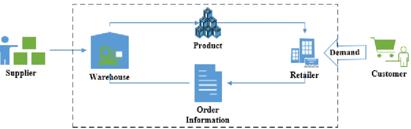
‘decentralized’ manner. This system is more aligned to the traditional supply chain system and the decision making on demand is found to be self reliant. Figure 12 depicts the No Information case. Here, the customer demand arrives to the retailer and based on this information and his on-hand availability of the stock the retailer raises order information to the warehouse. The warehouse similarly based on his available stocks, immediately responds to serve the retailer or raises purchase request with his suppliers, replenishes his stock and then further replenishes the
supplier’s inventory. Figure 12 depicts the flow in which the simulation model is developed. A two-stage network system which includes the retailer and warehouse internally and the customer or supplier at the external end is considered.
36
Figure 12: No Information Sharing (NIS)
The detailed flow of the concept is as per Figure 13. The concept is evolved from the model developed by (Tee & Rossetti, 2003). The authors have considered a warehouse and n retailers in a two-echelon inventory system and simulated it to study the effectiveness of simulation models. Their order flow is as shown in Figure 13. The authors have considered n retailers and the demand processing is as per the compound Poisson demand. The concept of the two-level system is adapted from this work but the thesis is limited to a single retailer and warehouse and hence a poisson demand rate.
37
Figure 13 shows the swim lane diagram to explain on the order flow between the customer, retailer and the warehouse. As the flow indicates, the customer first arrives and places his order. On this request arrival at the retailer side, the retailer processes it as per the (r,Q) policy. If retailer finds that the available inventory is not sufficient, he raises an order with the warehouse. If not, retailer would satisfy the request raised by the customer. The warehouse waits for order request from the retailer and similar to the retailer operates on the (r,Q) policy and replenishes the retailer with either inventory on hand or by replenishment from the supplier.
The performance level of the total cost of both the retailer and warehouse is considered as the prime entity for the information sharing purpose. As seen, there is no coordination here, because as the order arrives the retailer and warehouse work independently with respect to their inventory and serve the upper levels. The fill/service rate of the retailer is more significant as it is the lowest level in the system and it needs to be the highest level.
38
Figure 14: No Information Sharing (NIS) – Swimlane Diagram
(Hopp and Spearman, 2011) have described on how to approach a two-stage system which has a retailer and warehouse operating in continuous inventory policy with constant lead time. This concept has also been adapted in the model. According to the authors the first step would be to
39
place the retailer re-order level and order quantity to 1 so that the warehouse receives the same poisson demand rate as the retailer. This enables us to analyze the warehouse as a single level and fix its optimum values. The backorder level of the warehouse is also known from this analysis. The author describes that the next step is finding the retailers lead time based on the warehouse delivery which is computed by the equation (17) and (18). These equations are provided by (Hopp and Spearman, 2011) and equation (17) is the wait time of an order at the warehouse and equation (18) mean effective lead time at the retailer. In the thesis, the delivery/transport time is kept constant at 1 day.
W = 365∗𝐵 (𝑄.𝑟) 𝐷
(17)
E[L] = Delivery time + W (18)
3.3.2 Partial Information Sharing (PIS)
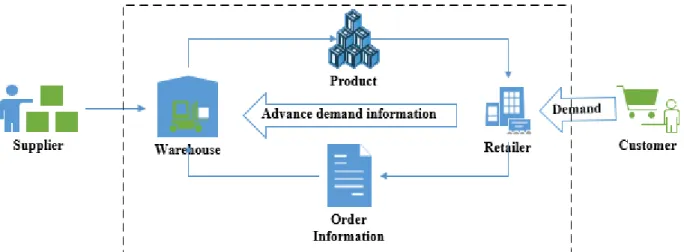
In this case the system is to a certain extent coordinated between the retailer and warehouse. In this level the customer in advance informs the retailer that he would be placing order at a particular duration and also informs on the demand that would be placed and the due date on when he requires it. This information is shared by the retailer to the warehouse and the warehouse also keeps his supplier informed accordingly in order to meet the demand which is expected to arrive. Owing to a certain level of collaboration, the retailer and the warehouse is aware of the information in advance, they get the benefit to plan ahead and ensure to meet the customer demand. This basically leads to the reduction of the lead time which ultimately results in the backorder reduction which
40
translates to cost savings in terms of the total operational costs of the system and profit gain. Figure 15 gives us a representation of the information and material flow in the partial information system.
Figure 15: Partial Information Sharing (PIS)
The PIS system follows the concept explained by (Hariharan & Zipkin, 1995) on processing advance information from customer. The authors have analyzed the benefit of the ADI concept which is about knowing in advance on when a customer would arrive and after what time the customer expect to receive the order. Also, the customers will not receive the order in advance. It needs to be as per the due date set by them. From a conventional system point of view the demand lead time is the time at which the demand/order is placed by the customer. The authors have found that when the supply lead time deteriorates the performance of a system, parameter like the demand lead time elevates it.
From this concept the partial information logic is designed and it is explained in two cases as shown in Figure 16 and Figure 17. Say, 𝐿𝑠 is the supply lead time and 𝐿𝐷 the demand lead time, then there could be two main scenarios. In both scenarios, the customer and the retailer have advance discussion on the order requests. For the early information discussion, the customer brings
41
information on the order quantity and on when he expects the order. The retailer brings his information on the supplier lead time to the discussion.
Case 0: When order delivery time > 𝐿𝑠. In this case the system has no issues and it can work as normal system, and have the order request processed in time and serve the customer on his expected due date. This is an ideal case which rarely occurs. Here the retailer based on the advance information received he could delay the order to his supplier so that the supply lead time aligns to the deliver date of the customer
Figure 16 : Case 0: Order delivery time > Ls
Case 1: When the order delivery time is a value between and 0 and supply lead time 𝐿𝑠. This is a case where the supply lead time may need to be brought forward with the advance arrival information from the customer. So, if a system is aware of 𝐿𝐷 and 𝐿𝑠 then the supply lead time is solved by the authors as L = 𝐿𝑠 − 𝐿𝐷. Here, when the advance info is discussed based on the Ls and order deliver time required by the customer the order arrival from the customer is planned by
42
both the parties. Thus, with preparedness this new lead time information is considered in the system, although it is lesser than the initial value.
Figure 17 : Case 1: 0 < Order Delivery Time < Ls
The PIS system has adapted this concept and has model aligned to it. The reduction in lead time has eventually resulted in backorder reduction which has improved the performance of the total cost.
43
44
3.3.3 Full Information Sharing (FIS)
In this case, the two-stage inventory system reduces to a single stage inventory system. The retailer does not hold any inventory and transfers all demand processing information to the warehouse. As depicted in Figure 19, the retailer gets the demand from the customer and making use of the technology at hand, it updates immediately on the inventory information’s to it. EDI (Electronic Data Exchange comes to play here. The warehouse similarly pulls up the information process’s
the request and supplies the product back to the retailer which is to be directly served to the customer. This is a Full information Sharing concept adapted from the Vendor Managed Inventory system, where in the vendor takes full control of the demand information.
Figure 19 : Full Information Sharing (FIS)
As shown in Figure 20 the retailer publishes the inventory data received from the customer and the warehouse pulls the necessary information required for its processing and process the order and provides the information back to the retailer who in turn supplies the customer. As the upstream members take control of the inventory processing it is more a VMI aligned model.
45
46
4
CHAPTER 4:
DES MODEL TRANSLATION IN ARENA
The concepts detailed in the previous chapter are translated into the Arena models for execution. The DES elements are discussed and then the base simulation concept of the (r, Q) inventory policy for information sharing is explained further on to its translation to Arena model. Figure 21 presents the Arena and the Process Analyzer tool associated with the thesis. Any figure or discussion with respect to the Arena tool in this document will be as per this version and revision.
Figure 21 : Arena Version 15.00.00001
4.1 Elements of the Simulation Model
Computer simulation is found to be very beneficial in simulating the mathematical model. It could be executed many times to check the model reliability. The visualization which comes with it gives the additional advantage. Arena is a software for discrete event simulation based on SIMAN processing language. The thesis uses Arena to run experiments on a test supply chain system. It has many terminologies which define the behaviour of the system being modelled, the system description is clarified below followed by its components to support in better understanding and analysis of the system. Also, terms which are part of the Arena software are detailed for more clarity.
47
4.1.1 System:
It is a set of objects grouped together for some interactions or interdependent coordination between them so that a common objective is achieved by these objects in unison together. In order to model a system, it is critical to understand the concepts behind a system and on the system boundary. The system includes components such as the entities, variables and attributes which work towards the objective being set. For the current issues, the system under discussion is the two stage supply chain system working as per the inventory policy (r,Q). Some of the notable components of the supply chain system would be the retailer and warehouse and their processing of the order which gets raised by the consumer.
4.1.1.1 New Simulation Creation
Following are the steps followed to create a new project in the Arena Software
• In the Arena Software clicking on the main menu ‘File’ and then ‘New’ would be
generating a new Simulation Model.
• Once a new simulation page is available, clicking on ‘Run’ and ‘Setup’ under it leads us to
the Project Parameter page where the project title and other options as Figure is provided. • The required statistics that needs to be collected are required to be chosen in this tab.