228
ISSN 1518-3548
Forecasting Brazilian Inflation Using a Large Data Set
Francisco Marcos Rodrigues Figueiredo
December, 2010
ISSN 1518-3548 CGC 00.038.166/0001-05
Working Paper Series
Edited by Research Department (Depep) – E-mail: [email protected] Editor: Benjamin Miranda Tabak – E-mail: [email protected] Editorial Assistant: Jane Sofia Moita – E-mail: [email protected]
Head of Research Department: Adriana Soares Sales – E-mail: [email protected] The Banco Central do Brasil Working Papers are all evaluated in double blind referee process. Reproduction is permitted only if source is stated as follows: Working Paper n. 228.
Authorized by Carlos Hamilton Vasconcelos Araújo, Deputy Governor for Economic Policy.
General Control of Publications
Banco Central do Brasil Secre/Surel/Cogiv
SBS – Quadra 3 – Bloco B – Edifício-Sede – 1º andar Caixa Postal 8.670
70074-900 Brasília – DF – Brazil
Phones: +55 (61) 3414-3710 and 3414-3565 Fax: +55 (61) 3414-3626
E-mail: [email protected]
The views expressed in this work are those of the authors and do not necessarily reflect those of the Banco Central or its members.
Although these Working Papers often represent preliminary work, citation of source is required when used or reproduced.
As opiniões expressas neste trabalho são exclusivamente do(s) autor(es) e não refletem, necessariamente, a visão do Banco Central do Brasil.
Ainda que este artigo represente trabalho preliminar, é requerida a citação da fonte, mesmo quando reproduzido parcialmente.
Consumer Complaints and Public Enquiries Center
Banco Central do Brasil Secre/Surel/Diate
SBS – Quadra 3 – Bloco B – Edifício-Sede – 2º subsolo 70074-900 Brasília – DF – Brazil
Fax: +55 (61) 3414-2553
Forecasting Brazilian Inflation Using a Large Data Set*
Francisco Marcos Rodrigues Figueiredo**
Abstract
The Working Papers should not be reported as representing the views of the Banco Central do Brasil. The views expressed in the papers are those of the author(s) and
do not necessarily reflect those of the Banco Central do Brasil.
The objective of this paper is to verify if exploiting the large data set available to the Central Bank of Brazil, makes it possible to obtain forecast models that are serious competitors to models typically used by the monetary authorities for forecasting inflation. Some empirical issues such as the optimal number of variables to extract the factors are also addressed. I find that the best performance of the data rich models is usually for 6-step-ahead forecasts. Furthermore, the factor model with targeted predictors presents the best results among other data-rich approaches, whereas PLS forecasts show a relative poor performance.
Keywords: Forecasting inflation, principal components, targeted predictors,
partial least squares.
JEL Classification: C33, C53, F47
*
The author would like to thank Simon Price and José Pulido for their useful comments. I also thank participants at the XII Annual Inflation Targeting Seminar of Banco Central do Brasil and XV Meeting of theCentral Bank Researchers Network of the Americas. The views expressed in this paper are those of the author and do not necessarily reflect those of the Banco Central do Brasil.
**
"Prediction is very difficult, especially if it's about the future." Nils Bohr, Nobel laureate in Physics
1 - Introduction
Forecasting inflation is a critical issue for conducting monetary policy regardless of whether or not the central bank has adopted a formal inflation targeting system. Since there are transmission lags in the impact of monetary policy in the economy, changes in the monetary policy should be based on projections of the future inflation. Therefore, the prime objective of inflation forecasting in a Central Bank is to serve as a policy tool for the monetary policy decision-making body.
Saving, spending and investment decisions of individual households, firms and levels of government, both domestic and foreign, affect the aggregate price level of a specific country. Therefore, the determinants of inflation are numerous and include variables such as monetary aggregates, exchange rates, capacity utilization, interest rates, etc. Central banks in general and the Brazilian central bank (BCB) in particular keep an eye on a very huge set of variables, including those that are likely to affect
inflation. The BCB, for example, provides electronic access1 to economic databases
included in the Economic Indicators (Indicadores Econômicos). The data are broken up into six categories: economic outlook that includes price, economic activity, sales, etc.; currency and credit; financial and capital markets; public finance; balance of payments; and international economy. It constitutes a very comprehensive description of the Brazilian economy and is currently available to the monetary authorities. Additionally, the Brazilian central bank assesses the state of the economy each quarter and has published forecasts for inflation and GDP in its Inflation Report since 1999.
Despite central bank monitoring of a very large number, even thousands, of those economic variables that possibly affect inflation, the most common methods employed for forecasting inflation, such as Phillips curve models and vector autoregressions, customarily include only few predictors. Nonetheless, recent methodologies have been developed and employed in order to take advantage of large datasets and computation capabilities available nowadays. Stock and Watson (2006) describe different approaches for forecasting in a data-rich context.
1
It is common to identify two broad approaches for forecasting in a data-rich environment: (a) one can try to reduce the dimensionality of the problem by extracting the relevant information from the initial datasets and, then use the resulting factors for forecasting the variable of interest. Factor models with their different techniques and partial least squares (PLS) are examples of this first approach; and (b) one can just try to pick the relevant information from the individual forecasts provided by numerous models that usually do not contain more than few variables for each model. Classical forecast combination, Bayesian model averaging (BMA) and bootstrapping aggregation (Bagging) represent this approach for forecasting in a data rich environment.
The objective of this paper is to verify if exploiting the large data set available to the Central Bank of Brazil makes it possible to obtain forecast models that are serious competitor to models typically used by the monetary authorities for forecasting inflation. Incidentally, some empirical issues such as the optimal number of variables to extract the factors are also addressed.
I focus on two data-rich techniques for macroeconomic forecasting. First, I discuss the factor modeling by principal components (PC) developed by Stock and Watson (1998) and then I estimate a few underlying factors from a large dataset for the Brazilian economy and then employ the factors to forecast monthly inflation. I also provide a model using PC factors obtained from a reduction dataset in the spirit of the targeted predictors by Bai and Ng (2008). The second method is partial least squares (PLS), in which the extracted factors depend on the variable to be forecasted. The predictive performances of the proposed models and models similar to those used by the central banks are assessed through “quasi” pseudo out-of-sample simulation exercises.
I find that the best performance of the data rich models is usually for 6-step-ahead forecasts and forecasting models using rolling regressions outperform models based on recursive estimations. Furthermore, the factor model with targeted predictors presents the best results among the other data-rich approaches whereas PLS forecasts show a relative poor performance.
This paper is organized as follows. Next section presents a brief discussion about the models usually used for forecasting inflation putting emphasis on those customarily used by monetary authorities. The following two sections (sections 3 and 4) describe two suitable forecasting methods to be used with a large number of predictors: the factor models by principal components and partial least squares. I also discuss some empirical issues concerning the extraction of the factors such as the number of factor and the
“optimal” size of the dataset. In section 5, the forecasting framework is set up and I briefly describe some models used by the Central Bank of Brazil for forecasting inflation. Empirical results are presented in section 6. Finally, I offer some concluding remarks and suggest some extensions for future research.
2 - Models for forecasting inflation
Macroeconomic forecast has been improved through time in the last fifty years. From macro models following the tradition of Cowles Commission to the Box-Jenkins approach represented by ARIMA models and their offspring, the econometric modeling has been given more attention to the data generating process underlying the economic time series.
One of the most traditional ways to predict inflation is by using models based on short-run Phillips curve, which says that short-term movements in inflation and unemployment tend to go in opposite directions. When unemployment is below its equilibrium rate, indicating a tight labor market, inflation is expected to rise. On the other hand, when unemployment is above its equilibrium rate, indicating a loose labor market, inflation is expected to fall. The equilibrium unemployment rate is often referred to as the Non-Accelerating Inflation Rate of Unemployment (NAIRU). The modern version of the Phillips curve used to forecast inflation is known as NAIRU Phillips curve. Atkeson and Ohanian (2001) observe that NAIRU Phillips curves have been widely used to produce inflation forecasts, both in the academic literature on inflation forecasting and in policy-making institutions.
However, several authors have largely challenged this practice. Atkeson and Ohanian (2001) challenge the usefulness of the short-run Phillips curve as a tool for forecasting inflation. According to them and Stock and Watson (1999), Phillips curve based forecasts present larger forecast errors than simple random walk forecasts of inflation. On the other hand, Fisher, Liu, Zhou (2002) show that the Phillips curve model seems to perform poorly typically when a regime shift has recently occurred, but even in this case, there may be some direction information in these forecasts that can be used to improve naive forecasts. Likewise, Lansing (2002) claims the evidence suggests that the short-run Phillips curve is more likely to be useful for forecasting the direction of change of future inflation rather than predicting actual magnitude of future inflation.
Some other methods for forecasting inflation are more related to a data-driven framework. Some authors, for example, have been searching for an individual indicator
or variable that would be able to provide consistent forecasts of inflation. But the results have been fruitless as it can be seen in Cecchetti, Chu and Steindel (2000), Chan, Stock and Watson (1999), Stock and Watson (2002a) and Kozicki (2001). The basic message of the studies is that there is no single indicator that clearly and consistently predicts inflation. Nonetheless, Cecchetti, Chu and Steindel (2000) assert that a combination of several indicators might be useful for forecasting inflation.
Among the data-driven models, the vector autoregression (VAR) approach, due to Sims (1980), became an effective alternative to the large macroeconomic models of the 1970s and it has also gained a great appeal in terms of forecast inflation. The VAR model, in its unrestricted version, is a dynamic system of equations that examines the linear relationships between each variable and its own lagged values and the lags of all other variables without theoretical restrictions. The only restrictions imposed are the choice of the set of variables and the maximum number of lags. The number of lags is usually obtained from information criteria such as Akaike or Schwarz. The VAR approach supposes that all variables included in the model are stationary. An alternative process to handle non-stationary variables is the vector error correction (VEC) model.
The popularity of VAR methodology is in great part due to the lack of need of a hypothesis for the behavior of the “exogenous” variables to forecast. The model not only has a dynamic forecast of the variables, but also presents a great capacity to short-term forecasting. The relative forecast performance of the VAR model has made it a part of the toolkit of central banks.
Even so, the VAR methodology presents some shortcomings. One limitation of these models is the over-parameterization, which reduces degrees of freedom, increasing the confidence intervals. Another problem is the large prediction errors generated by the dynamic processes of the model.
In order to solve, or at least reduce the problems mentioned above, incorporating previous researcher knowledge about the model originates the Bayesian VAR (BVAR), methodology.
Basically, Bayesian VAR approach uses prior statistical and economic knowledge for guessing initial values for each one of the coefficients. The prior distribution is then combined with the sample information to generate estimates. The prior distribution should be chosen so as to provide a large range of uncertainty, and to be modified by the sample distribution if both distributions differ significantly.
Currently, different versions of vector autoregression models are largely employed for forecasting inflation in central banks such as the Federal Reserve Bank and Bank of England. A brief description of some VAR models used in the Brazilian central bank is presented in Section 3.
Nevertheless, one common characteristic of all models discussed above is that they only include few variables as explanatory variables and consequently they do not exploit the whole information available to central banks, which comprises hundreds to thousands of economic variables.
Some authors claim that including more information in the models lead to better forecasting results. Stock and Watson (1999), for example, show that the best model for forecasting inflation in their analysis is a Phillips curve that uses, rather than a specific variable, a composite index of aggregate activity comprising 61 individual activity measures.
In order to take advantage of very large time series datasets currently available, some recent and other not so recent methodologies have been suggested. Stock and Watson (2006) survey the theoretical and empirical research on methods for forecasting economic time series variables using many predictors, where "many" means hundreds or even thousands. One important aspect that has made possible the advancements in this area is the improvements in computing and electronic data availability in the last twenty years.
Combination of forecasts of different models represents one possible way to use the rich data environment. This approach has been used in economic models for forty years since the seminal paper of Bates and Granger (1969). Newbold and Harvey (2002) and Timmermann (2006) are examples of more recent survey articles on this subject. Stock and Watson (2006) provide a discussion on forecast combination methods using a very large number of models.
Among the more recent methodologies discussed by Stock and Watson (2006), some of them deserve special attention since they have been applied extensively in economics lately, such as the factor model analysis; they either represent generalization or refinement of other methods such as the partial least square methodology (PLS) and the Bayesian model averaging (BMA). In the next two sections, the methodologies of factor model and PLS are discussed. BMA will hopefully be future subject of my research.
3 - Model for dealing with large dataset: dynamic factor model
As discussed by Stock and Watson (2006), there are several techniques for forecasting using a large number of predictors. Dynamic factor models, ridge regression, Bayesian techniques, partial least squares and combinations of forecasts are examples of possible approaches that have been used in macroeconomic forecasts. In this section, I describe the dynamic factor model, one of the most popular methodologies in this context nowadays that has been largely used in central banks and research institutions as forecasting tools.2
3.1 - Factor analysis and principal component models
The objective of this section is to present the methodology for estimating a few underlying factors using the methodology based on factor models proposed by Stock
and Watson (1998). The factor model3 is a dimension reduction technique introduced in
economics by Sargent and Sims (1977). The basic idea is to combine the information of a large number of variables into a few representative factors, representing an efficient way of extracting information from a large dataset. The number of variables employed in most applied papers usually varies from one hundred to four hundred, but in some cases the datasets can be larger such as Camacho and Sancho (2003). They use a dataset with more than one thousand series.
Bernanke and Boivin (2003) claim that the factor model offers a framework for analyzing data that is clearly specified, but that remains agnostic about the structure of the economy while employing as much information as possible in the construction of the forecasting exercise. Moreover, since some estimation methods of this type of model are non-parametric such as those based on principal components, they do not face the problem that a growing number of variables lead to an increased number of parameters and higher uncertainty of coefficient estimates as in state-space and regression models. As emphasized by Artis et al. (2005), this methodology also allows the inclusion of data of different vintages, at difference frequencies and different time spans.
Following Sargent and Sims (1977), several papers have employed this method in different areas of economics. For example, Conner and Korajczyk (1988) used this method in arbitrage pricing theory models of financial decision-making. Additionally,
2
A good glimpse of theoretical and applied works on this subject is given by the papers presented at the research forum: New developments in Dynamic Factor Modelling organized by the Centre for Central Banking Studies (CCBS) at Bank of England in October 2007.
3
this methodology has also been employed for obtaining measures of core inflation, indexes for monetary aggregates and for human development.
In terms of macroeconomic analysis, most studies are concerned with monetary policy assessment and evaluation of business cycles (Forni et al. (2000)). Bernanke and Boivin (2003), for instance, introduced the factor-augmented vector autoregressions (FAVAR) to estimate policy reaction functions for the Federal Reserve Board in a data-rich environment.
Gavin and Kliesen (2008) argue that another reason for the popularity of the dynamic factor model is because it provides a framework for doing empirical work that is consistent with the stochastic nature of the dynamic stochastic general equilibrium (DSGE) models. Boivin and Giannoni (2006) and Evans and Marshall (2009) are examples of using dynamic factor framework with the theory from DSGE models to identify structural shocks.
For Brazil, we have very few examples of studies using dynamic factor methodology. Ortega (2005) used factors extracted from 178 time series as instruments in forward-looking Taylor rules and as additional regressors in VARs to analyze monetary policy in Brazil. Ferreira et al. (2005) employed linear and nonlinear diffusion index models to forecast quarterly Brazilian GDP growth rate.
Regarding forecasting of macroeconomic variables, mainly output and inflation, it has been noticed an increasing number of papers in the recent years for different countries. Eickmeier and Ziegler (2008) is one example of recent survey of the literature of dynamic factor models for predicting real economic activity and inflation.
Since the pioneer work of Stock and Watson (1998), Eickmeier and Ziegler (2008) list 47 papers for more than 20 different countries using dynamic factor models. The vast majority of the papers (37) have been written since 2003. Most studies found that the forecasts provided by this methodology have smaller mean-squared errors than forecasts based upon simple auto regressions and more elaborate structural models.
Currently, it seems that the main use of factor models is as forecasting tools in central banks and research institutions. The potential of factor forecasts has been investigated by various institutions including the Federal Reserve of Chicago, the U.S. Treasury, the European Central Bank, the European Commission, and the Center for Economic Policy Research. Some institutions went a step further and have been integrating factor models into the regular forecasting process. The Federal Reserve Bank of Chicago produces a monthly index of economic activity (Chicago Fed National
Activity Index – CFNAI) that is basically the first static principal component from a set of 85 monthly indicators of economic activity in the United States. Another example is the EuroCOIN that is a common component of the euro-area GDP, based on dynamic principal component analysis developed by Altissimo et al. (2001).
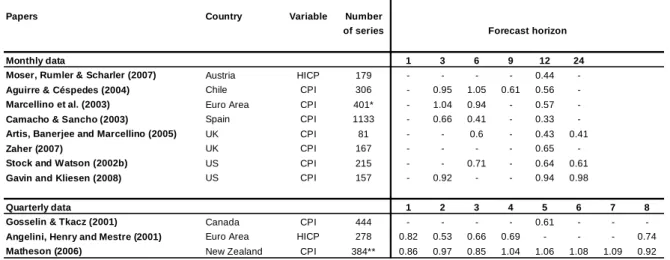
Table 3.1 shows a summary of several studies where factor is employed for
forecasting inflation. The table displays the root mean square forecast error (RMSFE) of factor models relative to the best univariate autoregressive models. Figures lower than one mean that the factor model presents a lower RMSFE than the benchmark model.
The results show that factor models usually outperform the autoregressive model. The average gain for a 12-step ahead forecast for monthly inflation, for example, is close to 40 percent. Furthermore, the relative performance of the factor model in the monthly examples seems to be improved for longer forecasting horizons.
Despite the very promising results of early works, Eickmeier and Ziegler (2008) argue that some studies such as Schumacher (2007), Schumacher and Dreger (2004) find no or only negligible improvements in forecasting accuracy using factor models. This leads to what I consider the second wave of papers in the literature, where the main focus change from comparing the performance of factor models against benchmark forecasts to explore in which context the factor model perform better. Boivin and Ng (2006) and Jacobs et al. (2006) are examples of this literature. They want to verify if the larger the dataset, the better is the forecasting performance of the model as well as how the results depend on the characteristics of the datasets and the factor.
Table 3.1 Summary of factor model results for forecasting inflation: RMSFE relative to autoregressive models
Papers Country Variable Number of series
Monthly data 1 3 6 9 12 24
Moser, Rumler & Scharler (2007) Austria HICP 179 - - - - 0.44
-Aguirre & Céspedes (2004) Chile CPI 306 - 0.95 1.05 0.61 0.56
-Marcellino et al. (2003) Euro Area CPI 401* - 1.04 0.94 - 0.57
-Camacho & Sancho (2003) Spain CPI 1133 - 0.66 0.41 - 0.33
-Artis, Banerjee and Marcellino (2005) UK CPI 81 - - 0.6 - 0.43 0.41
Zaher (2007) UK CPI 167 - - - - 0.65
-Stock and Watson (2002b) US CPI 215 - - 0.71 - 0.64 0.61
Gavin and Kliesen (2008) US CPI 157 - 0.92 - - 0.94 0.98
Quarterly data 1 2 3 4 5 6 7 8
Gosselin & Tkacz (2001) Canada CPI 444 - - - - 0.61 - -
-Angelini, Henry and Mestre (2001) Euro Area HICP 278 0.82 0.53 0.66 0.69 - - - 0.74
Matheson (2006) New Zealand CPI 384** 0.86 0.97 0.85 1.04 1.06 1.08 1.09 0.92
Source: Papers referred above and Eickmeier & Ziegler (2008). * Balanced panel.
** The authors use data reduction rules.
In addition to the size of the dataset and the characteristics of the variables, estimation techniques might play an important role in the factor forecast model. The chosen method might also affect the precision of the factor estimates. Boivin and Ng (2005) asserts that the two leading methods in the literature are the “dynamic” method of Forni et al. (2000, 2005) and the “static” method of Stock and Watson (2002a, b). Boivin and Ng (2005) also show that besides the static method being easier to construct than the dynamic factor, it also presents better results in empirical analysis. In the next subsection I will describe the methodology developed by Stock and Watson (2002a, b).
3.2 - Model specification and estimation
The basic idea of the factor model is that it is possible to reduce the dimension of a large dataset into a group of few factors and retain most of the information contained in the original dataset. In the approximate factor model, each variable is represented as the sum of two mutually orthogonal components: the common component (the factors) and the idiosyncratic component.
Let us denote the number of variables in the sample by N and the sample size by T. In this methodology, the number of observations does not restrict the number of explanatory variables, so N can be larger than T. Assuming that the variables can be represented by an approximate linear dynamic factor structure with q common factors I have:
(3.1) with i = 1, …, N and t = 1, …, N .
Xit represents the observed value of explanatory variable i at time t and ft is the q
x 1 vector of non-observable factors and eit is the idiosyncratic component. The 1 x q
shows how the factors and their lags determine Xit.
There are different estimation techniques for the model defined by (3.1). Besides the approaches proposed by Stock and Watson (SW) (2002a) and Forni, Hallin, Lippi and Reichlin (FHLR) (2005) that rely on static and dynamic principal component
analysis4 respectively, Kapetanios and Marcellino (2004) suggest a method based on
subspace algorithm. As mentioned before, Boivin and Ng (2005) claim that the SW approach presents better results in empirical analysis.
4
Whereas SW methodology is based on the second moment matrix of X, the FHLR method components are extracted using the spectral densities matrices of X at various frequencies.
In order to solve the model by principal components as in Stock and Watson (2002a) I need to make the model static in the parameters. The model in its static representation is the following:
(3.2)
where Xt is the vector of time series at time t and
'
t
F dimension column vector of
stacked factors and Λis the factor loading matrix relating the common factors to the
observed series that is obtained by rearranging the coefficients of λi(L)for i = 1,…, n. Note that F , t Λand εt are not observable.
The goal of principal component analysis is to reduce the dimension of the dataset, whereas keeping as much as possible the variation present in the data. In this context, I have to choose the parameters and factor of the model in (3.2) in order to maximize the explained variance of the original variables for a given number of factors
q ≤ N. The resulting factors are the principal components.
In this context, the principal component analysis is represented by an eigenvalue
problem of the variance-covariance matrix of the time series vector Xt and
the corresponding eigenvectors form the parameter matrixΛand the weights of the
factors Ft.
(3.3) Λ
Λ is obtained by setting it equal to N1/2 times the eigenvectors of the N x N matrix corresponding to its largest q eigenvalues. When N > T, Stock and Watson
(1998) recommend a computationally simpler approach where Fˆis setting equal to T1/2
times the eigenvectors of the T x T matrix XX’ corresponding to its q largest eigenvalues.
As the principal component method is a non-parametric method, it does not suffer the problems that a growing cross-section dimension leads to: an increased number of parameters and higher uncertainty of coefficient estimates, as in state-space models and regression approaches.
An estimated factor can be thought as a weighted average of the series in the dataset, where the weights can be either positive or negative and reflect how correlated each variable is with each factor. Factors are obtained in a sequential way, with the first factor explaining most of the variation in the dataset, the second factor explaining most of the variation not explained by the first factor, and so on.
3.3 - Choosing the number of factors
One key point of this approach is the number of factors to extract from the dataset. The decision of when to stop extracting factors basically depends on when there is only very little “random” variability left. There have been examples in the literature of formal and informal methods of choosing the number of factors.
Some methods are based on the idea that eigenvalues of the sample correlation matrix may indicate the number of common factors. Since the fraction of the total variance explained by q common factors is denoted by:
(3.4) ∑ೖసభ
where is the ith eigenvalue in descending order, it would be possible to choose the
number of factor by a specific amount of the total variance explained by the factors. However, there is no limit for the explained variance that indicates a good fit. Breitung and Eickmeier (2006) notice that in macroeconomics panels, a variance ratio of 40 percent is regularly considered as a reasonable fit.
Matheson (2006), Stock and Watson (1999, 2004), Banerjee et al. (2005, 2006), Artis et al. (2005) set a maximum number of factors and lags simultaneously to be included in the forecasting equation using information criteria. On the other hand, Bruneau et al. (2003) seek to assess the marginal contribution of each of the factors to the forecast. Schumacher (2007), Forni et al. (2000, 2003) use performance-based measures, mean squared error, for example.
In most of the applied papers in economics, such as Angelini et al. (2001) and Camacho and Sancho (2003), the decision is based on the forecast performance. Nonetheless, Bai and Ng (2002) have proposed ways to determine the number of factors
based on information criteria using the residual sum of squares given by Equation 3.55 plus a penalty term that is an increasing function of N and T.
(3.5) ,
∑ ∑ ′
The two criteria which performed better in the authors’ simulations are the following: (3.6) ln, !" (3.7) ln, !"min &, '(
The first term on the right hand side in 3.6 and 3.7 shows the goodness-of-fit that is given by the residual sum of squares, which depends on the estimates of the factors and the numbers of factors. The information criteria above can be thought of as extensions to Bayes and Akaike information criteria.
They display the same asymptotic properties for large N and T, but they can be different for a small sample. In empirical applications, a maximum number of factors
are fixed (rmax) and then estimation is performed for all number of factors (r = 1,2
…rmax). The optimal number of factors minimizes the Bai-Ng information criterion
(BNIC).
Matheson (2006) criticizes Bai and Ng criterion claiming that this approach retains a large number of factors leading to possible problems of degrees of freedom.
3.4 - Data with different frequencies and missing values
The principal component approach and the corresponding matrix decomposition described above are valid in the presence of balanced panel, i.e. datasets in which no data are missing. However, Stock and Watson (1998) demonstrated that it is still possible to perform the estimation in the presence of missing values using the expectation maximization (EM) algorithm. The EM algorithm is a method used to estimate probability densities under missing observation through maximum-likelihood estimates for parametric models. In the first step, the estimated factor from balanced
5
panel can be used to provide estimates for the missing observations. Then factors are obtained from the completed data set and the missing observations are re-estimated using the new set of estimated factors, and the process is iterated until the estimates of the missing observations and of the factors do not change substantially.
This feature allows combining data with different frequencies, for example monthly and quarterly. It also allows incorporating series that are only available for sub periods. The downside of this procedure is the existence of the risk of substantial deterioration of the final factor obtained from the entire dataset. Angelini (2001) observed that the deterioration increases when the number of factors in each EM iteration is large.
In their survey of forecasting applications of dynamic factor models, Eickmeier and Ziegler (2006) find that balanced or unbalanced panels and the specification of forecasting equation seem to be irrelevant for the forecast performance.
3.5 - Choosing the “optimal” data size
How the number of series affects the forecasting performance of factor models is still an open question in the empirical literature. In this part, I discuss some possible problems of using “too many” series as well as the routines suggested by some authors to choose the optimal numbers of series to be included in the forecasting factor model.
In this forecasting framework, forecasts can be considered linear projections of the dependent variable on some information set ):
(3.8) * +,-.*|)
Assuming that f(.) represents the operator for the principal component analysis, then Stock and Watson (2002) forecasts that use the whole available information set is given by:
(3.9) * +,-.*|)
One aspect that is object of current studies in the empirical literature of dynamic factor is the selection of an optimal subset of ). The authors of early studies, as argued
in Matheson (2006), at least tacitly, advocate the use of as many time series as possible to extract the principal components.
The idea behind this statement is that the larger the dataset tends the greater the precision of the factor estimates is. However, intuitively, one can conceive that including not relevant and/or not informative variables might spoil the estimate factors. In effect, Boivin and Ng (2006) demonstrate that increasing N beyond a given number can be harmful and may result in efficiency losses, and extracting factor from larger datasets does not always yield better forecasting performance. However, it is not only the size of the dataset that matters for forecasting, the characteristics of the dataset is also important for the factor estimation and for the forecast performance.
Boivin and Ng (2006) show that the inclusion of variables with errors, which have large variances and/or are cross-correlated, should worsen the precision of factor estimates. One possible problem is oversampling, the situation where the dataset include many variables, which are driven by factors irrelevant to the variable of interest. In this context, a better estimation of the factors does not turn into a better-forecast performance. Other features of the data can also undermine the precision of the factor estimates and the forecasting performance. One is the dispersion of the importance of the common component and other is the amount of cross and serial correlations in the idiosyncratic components.
The authors proposed some kind of pre selection of the variables before the estimation and forecasting stages in order to remove correlated, large errors or irrelevant variables. They suggest excluding those series that are very idiosyncratic and those series with highly cross-correlated error in the factor model. Another possible approach is categorizing the data into subgroups with an economic interpretation.
As the objective is forecasting a specific variable, another approach for reducing the initial dataset should be based on the predictive power of the candidate variables. Bai and Ng (2008) denote as targeted predictors those candidate variables in the initial large dataset which are tested to have predictive power for the variable to be forecasted. Thus I call the PC factor forecasting model obtained from the reduction of the initial dataset based on the prediction ability of the variables as targeted principal component (TPC) model
Some authors have been proposing different ways to ‘target” the variables from which the factor would be extracted. Den Reijer (2005), for example, verifies whether the series lead or lag the time series of forecasting interest, and he shows that for the
whole set of leading components there exists an “optimal”, not necessarily a maximum size of the subset of data, at which the forecasting performance is maximized. Thus, he reduces the information set to ) that comprises all variables that are leading to the dependent variable.
However, Silverstovs and Kholodin (2006) criticize den Reijer (2005) observing that leading time series need not necessarily imply a better forecasting performance and they propose to search for variables, which are individually better at forecasting the variable of interest. As a result, the information selected by Silverstovs and Kholodin
(2006), ), includes only series that have the out-of-sample root mean square
forecast error (RMSFE) lower than that of a benchmark model. They conclude that their procedure yields large improvement in the forecasting ability over the model based on the entire dataset and outperforms the approach suggested by der Reijer (2005).6
Similarly, Matheson (2006) exploits the past predictive performance of the indicators in terms of the relevant dependent variable to vary the size of the data. Formally, he estimated OLS regressions of the forecast on each potential indicator and sorted them out from most to least informative in terms of R2. Then he chose a specific top proportion 0 of the ranked indicators to be part of the relevant dataset ()). An alternative way used by the author is using the common component of each indicator (the projection of each indicator on the factor) resulting from the factor model estimated over the entire data set to be as the regressors of the OLS regressions mentioned above. In this approach, the dataset employed and, consequently, the estimated factors are conditional to the variable of interest and forecast horizons.
However, the results obtained by Matheson are unclear both in terms of finding a relationship between the size of the data set and forecast performance and of which data-reduction rule produces the best factor model forecasts.
Bai and Ng (2008) use two classes of procedures to isolate the subset of targeted variables. In the first procedure which they call as hard thresholding, they estimate regressions of * against each 1 controlling for lags * and then rank the variables by
their marginal predictive power through the t statistic associated with 1. The second
approach called as soft thresholding performs subset selection and shrinkage
6
One feature of the method employed by Silverstovs and Kholodin (2006) is that the information set is dependent on the forecast horizon since the forecasting accuracy and the leading capacity might change for different values of h.
methodology simultaneously using some extensions of ridge regression. They authors found that TPC models perform better than no targeting at all.
The basic message of this section is that noisy data can do harm in the extraction of factors and affect our forecasting results. Therefore, reducing the initial dataset by excluding noisy variables or keeping those more related with the variable to be forecasted would improve the forecasts results.
In the next section, I will briefly discuss the Partial Least Square method which extracts the factors taking into account the variable to be forecasted without reducing the initial dataset.
4 - Model for dealing with large dataset: partial least squares
Lin and Tsay (2005) claim that a drawback of the dynamic factor model in forecasting applications is that the decomposition used to obtain the factors does not use any information of the variable to be forecasted. Thus, the retained factors might not have any prediction power whereas the discarded factors might be useful. A possible solution for this problem is the partial least squares (PLS) method.
PLS is an approach that generalizes and combines features from principal component analysis and multiple regressions. This approach is suitable for applications where the number of predictors is often much greater than the sample size and they are collinear. This method emphasizes the question of predicting the responses and not necessarily on trying to understand the underlying relationship between the variables.
Despite being proposed as econometric technique by Wold (1966), it has become popular among chemical engineers and chemometricians Most of its applications concern spectrometric calibration, monitoring and controlling industrial process. It has since spread to research in education, marketing, and the social sciences. Few examples of the utilization of PLS in forecasting macroeconomic variables are available up to the present time but they have been showing promising preliminary results Lin and Tsay (2006) compares PLS with other techniques for forecasting monthly industrial production index in U.S. using monthly dataset with 142 economic variables. Groen and Kapetanios (2008) apply PLS and principal components along with other methodologies on 104 monthly macroeconomic and financial variables to forecast several macroeconomic series for US. They found that PLS regression was generally the best performing forecasting method, and even in the few cases when it is outperformed by other methods, PLS regression still is a close competitor. Additionally,
Eickmeier and Ng (2009) forecast GDP growth for New Zealand using different data-rich methods and conclude that PLS method performs very well compared to other methods.
The major difference between principal component and partial least square is that principal components are obtained taking into account only the values of the variables to be used as the predictors, whereas in the partial least squares, the relationship between the predictors and the variable to be forecasted is considered for constructing the factors. Groen and Kapetanios (2008) provide theoretical arguments for asymptotic similarity between principal components and PLS method when the underlying data has a factor structure. They also argue that forecast combinations can be considered as a specific form of PLS regression.
PLS method finds components from the predictors that are also relevant for the dependent variable. Specifically, PLS regression searches for a set of components
(latent vectors) that performs a simultaneous decomposition of and * with the
constraint that these components explain as much as possible of the covariance between and *. Then the components is used to predict *.
4.1 - Estimation
As mentioned by Groen and Kapetanios (2008), there are several definitions for partial least squares as well as the corresponding algorithms to compute them. But the concept that underlies the different ways to define PLS is that the PLS factors are those linear combinations of the predictor variables that give maximum covariance between the variable to be forecasted and those linear combinations while being orthogonal to each other. Groen and Kapetanios (2008) presented the following algorithm to construct PLS factors:
1) Set 2 * and 3, 1,, i = 1, … N. Set j = 1;
2) Determine N x 1 vector of loading 4 4 5 4 by
computing individual covariances: 4 6-32, 3, i = 1, … N. Construct the
j-th PLS factor by taking the linear combination given by 4′3 and denote this factor by ,;
3) Regress 2 and 3, , i = 1, … N on ,. Denote the residuals of
4) If j = k stop, else set 2 27,3, 37, i = 1, … N and j = j+1 and go to step 2.
The precise number of extracted factors is usually chosen by some heuristic technique based on the amount of residual variation. Alternatively, some authors construct the PLS model for a given number of factors on one set of data and then to test it on another, choosing the factors of extracted factors for which the total prediction error is minimized.
After computing the PLS factors by the algorithm above I use them to forecast inflation using the model to be described in next section.
5 - Forecasting framework
In this part, I outline the forecast models to be compared in the analysis as well as the metrics to be used for assessing the forecast accuracy and performance of the models. I begin with a general description of the forecast model.
5.1 - The dynamic forecast model
Forecast models are specified and estimated as a linear projection of an h-step-ahead variable (8 ) onto predictors at time t.
(5.1) 8 9 :;8 <;= >
where ? is a scalar lag polynomial, @ is a vector log polynomial, μ is a constant
and Zt is a vector of predictor variables at time t and is an error term.
This approach is known as dynamic estimation (e.g. Clements and Hendry, 1998) and differs from the standard approach of estimating a one-step-ahead model and then iterating the model forward to obtain h-step-ahead predictions. The advantages of the dynamic estimation is that there is no need for additional equations for simultaneously forecasting Zt, and the potential impact of specification error in the
one-step-ahead model can be reduced by using the same horizon for estimation and for forecasting. A particular feature of this approach is that for each h we have a different equation since the dependent variable differs for each forecast horizon.
The characterization of * depends on whether the variables of interest, the
or not. For the results to be presented in section 5, I consider inflation as an I(0) process and the relevant variable for most models is
(5.2) * ln శ
where A is either the broad consumer price index (IPCA) or the market price IPCA.7
5.2 - Forecast models
Principal component (PC) forecasts are based on setting Zt in (5.1) to be the
principal components () from a large number of the candidate predictor time series.
is a k x 1 vector estimated using the method discussed in section 3.2. If I use any
method for reducing the initial set of predictor variables, the resulting factors are
denoted as and they are used in (5.1) to obtain targeted principal components
(TPC) forecasts. Zt can also be formed by factors estimated by the algorithm given in
section 4.1 and the resulting forecasts are denoted as partial least squares (PLS) forecasts. The benchmark forecasts are provided by univariate autoregressive models based on (5.1) excluding Zt.
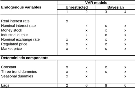
Additionally, I have vector autoregression models similar to those used in the Brazilian Central Bank (BCB) as auxiliary models for forecasting inflation. These models are presented in the Inflation Report of June 2004 and they are comprised by two unrestricted vector autoregressive models and two Bayesian vector autoregressive models for generating monthly forecasts for market price inflation.
The summary of the models’ specifications is displayed in the Table 5.18. A
common feature of all four models is the presence of three trend dummies included for capturing the period of disinflation process started with Plano Real in 1994.
The strategy for obtaining the forecasts of the Brazilian Central Bank models in my exercises differs from the data-rich models and autoregressive models described above. The h-month ahead forecasts from the VAR models are obtained by iterating monthly forecasts for h periods.
7
The market price index is obtained through the exclusion of the regulated and monitored prices from the IPCA.
8
I will use a strategy for the out-of-sample forecasting exercise similar to that used by Zaher (2005). First the models will be estimated initially on data from January 1995 to December 2000 and h-step ahead forecasts are computed. Then the estimation sample is augmented by 1-month, the model is reestimated and the corresponding h-step-ahead forecast is computed. I obtained inflation forecasts from January 2001 through July 2009. I also estimate the models using rolling regressions setting a fixed estimation window of 72 months.
This is not a strict real time analysis since I use current vintage data and assume the data are available in the time to run the forecast. Some variables, such as industrial production, are only available more than a month later and are subject to revisions.
In order to replicate the real-time problems associated with estimating seasonal factors, the variables are treated for seasonality for each period. Next, the data is standardized, and then the models are re-estimated and the factors are computed. Thus estimation procedure is entirely recursive in terms of parameters and factors, given the number of factors defined at a first stage.
6 - Empirical results
In this section we present the empirical results of our analysis. First we briefly describe the data we use and how the data are treated before used to obtain the factors using the principal components as well as the partial least squares.
Table 5.1 Specifications of VAR models used by Central Bank of Brazil
1 2 3 4
Real interest rate x
Nominal interest rate x x x
Money stock x x x
Industrial output x x x
Nominal exchange rate x x x x
Regulated price x x x x
Market price x x x x
Deterministic components
Constant x x x x
Three trend dummies x x x x
Seasonal dummies x x x
Lags 2 6 6 6
Source: Inflation Report, Central Bank of Brazil, June 2004
Endogenous variables
VAR models
6.1 - The Brazilian data
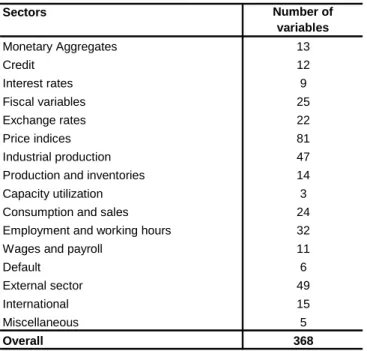
The collected data set for Brazil contains 368 monthly series over the sample period of January 1995 to July 2009. The sample was chosen to include only information after the Real Plan, a successful stabilization plan launched in June 1994. In order to obtain a balanced and as exhaustive as possible picture of the Brazilian economy, we included variety of economic variables related to prices (consumer, producer and retail prices and disaggregated by group of goods), labor market (employment, unemployment, wages and unit labor costs), output (industrial production and sales disaggregated by sectors) and income, monetary (aggregates: M2, M1, monetary base) and financial indicators (interest rates, stock prices), fiscal and external sector (effective and nominal exchange rates, imports exports and net trade), and other miscellaneous series. Table 6.1 provides a summary of the 368 variables employed in the factor estimation for the whole dataset.9
Following the standard procedures similar to those largely used in the empirical dynamic factor literature as in Marcellino, Stock and Watson (2003) and Artis, Banerjee and Marcellino (2005), the data are transformed in a multi-stage process.
1) Logarithms are taken of all nonnegative series and series characterized by
percentage changes, shares or rates such as unemployment and interest rates are transformed in the following way: ln(1+x/100);
2) The series are transformed to account for stochastic or deterministic trends
using Augmented Dickey-Fuller unit root test;
3) All series are tested for seasonality10 that consists of regressing each variable against eleven monthly indicator variables and if the F-Test on those eleven coefficients is significant at the 10% level of significance, the series is seasonally adjusted using X-12 program; and
4) Finally, in order to avoid scaling effects, the variables are transformed into
series with zero means and unit variance.
In order to verify whether the number of variables used to obtain the factor affects the estimation of the factors and the forecasting performance of the factor model,
9
The description of all series as well as the test results for stationary and seasonality is available upon request.
10
we used a method to keep only the series more related to the variable of interest. Our approach to reduce the initial dataset slightly differs from those discussed in Section 3.5. We performed Granger causality tests for all 368 series with respect to our variables of interest. Then we obtained the p-values for the F statistic of testing the null hypothesis whether the specific variable does not Granger-cause inflation. We discarded all variables for which the p-value is greater than 0.1. The number of variables for each forecast horizon is shown in Table 6.2.
In this paper all factor estimations are done for balanced dataset, therefore we do not include in our data either variables, which are not available for the entire sample or data with different frequency from monthly.11
11
In previous exercises we found that that balanced panel outperformed unbalanced panels in terms of the precision of the factor estimates.
Table 6.1 Summary of the variables employed in factors estimation
Sectors Number of variables Monetary Aggregates 13 Credit 12 Interest rates 9 Fiscal variables 25 Exchange rates 22 Price indices 81 Industrial production 47
Production and inventories 14
Capacity utilization 3
Consumption and sales 24
Employment and working hours 32
Wages and payroll 11
Default 6
External sector 49
International 15
Miscellaneous 5
As the variable of interest of Central Bank forecast models is the market price inflation, we perform our analysis using both the IPCA headline inflation and market price inflation. It allows us to compare the forecasting results from the factor models with the models used by the Brazilian Central Bank. As mentioned previously, in our forecasting setting the variable to be forecasted differs for each forecast horizon, therefore as I have five different forecasting horizons (1, 3, 6, 9 and 12 months), we have ten series to be forecasted.
6.2 Out-of-sample forecasting results
Aside from the Central Bank forecasts, all the forecasts we study are based on h-step-ahead linear projections as given by 5.1. I obtain the Central Bank’s VAR and BVAR forecasts by iterating monthly forecasts forwardly.
The forecasts are compared using a recursive simulated (pseudo) out-of-sample exercise. The forecast exercise is a two-step procedure; first we estimated the factors by principal components or partial least squares and then we use the estimate factors to obtain the forecasts.
I used the balanced model for some forecasting exercises. From equation (5.1), the factor or diffusion index forecasting function is given by:
(6.1) 8B 9B ∑"!:B8 ! ∑#!& ∑%!<#C#, ! for h = 1, 3, 6, 9 e 12
where C#, is the qth estimated factor with q =1, … r.
In order to check the optimal number of factor to be used in my analysis I extracted the factor using entire estimation sample (1995.1 to 2000.12) for the initial set of variables and for the targeted predictors for headline and market price inflation for the different forecast horizons. The numbers of estimated factor using the Bai and Ng information criteria given by equations 3.6 and 3.7 are given in Table 6.3. As one can notice, the number of factors varies from 3 to 10, and the second criterion (BNIC2) never assigns a higher number of factors than BNIC1 does. Take into account these results and also considering the question of parsimony, I decided to set a maximum number of factors equal to six and test the forecast accuracy for using different numbers of factors.
Thus, the PC, PTC and PLS models are estimated for the balanced panel with 1
≤ r ≤ 6 (number of factors) for, 0 ≤ m ≤ 4 (number of the lags for the factors) and 0 ≤ p
≤ 6 (number of the lags for inflation). The auto regressive model given by (6.3) is
similar to the factor model except for the exclusion of the factors terms.
(6.2) 8B 9B ∑"!:B8 !
Our forecasting exercises comprise two parts. In the first part, we compare the forecast performance of the factor models to autoregressive models for different forecasting horizons. Then we pick models with the best performances and compare their forecasts with the results from the vector autoregression models similar to those used in the Brazilian Central Bank.
6.2.1 Factor model forecasting performance
In this section we discuss the out-of-sample results comparing the forecasting provided by the three different methods (factor by principal component for the whole set of variables (PC) and for the targeted variables (TPC), and partial least squares (PLS)) against the benchmark (the best autoregressive model).
For each type of data-rich model (PC, PTC and PLS), our exercises are performed for the two relevant variables (headline and market price inflation) and using
two different e beforehand. Fo different specif component, and factors and fore
Figure 6
headline inflati approach. The for which half o horizon) presen RMSFE values than that of the
One ca verify, for exam usually outperf step ahead fore around 0.80 an results show t
t estimation appro For each one of cifications (changi and p= 1 to 4, the orecast horizon (1,
6.2 display the r
lation for each fo he results are show
lf of the models in sent a RMSFE equ
es lower than one he best autoregress
can observe some ample, that usuall erform the autoreg orecasts and the be and 0.85 in term that those mod
proaches (recursiv of these four cate nging m=1 to 6, th he number of lags (1, 3, 6, 9 and 12 st e relative RMSFE forecast horizon a own for the media in its category (sam equal to or less tha
ne means that the essive model.
e interesting resu ally the median pri regressive models e best results are fro
rms of relative RM odels hardly beat
sive and rolling re ategories we estim , the number of lag gs for the factors) g
steps ahead). FE of the out-of-n aout-of-nd out-of-number of dian models. The m same number of fa than that of this pa he specific model p
esults from the gr principal compone ls except in few ca from 6-step ahead RMSE. Concernin
eat the benchmar
regressions) as e timated the mode lags for the autore s) given specific nu
-sample forecasts of factor for the r e median model is factors for a given particular model. el presents a RMSF
graphs of Figure nent models (PC a cases for one-step ad forecasts mostly rning the PLS mo
ark models and
s explained del for 24 oregressive number of sts for the e recursive l is the one en forecast el. Relative SFE lower re 6.2. We and TPC) tep and 12-tly ranging odels, the d the best
performance is obtained for the 3-step ahead forecasts with the relative RMSE reaching slightly above 0.90.
Regarding the best number of factors to consider in forecasting, the answer should be four considering only PC models. For PTC models, the answer is not clear with advantage for model 1 or 6 factors. Finally, for PLS models, the best forecasting performance is obtained using 3 factors.
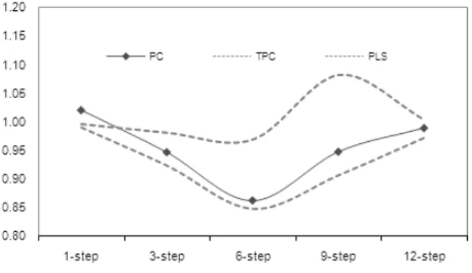
We notice that the median model of each method typically outperform the benchmark model. Additionally, for mostly models, the best results are found for 6-step ahead forecasts and the worst performance is verified for the one-step and 12-step forecasts. This behavior leads to a u-curve relating the average RMSE for median models and the forecasting horizons for the PC and TPC models s shown in Figure 6.3.
Figure 6.3 also shows that TPC provides better forecasts either in terms of
median models and the worst performance is provided by the PLS models.
The results for the rolling models are displayed in Figures 6.4 and 6.5. For this set of models, the best performance is still for the 6-step-ahead forecasts even for the PLS models.
From Figure 6.5 it is seen that TPC models show the best performance for shorter forecasting horizons (1 and 3-step ahead) whereas larger horizons are dominated by PC models.
Comparing the results in Figures 6.1 through 6.4, the rolling models seem to relatively outperform the recursive models in terms of RMSFE relative to the benchmark models. However, the comparison of the results is not straightforward since each group of models (recursive and rolling models) is compared to a benchmark model
estimated using the same approach as the group of models, that is, the benchmark for the rolling models is the best autoregressive model estimated by a rolling window.12
In my opinion, there are two remarkable features of the headline rolling models. First, PC and TPC models perform better for 12-step ahead forecasts than the same models in a recursive context. Additionally, the PLS model performance is largely improved in the rolling estimation making its forecasts competitive against those from PC and TPC models for 6-step ahead forecasts.
The general findings for the headline inflation cited above also apply for the market price inflation models as it can see in Figures A.1 through A.4 in the Appendix.
12
Actually, the RMSFE for the recursive benchmark models are usually lower than that for the rolling ones, and the recursive models tend to present a lower RMSFE when the benchmark is unified for the groups of models.
6.2.2 Comparing Central Bank’s and factor models for forecasting
In this section, I compare the factor models to vector autoregressive models that are similar to those the used in the Brazilian central bank. The comparison is performed for forecasts concerning the market price inflation since this is the variable of interest in the BCB auxiliary models.
Concerning the factor models, instead of using the median model, we chose the best model for each forecast horizon, that is, the one that that performs the best (minimum RMSFE) in the exercise we discussed in the previous subsection for each forecast horizon.
Therefore, in this subsection we analyze the results for the following models: the three set of factor models (PC, TPC and PLS), four models similar to those used by the Brazilian Central Bank (two VAR models: VAR1 and VAR2 and two Bayesian VAR models: BVAR1 and BVAR2) l. The analysis is carry out for five forecast horizons. It is important to notice that the factor models differ whereas the VAR and BVAR models are the same for all forecasts horizons.
The t-statistics of the Diebold-Mariano test for forecast accuracy for all 7 models are shown in Table 6.6. Positive (negative) values mean that the model in the row (column) presents a higher predictive accuracy than that of the model given by the column (row). Bold figures (italic figures) indicate that the statistic is significant at 5% (10%) significance level.
Among the unrestricted and TPC) usua for larger fore performance o principal comp regards the PC To form and Newbold ( predictive pow notice that the respect to the Furthermore, th
ng the VAR mode ted ones for most ually outperform t orecasting horizon of the PLS mod mponent models f
C model for 12-ste rmally test for for d (1998) test. Tabl
wer of the model the null hypothesis he VAR models i , the TPC model sh
dels, it is noticeab st forecast horizon
the other 5 mod ons. The best mo
odel is very poo s for almost all fo
step ahead forecas forecast encompas able 6.7 presents th el in the column w esis of no predicti s is almost alway l shows predictive p
eable the Bayesian ons. The principal odels and their rel model in this ex oor being statisti l forecasting horiz
asts).
passing, I will use s the p-values for t n with respect to th ictive power of th
ays rejected at 5 e power against all
ian VAR models d pal component mo relative advantage exercise is the T stically dominated rizons (the only e
se the Harvey, Le r the null hypothe the model in the the data-rich mod t 5% level o sign all other models.
ls dominate models (PC ge is larger TPC. The ted by the exception Leybourne, thesis of no he row. We odels with ignificance.
7. Concluding remarks
In this paper I sought to verify if using methods that use a large number of variables we can improve the forecasts of inflation. I used three different approaches: factor model with principal component with and without targeted variables and partial least squares.
All the results presented above indicated that in a rich data environment, the use of models that use the information of a large number of variables for forecasting inflation is very promising. Nevertheless, using a large dataset available does not imply that the forecasting performance will be better, since I found that reducing the number of series based on granger causality tests can lead to improvements in the forecast ability of the models.
Concerning different forecasting horizons, the best results in terms of relative forecasting performance for the principal component forecast models are usually for 6-step ahead forecasts.
I find that the factor model outperforms the alternative models and can function as a useful complement to the Brazilian central bank’s current forecasting tools, especially at longer horizons. Furthermore, the proposed data-reduction rule provides superior forecasts at some horizons.
As a preliminary study, this work could be extended in several ways. As the use of large data set seems to be worthwhile, I intend to combine data with different frequencies as well as to include series with missing values. This can approximate my forecasting exercises to what forecasters do in real-time. Furthermore, it would be interesting to include other methods to estimate factor models and to use other rich-data approaches such as Bayesian model averaging (BMA). I want to use different algorithms to obtain the PLS factors such as those provided by the statistical package SAS. Additionally, as “targeting” the variables seemed to work well in terms of forecasting improvement, it will be also interesting to verify how other methods of pre-selecting the variables would work. Finally, in order to verify how robust the results obtained so far are, I intend to test the performance of the model using different samples for the forecasting horizon.
References
Aguirre, A., L. F. Céspedes (2004), “Uso de análisis factorial dinámico para proyecciones macroeconómicas”, Workings Papers Central Bank of Chile 274. Altissimo, F., A. Bassanetti, R. Cristadoro, M. Forni, M. Hallin, M. Lippi, L. Reichlin
(2001), “EuroCOIN: a real time coincident indicator of the euro area business cycle”, CEPR Working Paper 3108.
Angelini, E. and Henry, J. and Mestre, R. (2001), “Diffusion index-based inflation forecasts for the euro area”, Working Paper 61, European Central Bank.
Artis, M., Banerjee, A. and Marcelino, M. (2005) “Factor forecast for the UK”. Journal
of Forecasting, 24(4), 279-298.
Atkeson, A., and Ohanian, L. (2001). "Are Phillips Curves Useful for Forecasting Inflation?" FRB Minneapolis Quarterly Review (Winter) pp. 2-11.
Bai, J. and Ng, S. (2002), “Determining the Number of Factors in Approximate Factor Models”, Econometrica 70(1), 191-221.
Bai, J. and Ng, S. (2008), "Forecasting economic time series using targeted predictors,"
Journal of Econometrics, Elsevier, vol. 146(2), pages 304-317, October.
Banerjee, A., M. Marcellino, I. Masten (2005), “Leading indicators for euro-area inflation and GDP growth.”, Oxford Bulletin of Economics and Statistics, 67, 785-814.
Banerjee, A., M. Marcellino, I. Masten (2006), “Forecasting macroeconomic variables for the new member states” in: Artis, M.J., A. Banerjee, M. Marcellino (eds.), The central and eastern European countries and the European Union, Cambridge University Press, Cambridge, Chapter 4, 108-134.
Bates, J. M. and Granger, C.W.J. (1969). “The Combination of Forecasts.” Operations
Research Quarterly, 20, 451-469.
Bernanke, B. and Boivin, J. (2003). "Monetary policy in a data-rich environment,"
Journal of Monetary Economics, Elsevier, vol. 50(3), pages 525-546.
Boivin, J., and Ng, S. (2005). “Understanding and comparing factor-based forecasts”,
International Journal of Central Banking, 1, 117-151.
Boivin, J., S. Ng (2006), “Are more data always better for factor analysis”, Journal of
Econometrics, 132, 169-194.
Boivin, J., and M. Giannoni (2006), “DSGE Models in a Data-Rich Environment,” NBER Working Papers 12772, National Bureau of Economic Research, Inc.
Breitung, J., S. Eickmeier (2006), “Dynamic factor models”, in: O. Hübler and J. Frohn (Eds.), Modern econometric analysis, Chapter 3, Springer 2006.
Bruneau, C., O. de Bandt, A. Flageollet (2003a), “Forecasting inflation in the euro area”, Banque de France NER 102.
Camacho, M. and Sancho, I. (2003). “Spanish Diffusion indexes”. Spanish Economic
Review, 5.
Cecchetti, S, Chu, R. and Steindel, S. (2000). "The unreliability of inflation indicators," Current Issues in Economics and Finance, Federal Reserve Bank of New York, issue Apr.