Variable Selection and Inference for Multi-period Forecasting Problems

Variable Selection and Inference for Multi-period

Forecasting Problems

M.

H

ASHEM

P

ESARAN

A

NDREAS

P

ICK

A

LLAN

T

IMMERMANN

CES

IFO

W

ORKING

P

APER

N

O

.

2543

CATEGORY 10: EMPIRICAL AND THEORETICAL METHODS

FEBRUARY 2009

An electronic version of the paper may be downloaded

• from the SSRN website: www.SSRN.com

• from the RePEc website: www.RePEc.org

CESifo

Working Paper No. 2543

Variable Selection and Inference for Multi-period

Forecasting Problems

Abstract

This paper conducts a broad-based comparison of iterated and direct multi-step forecasting

approaches applied to both univariate and multivariate models. Theoretical results and Monte

Carlo simulations suggest that iterated forecasts dominate direct forecasts when estimation

error is a first-order concern, i.e. in small samples and for long forecast horizons. Conversely,

direct forecasts may dominate in the presence of dynamic model misspecification. Empirical

analysis of the set of 170 variables studied by Marcellino, Stock and Watson (2006) shows

that multivariate information, introduced through a parsimonious factor-augmented vector

autoregression approach, improves forecasting performance for many variables, particularly at

short horizons.

M. Hashem Pesaran

Faculty of Economics

Cambridge University

Sidgwick Avenue

Cambridge, CB3 9DD

United Kingdom

[email protected]

Andreas Pick

De Nederlandsche Bank and

Faculty of Economics

Cambridge University

Sidgwick Avenue

Uk - Cambridge, CB3 9DD

[email protected]

Allan Timmermann

University of California San Diego

Rady School of Management

Otterson Hall, Room 4S146

9500 Gilman Dr. #0553

USA - La Jolla, CA 92093-0553

[email protected]

January 26, 2009

We thank Alessio Sancetta and seminar participants at the 2008 Rio Forecasting Conference

at Fundacao Getulio Vargas for comments and suggestions on the paper. Timmermann

acknowledges support from CREATES, funded by the Danish National Research Foundation.

This paper was written while the second author was Sinopia Research Fellow at the

University of Cambridge. He acknowledges financial support from Sinopia, quantitative

specialist of HSBC Global Asset Management. The opinions expressed in this paper do not

1

Introduction

Economists are commonly asked to forecast uncertain outcomes multiple periods ahead in time. For example, in a recession state a policy maker may want to know when the economy will recover and so is interested in forecasts of output growth for, say, horizons of 1, 3, 6, 12, and 24 months. Similarly, fixed-income investors are interested in comparing forecasts of spot rates multiple periods ahead against current long-term interest rates in order to arrive at an optimal investment strategy.

Given the importance of the horizon to many forecasting problems, it is not surprising that a substantial literature has considered the multi-step forecasting problem, see Cox (1961), Brown and Mariano (1989), Clements and Hendry (1998), Findley (1983), Schorfheide (2005), and Ullah (2004), with Bhansali (1999) providing a survey, and Ing (2003) giving asymptotic results for stationary ARs.

Two basic strategies exist for generating multi-period forecasts. The first approach is to estimate a dynamic model for data observed at the highest available frequency, e.g. monthly, and then use the chain rule to generate a forecast at the desired horizon,h≥1. Under this “iterated” or “indirect” ap-proach, the forecasting specification is the same across all forecast horizons; only the number of iterations changes withh. In the context of univariate specifications, typically autoregressive models are used to this end, while if multivariate specifications are considered, vector autoregressions must be used. The second approach is to estimate a model for the variable mea-sured h-periods ahead as a function of current information. This leads to so-called “direct” forecasts. Under this approach, the forecasting model and its estimates will typically vary across different forecast horizons.

Each approach has advantages and drawbacks. For a given model the iterated approach leads to more efficient estimates since it makes use of data recorded at the highest available frequency and so uses the largest available sample size. Conversely, if the model is misspecified, due, for example, to using an incorrect lag order, iterating the model multiple steps ahead can attenuate any existing biases. Direct forecasts are less efficient, but also more likely to be robust to model misspecification as they are typically linear projections of current realizations on past data. Direct forecasts introduce new problems, however, due to the overlap in data resulting from h > 1, which affect the covariance of the forecast errors.

Given such trade-offs, which approach delivers the best forecasts, the direct or the iterated, is therefore ultimately an empirical question. For univariate forecasting problems, as pointed out by Marcellino, Stock and Watson (2006) the performance of the two methods will depend on the sample size, forecast horizon and method used to select lag lengths for the forecasting models. In a multivariate setting it also becomes important how the potentially high-dimensional variable selection search is conducted and how multi-step forecasts of additional predictor variables are generated.

For multivariate specifications of even modest dimension, a global model specification search very rapidly becomes intractable unless the problem is further constrained: withdpotential regressors, there are 2ddifferent linear models and with d easily in the hundreds it is infeasible to evaluate every possible model.

To deal with this dimensionality problem, we propose a factor-augmented VAR approach to iterated forecasting that builds on the work by Bernanke, Boivin and Eliasz (2005) and Stock and Watson (2005). This limits the model specification search to consider inclusion of only a few common fac-tors extracted from different categories of economic variables such as in-come/output, employment, construction/inventories, interest rates/asset prices and nominal prices/wages. This means that in addition to past values of the predicted variable itself relatively few potential predictors need to be considered.

How close the best forecasting models approximate the “true” data gen-erating process also plays a role since model misspecification can change the relative performance of the iterated and direct forecasts. Finally, we show that how the direct forecasts account for data overlap can affect the results. We propose modifications to existing model selection methods that account for such data overlap.

Empirically, we confirm the finding reported by Marcellino, Stock and Watson (2006) that the iterated forecasts are best overall among the uni-variate forecasting methods. However, we also find that forecasts generated by the factor-augmented VARs generally perform better than the univari-ate forecasts, the important exception being variables tracking prices and wages. This suggests that it is helpful to extend the forecasting models beyond purely univariate schemes and include multivariate information.

The main contributions of the paper are as follows: First, for simple dynamic models such as the AR(1) specification we present a new theoretical result establishing conditions under which both the iterated and the direct forecasts are unconditionally unbiased. A key condition turns out to be symmetry of the innovations. Second, we extend existing model selection criteria such as the AIC and the BIC to account for the overlap introduced by the direct forecasting method which affects the covariance of the forecast errors and so can lead to different models being chosen in small samples. Third, we undertake a comprehensive study of model selection methods and shed light, both through Monte Carlo simulations and through empirical results, on which approach works best in the recursive modeling of a variety of economic variables. We consider univariate models as well as multivariate factor augmented vector autoregressive specifications hitherto not used in the context of direct and indirect multi-period forecast comparisons.

The outline of the paper is as follows. Section 2 discusses the theoretical trade-offs associated with direct versus iterated forecasts. Section 3 sets up the forecasting problem for the univariate and multivariate case, while

Sec-tion 4 deals with the model selecSec-tion issue. SecSec-tion 5 presents some Monte Carlo results, while Section 6 describes our empirical findings using the data originally analyzed by Marcellino, Stock and Watson (2006). Section 7 con-cludes. Technical results are provided in appendices.

2

Comparison of Direct and Iterated Forecasts for

the AR(1) Model

In this section we introduce the iterated and direct forecasting approaches in the context of the simplest possible dynamic model, namely an AR(1) speci-fication. Next, we establish a new result showing that both approaches lead to forecasts that are unconditionally unbiased provided that the innovations to the underlying data generating process are symmetrically distributed. Fi-nally, we characterize the relative efficiency of the two approaches in finite samples.

The analysis is conducted under the assumption that a stationary AR(1) model of the following form is the correct specification:

yt=a+φyt−1+εt, |φ|<1, εt∼iid(0, σε2). (1) Lettingµ=a/(1−φ), we can use the equivalent representation

yt = µ+ut, where (2) ut = ∞ X i=0 biεt−i, bi=φi.

Alternatively, for purposes of the direct forecasting approach that projects yt onyt−h, we can write yt = a µ 1−φh 1−φ ¶ +φhyt−h+vt, (3) ≡ ah+φhyt−h+vt, where vt = h−1 X j=0 φjεt−j.

Notice that v_t will follow an M A(h−1) process even when ε_t is serially uncorrelated due to the data overlap resulting fromh >1.

2.1 Iterated and Direct Approach

Suppose that we are interested in forecastingy_T+h based on information up to periodT and that theT+hobservationsyt, t=−h+ 1,−h+ 2, . . . , T are available for model estimation. Denote theh-step ahead forecast ofyT+hby

ˆ

yT+h if the iterated procedure is used, and by ˜yT+h if the direct method is employed.

Under the iterated procedure ˆ y_T+h = ˆa_T Ã 1−φˆh T 1−φˆ_T ! + ˆφh_Ty_T, (4)

where ˆa_T and ˆφ_T are the estimators of a and φ obtained from the OLS regression (1) of yt on an intercept and yt−1 using the observations yt, t =

−h+ 1,−h+ 2, . . . , T.

The direct forecast ofy_T+h is given by

˜

y_T+h= ˜a_h,T + ˜φ_h,TyT, (5)

where ˜ah,T and ˜φh,T are the OLS estimators of ah and φh obtained from the regression (3) of yt on an intercept and yt−h using the same sample observations,yt, t=−h+ 1,−h+ 2, . . . , T.

Specifically, under the iterated method, (T+h−1)−1 T X t=−h+2 yt= ˆaT + ˆφT(T+h−1)−1 T X t=−h+2 yt−1, or, equivalently, ¯ yh:T = ˆaT + ˆφT y¯h:T,−1, (6) where ˆ φT = P_T t=−h+2yt(yt−1−y¯h:T,−1) P_T t=−h+2(yt−1−y¯h:T,−1)2 . Similarly, for the direct method we have

T−1 T X t=1 y_t= ˜a_h,T + ˜φ_h,TT−1 T X t=1 y_t−h,

or, equivalently (noting that ¯yT = ¯y1:T),

¯ yT = ˜ah,T + ˜φh,Ty¯T,−h, (7) where ˜ φh,T = P_T t=1yt(yt−h−y¯T,−h) P_T t=1(yt−h−y¯T,−h)2 . (8)

We next establish conditions under which both the direct and indirect forecasts are unconditionally unbiased:

Proposition 1 Suppose data is generated by the stationary AR(1) process, (1) and define the h-step ahead forecast errors from the iterated and direct methods, ˆ eT+h=yT+h−yˆT+h, and ˜ e_T+h=y_T+h−y˜_T+h,

where the iterated h-step forecast, yˆ_T+h, and the direct forecast, y˜_T+h, are given, for example, by (4) and (5), respectively. Assume that ut and vt,

defined in (2) and (3), are symmetrically distributed around zero, have finite second-order moments and expectations ofφˆ_T and φ˜_h,T exist. Then for any finite T andh we have

E(ˆe_T+h) = E(˜e_T+h) = 0.

A proof of this proposition is provided in Appendix A.

The result is surprising since neither set of estimators (ˆaT, ˆφT) and (˜a_h,T,φ˜_h,T) is unbiased. However, the main intuition behind the results follows from the fact that, under the stated assumptions,

E(ˆµ_T −µ) = 0, and E µ ˆ a_T 1−φˆ_T ¶ = a 1−φ.

The proposition generalizes the known result in the literature for h= 1 established, for example, by Fuller (1996) to multi-step ahead forecasts. For h= 1,Pesaran and Timmermann (2005) also show that forecast errors are unconditionally unbiased for symmetrically distributed error processes even in the presence of breaks in the autocorrelation coefficient, φ, so long as µ is stable over the estimation sample.

Notice that the result holds only unconditionally and that the direct and iterated forecasts are not typically conditionally unbiased for a given value ofyT 6=µ, as noted by Phillips (1987).

In comparing the iterated and direct forecasts it is worth noting that when φ is positive and not too close to unity, for even moderately large values of h, ˆφh_T ≈ 0, since ˆφT < φ. It follows that in such cases, ˆeT+h = (µ−µˆT) +vT+h+o(φh). Similarly, ˜eT+h =−v¯T +vT+h+o(φh).Hence, for h moderately large andφ not too close to the unit circle, a measure of the relative efficiency of the two forecasting approaches can be obtained:

E(ˆe2 T+h) E(˜e2 T+h) = E(ˆµT −µ) 2_{+ E(v}2 T+h) +o(φh) E(¯v2 T) + E(vT2+h) +o(φh) , (9)

since (µ−µˆT) and ¯vT are uncorrelated withvT+h. But E(µ−µˆT)2 =O(T−1) and does not depend onh. To derive E(¯v2

T),recall that vt = P_h−1

j=0φjεt−j, and hence after some algebra

T v¯T = h−1 X j=1 µ 1−φj 1−φ ¶ φh−jε_−h+j+1+ µ 1−φh 1−φ ¶T−_Xh+1 t=1 εt+ h−1 X j=1 µ 1−φj 1−φ ¶ εT−j+1, and E(¯v_T2) = Var(¯vT) = σ2 ε T2    h−1 X j=1 µ 1−φj 1−φ ¶_2h 1 +φ2(h−j) i + µ 1−φh 1−φ ¶₂ (T−h+ 1)   . Clearly, E(¯v2

T) =O(T−1) ifh is fixed. But it is easily seen that we continue to have E(¯v2

T) = O(T−1) even ifh → ∞ so long as h/T →κ, where κ is a fixed finite fraction in the range [0,1). Therefore,

E(ˆe2 T+h) E(˜e2

T+h)

= 1 +O(T−1) +o(φh),

and forT sufficiently large there will be little to choose between the iterated and the direct procedures.

This analysis suggests two points. First, we should expect to find the greatest difference between the performance of the two forecasting methods in small samples (T) or in situations wherehis large, i.e. whenh/T is large. Second, in the context of correctly specified dynamic models there is little reason to choose one approach over the other in large samples or whenh/T is small.

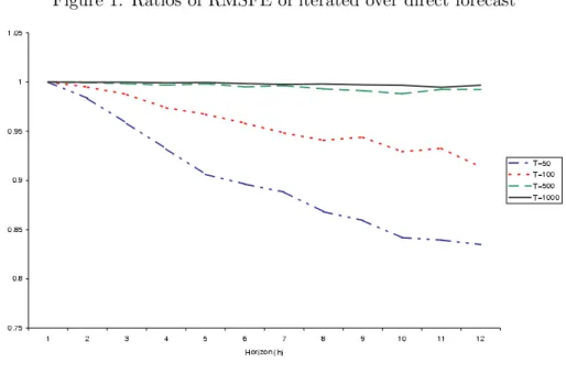
To illustrate these results, Figure 1 plots the ratio of RMSE values of the iterated over the direct forecasting approaches forh= 1,2, . . . ,12,assuming φ= 0.9 and using sample sizes of T = 50, 100, 500, and 1000. The relative efficiency of the iterated approach is very pronounced whenT is small orhis large. This is to be expected since the estimation error associated with the direct approach is larger in this situation. Notice also that the advantage of the iterated approach rapidly gets reduced as the sample size is expanded or the forecast horizon is shortened.

In line with the existing literature, the above results conditioned on a given model, namely the AR(1) specification in (1), while ignoring the effect of model misspecification and model uncertainty. It is not clear how to obtain finite-sample analytical results without conditioning on a particular model specification. To deal with this important issue, we next discuss the types of forecasting models under consideration and then turn to a variety of methods for model selection.

Figure 1: Ratios of RMSFE of iterated over direct forecast

3

Methods for Multi-period Forecasting

Suppose a forecaster is interested in predicting a k×1 vector of target variables y_t= (y1t, y2t, . . . , ykt)0 by means of their own past values and the past values of an additional set of potentially relevant predictor variables, xt= (x1t, x2t, . . . , xM t)0. Typicallyk is small, often 1 or 2, butM could be large.

For purposes of calculating one-step-ahead forecasts under the iterated approach, the regressors are treated as conditional information and so how they are generated is not a concern. This also holds under the direct fore-casting approach irrespective of the forecast horizon. In contrast, when applying the iterated forecasting approach to multi-period horizons,h >1, the regressors themselves need to be predicted since such values in turn are required to predict future values ofy.

3.1 Factor-Augmented VARs

In cases where M is relatively small, say less than ten, one approach is to treat all variables simultaneously, i.e. model z_t = (y0

t,x0t)0. Multi-period forecasts ofytcan then be obtained iteratively using a conventional VAR of the form zt=µz+ µ Ap(L) Bq(L) Cr(L) Ds(L) ¶ zt−1+ξt, (10) where p and q are the lag order of y_t and xt in the equation for yt and r and sis the lag order ofy_t and xt in the equation forxt.

However, in the common situation where the time-series dimension of the data is limited while M is large, this approach is unlikely to be successful due to the high dimension of the coefficient matrices of the VARs, i.e.Cr(L) and Bq(L) in particular.

To deal with this issue, a conditional factor-augmentation approach can be used. In this approach, the large-dimensionalxt-vector is condensed into a subset of factors, ˆf_t, of dimensionm < M, used to summarize the salient features of the larger-dimensional data. A factor-augmented VAR based on the variablesz˜t= (y0t,fˆ

0

t)0 can then be used: ˜ zt=µz+ µ A_p(L) C_q(L) 0 D∗_s(L) ¶ ˜ zt−1+ξt. (11)

Notice the asymmetric treatment ofy_tand ˆf_t under this approach. Due to the zero in the lower left corner of the lag polynomial matrix pre-multiplying ˜

zt−1, future values of the factors are generated using only current and past values of the factors themselves. The y-variables are therefore not used to predict the factors, while the factors are used to predict they-variables.

Only those factors that help predict y_t are relevant and should be in-cluded in this model. This may be a subset of the full set of factors under consideration, which we denote by ˆf∗_t. One then has to choose whether to use the full set of factors ˆf_t to predict the subset of factors, ˆf∗_t, selected when forecastingy_t+h,or whether to use only lagged values of ˆf∗_t to predict their future values. The choice would depend on the number of available factors. In the empirical application below where we consider five factors we shall be using all the factors in forecasting future values of ˆf∗_t.

3.2 Multi-step Forecasts with Dynamic Factor Models

Assume that thek×1 vector of target variables,y_t, is generated according to the following dynamic factor model

y_t=µ+Ay_t−1+Γ1ft−1+εt, (12)

εt∼iid(0,Σ),

wheref_tis a vector of unobserved common factors, whileA,Γ1, andΣare unknown coefficient matrices.

In order to forecast y_T+h given information at time T we also need to forecast the factors. Despite the dynamic nature of the above model, we follow Stock and Watson (2002) and estimate f_t by the principal compo-nent (PC) procedure, although one could equally employ the dynamic factor approach of Forni et al. (2005). The key question when using factor models is the choice of the number of factors. This can be determined, for example, using the information criteria (IC) proposed by Bai and Ng (2002). In prac-tice there is a considerable degree of uncertainty surrounding the number of

factors to be used, and as pointed out by Bai and Ng (2009), the IC assume that the factors are ordered as predictors of the regressors x_t, an ordering that might not be appropriate for predicting the target variables, yt. The resultant factors are also often difficult to associate with readily understood economic concepts.

In view of these concerns we adopt a hierarchical approach where we first divide the 170 variables into five economically distinct groups and then select the first PC from each of the categories. All the computations are carried out recursively, so that no future information is used in the construction of the factors. We denote the recursively estimated PC’s by ˆf_t(T−w+ 1 :T), whereT ≥t is the time at which factors are computed and wis the size of the estimation window used to do the computations. To simplify notations we denote ˆf_t(T−w+1 :T) by ˆf_t, although strictly speaking both subscripts are needed for appropriate timing when carrying out the computations.1

3.3 Iterated System Forecasts

For multivariate forecasts we first select the relevant subset of factors and the lag lengthspand q using the conditional model:

y_t=µ_y+Ap(L)yt−1+Cq(L)ˆft−1+ut, (13) where

Ap(L) = A0+A1L . . .+Ap−1Lp−1,

Cq(L) = C0+C1L+. . .+Cq−1Lq−1.

We determine the lag ordersp and q and the subset of m∗ _{factors from the} total set of m factors by applying information criteria to the likelihood of

y_t.

For simplicity, we obtain forecasts only from the full set of m factors. Hence we first select a VAR(s) model in ˆf_t so the value of swill be deter-mined by AIC or BIC, again applied recursively. Then

ˆ

f_t=µ_f +Ds(L)ˆft−1+νt, (14) where

Ds(L) =D0+D1L+. . .+Ds−1Ls−1.

To computeh−step-ahead forecasts ofy_t, the conditional and marginal models need to be combined:

y_t = µ_y+A_p(L)y_t−1+C∗_q(L)ˆf_t−1+u_t, ˆ

f_t = µ_f +D_s(L)ˆf_t−1+ν_t,

1_{In the case of an expanding estimation window (withw =T) one would setT =t}

or, definingzt= (y0t,fˆ 0 t)0 and ξt= (u0t,ν0t)0, we have z_t= µ µ_y µ_f ¶ + µ Ap(L) C∗q(L) 0 Ds(L) ¶ z_t−1+ξ_t. (15)

where the selection of factors in the conditional model (13) is reflected in zero-restrictions inC∗₁,C∗₂, . . .C∗_q, where the columns corresponding to the factors that are not selected are set to zeros. The factor-augmented VAR in

zt, (15), can then be iterated forward.2

3.4 Univariate Forecasts

Univariate forecasts are a special case of the multivariate forecasts described above. Nevertheless, it is worth briefly clarifying how the forecasts are computed for these models.

For example, withp lags the iterated forecast ofyT+h given information at timeT is

ˆ

yT+h= ˆα+ ˆβ1yˆT+h−1+ ˆβ2yT+h−2+. . .+ ˆβpyT+h−p,

where ˆy_T+h−1=y_T+h−j ifh≤jand the parameters are estimated from the regression model

yt=α+β1yt−1+β2yt−2+. . .+βpyt−p+εt, t=T−w+ 1 +p, T −w+ 2 +p, . . . , T.

Under the direct approach, for a given lag length,p, the parameters are estimated from the regression

y_t=α+β₁y_t−h+β₂y_t−h−1+. . .+β_py_t−h−p+ε_t, and the forecast is

ˆ

y_T+h= ˆα+ ˆβ1yT + ˆβ2yT−1+. . .+ ˆβpyT−p.

4

Model Selection

Given the large dimension of the set of potentially relevant predictor vari-ables, how a particular model is chosen by the forecaster is of great im-portance. We consider two basic model selection criteria, namely AIC and BIC. Both criteria are commonly used in forecasting studies and have well known properties: AIC achieves a good approximate model as the sample

2_{Alternatively, one could model only the factors that have been selected in the}

condi-tional model (13). This may be less efficient than using the full VAR in (14), but a smaller number of parameters needs to be estimated from a finite number of observations. It is therefore not cleara priori which approach will perform better.

size expands even if the true model is not contained in the universe of models under consideration. However, AIC is not a consistent criterion in the sense that, asymptotically, it does not select the true model with probability one if it happens to be included in the search. In contrast, BIC is a consistent model selection criterion.

The iterated forecasting models can be selected either on the basis of single equations or using a system of equations. For the direct forecasting models a decision has to be made whether or not to correct for the overlap in the observations that affects the sample covariance matrix of the forecast errors, although such corrections will be of second order importance in large samples.

4.1 Iterated Forecasts

Models used to generate the iterated forecasts are selected based on the following criteria. First, we consider applying AIC or BIC to the single equation (k= 1) containing the variable of interest, i.e. for AIC:

AIC = ln[ˆu0_iuˆi/(T−1)] +_T2₋d₁, (16) where ˆui is a (T −1)×1 vector of estimated residuals with typical element

ˆ

uit =y1,t−βˆiT0 xt−1, t= 2,3, . . . , T,

while the d×1 vector xt−1 contains subset i of y1t−1 and ft−1 and their lags andβˆ_T is estimated using observations up toT. Similarly, for BIC,

BIC = ln[ˆu0_iuˆi/(T−1)] + ln(_TT₋−₁1)d, (17) where ˆu_i is defined as above.

For k >1, we have

AIC = ln|Σˆ_i|+ 2kd

T−1 (18)

where ˆΣis the k×kestimated error covariance matrix ˆ

Σi = _T 1₋₁(Y0Y −Y0Xi(X0iXi)−1X0iY),

Y is the T −1×k matrix of stacked y_t = (y1t, y2t, . . . , ykt)0, and Xi is the observation matrix formed from stacking x_it−1 over the observations, t= 2,3, . . . , T. Similarly,

BIC = ln|Σˆ_i|+ln(T −1)kd

4.2 Direct Forecasts

The direct forecasting models are selected based on either AIC AIC = ln[ˆu0_huˆ_h/(T−h)] + 2d

T−h (20)

where ˆu_h is a (T−h)×1 vector of estimated residuals with typical element ˆ

uit=y1t−βˆiT0 xt−1, t=h+ 1, . . . , T, or, using BIC,

BIC = ln[ˆu0_huˆh/(T−h)] + ln(_TT₋−_hh)d, (21) where ˆuh is defined as above.

For h > 1 the overlap of the forecasts will produce considerable auto-correlation in the residuals. This should be accounted for in small samples when calculating the information criteria. Here we consider two ways to calculate the corrections with further details given in Appendix B. The first approach is to make use of the modified information criteria defined by

AICΠ = ln[ˆu0huˆh/(T−h)] + 2tr ³ ˆ Π_S ´ T −h (22) BICΠ = ln[ˆu0huˆh/(T−h)] + ln(T−h)tr ³ ˆ ΠS ´ T−h , using ˆ ΠS = (X0X)−1X0SX/h

whereS is a matrix withhon the diagonal,h−1 on the first diagonal above and below the main diagonal,h−2 on the second diagonal above and below the main diagonal, and so on, i.e.

S =           h h−1 h−2 . . . 0 h−1 h h−1 . . . 0 h−2 h−1 h ... .. . . .. h−1 h−2 0 . . . h−1 h h−1 0 . . . h−2 h−1 h           .

This formulation aims at capturing theM A(h−1) form of the error process of the overlapping regressions but assumes that the serial correlation of the underlying (non-overlapping) observations is negligible.

The second approach uses an estimated covariance matrix. In particular, we use the Newey-West (1987) covariance matrix to obtain the correction. This yields the modified AIC and BIC:

AIC_Π˜ = ln[ˆu0huˆh/(T −h)] + 2tr ³ ˜ Π ´ T −h (23) BIC_Π˜ = ln[ˆu0huˆh/(T −h)] + ln(T −h)tr ³ ˜ Π ´ T−h , where Π˜ = ˆΣ−_xx1Ωˆ, ˆΣ_xx = ˆσ2³X0_X T−h ´

, ˆΩ is the long-run variance of the residuals as estimated by the Newey-West covariance matrix with bandwidth set to min(h, T1/3_).

5

Monte Carlo Simulations

Having described the forecasting setup and the model selection methods, we next turn to Monte Carlo simulation as a means to evaluate the performance of the various model selection and estimation approaches under two data generating processes (DGPs). Both data generating processes assume the following VAR model fory_t= (y1t, y2t, . . . , ykt)0:

y_t=µ+αAy_t−1+H_εε_t, ε_t∼N(0,I_k). (24) The goodness of fit is controlled by the scaling parameter α, which is set such that the population R2 _{= 0.2 or R}2 _{= 0.8, representing low and high} predictability scenarios, respectively. An alternative would be to vary Hε. However, for the purpose of controlling the goodness of fit of the equations and given the choices to be considered forA, it has proved more convenient to vary α and set Hε=Ik. Data are generated for samples of T = 60 ,120, and 240 observations which in turn are used to generate forecasts for periodT+h, soT corresponds tow, the length of a rolling window used for estimation. We consider forecast horizons ofh= 1, 3, 6, 12, and 24 periods. The first DGP assumes that all variables contain useful information for predicting the variable of interest (always the first variable) and so the one-step-ahead forecast should select all variables. Under the second DGP, it-erated multi-step forecasts can be expected to be inefficient because they select models that produce good one-step-ahead forecasts and a variable in the DGP is only helpful for longer horizon forecasts.

Data Generating Process 1

Under the first DGP, we setk= 3 withµ=0, and choose theA-matrix as follows A=   0₀.8 ₀0_..₉₅5 0₀.5 0 0 0.7  _,

so that both y2 and y3 help predict y1, but y2t and y3 are in turn not themselves predictable by means of past values ofy₁. Moreover,y₂ is highly persistent whiley3 is not, suggesting that for large values ofhin particular, y2 should play more of a role in forecastingy1 as compared to y3.

Data Generating Process 2

The parameters for the second DGP are set tok= 4,µ=0, and

A=     0.8 0.5 0 0 0 0.8 0.5 0 0 0 0.9 0.5 0 0 0 0.95    ,

Notice that y2 helps predict y1, but y2 is in turn not itself predictable by means of past values of y1. Moreover, y3 neither predicts nor is predicted by y1 but y3 predicts y2 and therefore may help predict y1 over medium horizons. Finally, the most persistent variable, y4, indirectly helps predict y1 through its ability to predicty3.

5.1 Forecasts

We generate forecasts from both univariate and multivariate models. The univariate forecasts are based on AR models with lag length up topmax = 12. The multivariate models consider all regressors in the DGPs with the maximum lag length restricted topmax= 2.

In each case forecasts are based on the model selected by one of the cri-teria discussed in the previous section. Iterated forecasts are then calculated as follows:

ˆ

Z∗_T+h = ˆµ(I+ ˆA+· · ·+ ˆAh−1) + ˆAhz∗_T, (25) wherez∗

t is the sub-vector ofztchosen in the model selection step,Z∗t =z∗t ifz∗

t includes y1t orZ∗t = (y1t,z∗t) ifz∗t does not include y1t, and ˆµ=0 if the intercept is not selected.

Direct forecasts are obtained from ˜

y_1,T+h = ˆβ0_hxs,T, (26)

wherexs,T is the subset of regressors that are selected, i.e.,xs,T =z∗T if the intercept is not selected orxs,T = (1,z∗_T) if the intercept is selected.

The forecast errors are calculated as ˆ

e_T+h = y_1,T+h−yˆ_1,T+h or ˜

e_T+h = y_1,T+h−y˜_1,T+h (27)

depending on whether the iterated or direct forecasts are used. Finally, the forecasting performance is measured by the mean squared forecast error (MSFE) computed as MSFE = 1 R R X r=1 e2_T+h,r, (28)

where r = 1,2, . . . , R denotes the Monte Carlo replications and e_T+h is either ˆeT+h or ˜eT+h.

5.2 Summary of Results

Results from the Monte Carlo simulations are reported in Tables 1 and 2. In order to study how the degree of predictability affects the findings, each table contains a panel withR2 _{= 0.2 and a panel withR}2_{= 0.8.The former} is closer to the empirical results that we obtain, while the second scenario is more relevant for some of the highly persistent variables.

First consider the results for the data generated under DGP 1. For both the univariate models and the VARs, the iterated approach dominates the direct approach. This is a robust finding that holds across sample sizes (T = 60, 120, and 240), information criteria (AIC versus BIC), and forecast horizons (h = 3,6,12, and 24). As expected the relative performance of the direct to the iterated forecasts improves with the sample size, T, since it becomes less costly to use an inefficient estimation method in the larger samples.

Turning to a comparison of the univariate and multivariate forecasts, the picture is less clear-cut. In many cases the best overall forecast is generated by the VAR models, although this depends on the degree of predictability assumed for the DGP. Assuming weak predictability (R2 _{= 0.2), under the} iterated approach VAR-models selected by the simple AIC or BIC gener-ally produce better forecasts than their univariate counterparts. This holds across all forecast horizons when T = 60 or T = 120. The performance of the VAR forecasts gets even better relative to the univariate forecasts when the level of predictability is raised by setting R2 = 0.8. In this case the VAR-forecasts generate lower MSFE-values than the corresponding uni-variate forecasts for the vast majority of horizons and sample sizes. These results suggest that the multivariate VAR forecasts perform relatively better when the forecast signal is strong and it becomes easier to correctly identify the relevant predictor variables.

The modifications to the AIC and BIC work well in many cases for h ≥ 6 as the data overlap becomes more pronounced. Interestingly, the

band diagonal approach is generally more successful at reducing the MSFE-values than the Newey-West approach.

Results for the second DGP are presented in Table 2. While the results do not change fundamentally in the case with low predictability (R2 _{= 0.2),} under high predictability (R2 _{= 0.8) the direct forecasting approach applied} to the multivariate models now begins to dominate in the larger estimation samples (T = 120 or 240) at the medium-term horizons (h = 3 and 6 periods). The iterated approach continues to dominate, however, at the longest horizons (h= 12 and 24) and for the smallest estimation sample (T = 60). It also dominates at all horizons for the univariate models. These results are easy to explain since the deterioration in the (relative) performance of the direct forecasting approach can be expected to be greatest when fewer data points are available due either to a small sample size or due to a long horizon which leads to greater estimation errors under this approach.

6

Empirical Results

In their analysis, Marcellino, Stock and Watson (2006) (MSW, henceforth) found that iterated univariate forecasts typically outperform direct univari-ate forecasts. Furthermore, they found that the performance of the iterunivari-ated univariate forecasts generally improves with the forecast horizon.

MSW studied univariate and bivariate VARs with lag orders either fixed or selected by AIC or BIC. Apart from the search over lag orders, they did not, however, conduct a broad model specification search involving multi-variate models. This leaves open the issue of how robust their findings are to a broader model specification search. In this section we consider this ques-tion using the same data as in the MSW study.3 _{This data set comprises 170} U.S. macroeconomic time series measured at the monthly frequency over the period 1959-2002 (528 months).

6.1 Data Transformations

Following MSW, all variables are transformed by differencing a suitable number of times to achieve stationarity for estimation and model selection. In a second step, forecasts are transformed back to levels and compared to level variables. We briefly explain how the forecasts are computed under the direct and iterated approaches using the autoregressive models as an illustration.

Denote the variables in levels byx_t and differenced variables by y_t. AR forecasts can be computed as follows. Under the iterated approach,yT+h is modelled and ˆx_T+h is constructed from xT and ˆyT+h . The forecasts of the AR model are based on the sample y_T−w+1, y_T−w+2, . . . , y_T. Here y_t = x_t

if the variable is I(0), yt= ∆xt if the variable is I(1), and yt = ∆2xt if the variable is I(2), where for each variable we use the same order of integration as MSW.

Under the iterated approach the forecast of xT+h is constructed from the forecast ofy_T+h,x_T, andx_T−1 as follows

ˆ xT+h =    ˆ yT+h ifxt is I(0) xT + P_h i=1yˆT+i ifxt is I(1) xT +h∆xT + P_h i=1 P_i j=1yˆT+j ifxt is I(2)

Similarly, under the direct approach, the forecast ofx_T+h is constructed from the forecast ofy_T+h,x_T, and x_t−1 as follows

ˆ xT+h=    ˆ y_T+h ifxt is I(0) xT + ˆyT+h ifxt is I(1) xT +h∆xT + ˆyT+h ifxt is I(2) 6.2 Setup

Forecasting is performed recursively and begins in 1979M1 (with a minimum of w observations before forecasting), running until the end of the sample 2002M12. This yields up to 288 forecasts forh= 1, 286 forh= 3, and so on. No allowance is made for the possibility of structural breaks. Forecasts are again reported for horizons of h = 1,3,6,12, and 24 months. Two window lengths are used for estimation, namelyw= 120 andw= 240, that is, 10 and 20 years of data. Fixing the window length allows us to better understand the relative performance of the various model selection criteria which can be quite sensitive to the sample size.

To address the effect of model selection on the multivariate forecasts, we extract factors from the 170 series in five groups, namely (A) one fac-tor for “income, output, sales, capacity utilization” (38 variables); (B) one factor for “employment and unemployment” (27 variables); (C) one factor for “construction, inventories, and orders” (37 variables); (D) one factor for “interest rates and asset prices” (33 variables); and (E) one factor for “nominal prices, wages, and money” (35 variables).

To avoid any look-ahead biases, as noted earlier the factors are estimated recursively, i.e. fit =f(Xi(1 :t)). We then obtain forecasts of the factors from VARs fitted to all five factors with lag length chosen by AIC or BIC and pmax= 2.

The search over multivariate models is thus conducted over specifications that include own lags as well as factors. The space of models is limited as follows. For the univariate autoregressive models the possible lag lengths are p = 0,1,2, . . . ,12, where p = 0 is an intercept only model. For the factor-augmented VAR models we search across five factors with one or two lags in addition to an intercept. For computational simplicity the lag length is set to be the same foryit and fit.

6.3 Forecasting Performance

Empirical results are presented in Tables 3-8. We first show MSFE results averaged across all 170 variables (Table 3), then present evidence on how many variables get included under the different approaches (Table 4) and report the proportion of cases for which the univariate iterated approach based on models selected by AIC produces lower MSFE-values than the al-ternative forecasting methods (Table 5). We also present test results from formal model comparisons (Table 6). To gain further insights into the fore-casting performance for different types of economic variables, Tables 7 and 8 present MSFE values and test results for subcategories of the variables described above.

6.3.1 Univariate Models

Table 3 shows the relative forecasting performance (measured by MSFE) of the iterated and direct methods averaged over all 170 variables included in the MSW data set. For the shortest estimation window (w = 120), the iterated forecasts are better on average than the direct ones, particularly at long horizons (h= 12 and 24 months) and when using AIC. To understand this note that the iterated forecasts require a smaller pre-sample for the estimation and therefore tend to have a lower parameter estimation error. Such errors are most important in large models (AIC penalizes large models less than the BIC) and when the sample size is short. The relatively more efficient use of data by the iterated approach also explains why this performs better than the direct approach even with the large sample size (w = 240) when selecting models by the AIC.

In the large estimation sample (w = 240), the finding that the iterated forecasts produce the best performance is overturned across all forecast hori-zons when the BIC is used as the model selection criterion. This is partly explained by the fact that BIC chooses fewer parameters and so estimation error is less of an issue.

The modified information criteria, in particular the band-diagonal ap-proach, are generally quite successful in improving the average forecasting performance relatively to using the simple version of the AIC. This finding holds less frequently when the BIC is used to select models.

In the short sample (w= 120), the best overall short-term (h= 1 or 3) forecasting performance is produced by the models selected by the BIC. At all other horizons, the univariate iterated models selected by the AIC deliver the best average performance. In the larger sample (w= 240), however, the best forecasting performance for horizons of 3 and 6 months is produced by the direct forecast approaches. The AIC modified to using a band-diagonal covariance matrix does particularly well. Once again the univariate iterated approach based on the AIC dominates overall whenh= 12 and 24.

Table 4 shows the number of predictor variables included by the different approaches, averaged across time and across target variables. Univariate models selected by the AIC generally include 3-4 variables in the small sample and 4-5 variables in the larger sample. For the univariate models selected by the BIC, this number declines to only 1-2 variables in the small sample and two variables on average in the larger sample.

The average MSFE-values reported in Table 3 may be dominated by the most volatile variables and could provide an incomplete picture of relative forecasting performance. To deal with this, Table 5 shows the proportion of the 170 variables for which the iterated univariate AR forecasts based on models selected by the AIC generate a larger MSFE than the various alternatives. We use the iterated univariate forecasts selected by the AIC as our benchmark given the earlier evidence that this approach is the best univariate model, a finding supported by the results reported by MSW.

Among the univariate forecasts, in the small sample (w= 120), only the short-term iterated forecasts based on models selected by the BIC produce a majority of cases that outperform the iterated AIC. In the longer sample (w = 240), however, the iterated AIC approach is clearly best on average, particularly at the long horizons.

6.3.2 Multivariate Models

Turning to the multivariate models, the factor-augmented iterated VAR forecasts that use models selected by the AIC produce better forecasts than their univariate counterparts for a majority of the variables. This holds across all horizons and in both sample sizes. However, the factor-augmented iterated VAR forecasts that use models selected by the BIC produce the best forecasts for most variables at the four shortest horizons whenw= 120 and for two horizons,h= 1 and h= 12,when w= 240.

Table 3 also shows that in many cases the proposed modifications to the information criteria continue to lead to improved performance for the direct forecasting models.

Table 4 shows that, as expected, the multivariate models include more predictor variables than their univariate counterparts. Under the AIC, on average 5-7 regressors get included in the small sample, rising to 6-8 variables in the larger sample. Once again, the BIC leads to somewhat smaller models with 3-4 predictor variables.

6.4 Model Comparisons

Table 6 provides test results based on a formal comparison of the benchmark iterated AIC model with the alternative approaches listed in each row. To this end we adopt the test methodology advocated by Giacomini and White (2006) which is ideally suited for our purpose since we are conducting

pair-wise model comparisons and use rolling window estimators. The table lists the proportion of model comparisons (out of 170) for which the null of equal predictive accuracy is rejected against the alternative that the two models’ accuracy differ at a particular significance level.

Excluding the zeros which arise when forecasting methods are essentially identical, the proportion of rejections ranges between 0.15 and 0.40, with values near 0.15 and 0.20 most common. Asterisks indicate when the iterated AR model with lags selected by the AIC produces a smaller MSFE in fewer than 50% or 25% of the cases where the null of equal predictive accuracy is rejected.

The test results provide statistical evidence that on average the univari-ate iterunivari-ated AIC approach performs very well relative to the other univariunivari-ate methods and there is little evidence on which to prefer alternative univariate methods.

Among the factor-augmented VAR models, the iterated forecasts do bet-ter on average than the direct forecasts when a short estimation window (w= 120) is used. These results are overturned, however, when the long es-timation window (w= 240) is used. In the latter case, the direct forecasting method is better for most forecast horizons irrespective of which information criterion is used.

For the models selected by the AIC or BIC, in many cases the Newey-West and band-diagonal modifications to the covariance matrix help improve on the average performance of the direct forecasts.

Overall, the factor models tend to generate smaller average forecast er-rors than the best univariate approach for the short horizons, h = 1 and h= 3, but do worse than the iterated AIC when h= 6,12 and 24 months. Our results thus suggest that including more variables favors the direct method at short forecast horizons.

6.5 Results by Variable Categories

The empirical results turn out to be quite similar for four of the five cate-gories of economic variables, namely (A) income, output, sales and capacity utilization, (B) employment and unemployment, (C) Construction, invento-ries and orders, and (D) interest rates and asset prices. In contrast, quite different results are obtained for the fifth category, namely (E) Nominal prices, wages and money. For this reason, Table 7 presents results averaged across variables in categories A-D, while Table 8 shows separate results for category-E variables.

Table 7 shows that the benefit from using the multivariate factor-based approach comes out very strongly for the first four categories. For these variables, across the vast majority of sample sizes and forecast horizons, the multivariate iterated AIC produces lower MSFE-values than the univariate iterated AIC approach. Moreover, the modifications to the AIC or BIC

methods applied to the multivariate models often generate the best overall forecasting performance.

Across the first four categories of variables, the multivariate iterated approach based on the AIC generates the best results on average. In fact, for these variables, the multivariate iterated AIC approach dominates the univariate iterated AIC across all forecast horizons and for both long and short estimation samples. The multivariate iterated approach based on BIC also performs well, particularly for the shortest estimation window (w = 120).

Table 8 shows that it is only for the final group of variables, (E) nom-inal prices, wages and money, that the univariate iterated AIC approach performs best on average.

Overall, these findings clearly demonstrate the value from utilizing multi-variate information and also provide evidence that our proposed refinements to the information criteria work in many cases.

7

Conclusion

Our empirical results show an interesting interaction between the length of the estimation window, how strongly a particular model selection method penalizes the inclusion of additional variables, the forecast horizon, and the relative performance of the direct versus iterated approaches. Estimation error turns out to be key to understanding our findings. The iterated fore-casting approach performs well relative to the direct approach when the sample size is small, when using an information criterion such as the AIC that does not penalize additional parameters too heavily and when the fore-cast horizon gets large. This is what we would expect to find since the iterated approach makes more efficient use of sample data than the direct forecasting approach. In this regard the theoretical results obtained for the simple AR(1) model also provide useful insights. Conversely, when the BIC is used, leading to smaller models and reduced parameter estimation error, the direct approach outperforms the iterated approach on average.

We confirm the finding reported by Marcellino, Stock and Watson (2006) that iterated forecasts generated by univariate models selected by the AIC produce good forecasts on average at long horizons. However, we also find that multivariate VAR-based forecasts outperform the univariate forecasts at short horizons (h = 1 and 3 months) and across all horizons for four of the five categories of economic variables studied here. This suggests that, for most economic variables and particularly at short horizons, information beyond what is contained in the past history of the variables themselves can be helpful in producing better forecasts.

Appendix: Mathematical details

Appendix A: Proof of Proposition 1

Direct forecast First consider the direct method, and note that from

equation (3)

¯

yT =ah+φhy¯T,−h,+¯vT which together with equation (7) yields

(a_h−˜a_h,T) + (φ_h−φ˜_h,T)¯y_T,−h+ ¯v_T = 0. (A1) Note that the forecast error for the direct method is given by

˜

eT+h = (ah−a˜h,T) + (φh−φ˜h,T)yT +vT+h, which, using (A1), can be written as

˜

e_T+h= (φ_h−φ˜_h,T)(y_T −y¯_T,−h)−v¯_T +v_T+h. (A2) But using equation (2), we have

(yT −y¯T,−h) =uT −u¯T,−h, where in a similar way ¯uT,−h =T−1

P_T

t=1ut−h. Also from equation (8)

˜ φh,T −φh = P_T t=1(yt−h−y¯T,−h)vt P_T t=1(yt−h−y¯T,−h)2 = P_T t=1(ut−h−u¯T,−h)vt P_T t=1(ut−h−u¯T,−h)2 , and ˜ e_T+h= (u_T −u¯_T,−h) Ã P_T t=1(ut−h−u¯T,−h)vt P_T t=1(ut−h−u¯T,−h)2 ! −v¯_T +v_T+h.

Recall that vt and ut are linear functions of the εt shocks. It follows that ˜

e_T+h is an odd function ofu_t and v_t, and so long as the errors are symmet-rically distributed around zero, we have E(˜eT+h) = 0, assuming that T is sufficiently large so that expectations exists.

Iterated forecasts Consider next the forecast errors of the iterated

pro-cedure and note that ˆ e_T+h=a µ 1−φh 1−φ ¶ −ˆa_T Ã 1−φˆh T 1−φˆT ! + ³ φh−φˆh_T ´ y_T +v_T+h,

which we re-write as ˆ eT+h =−(ˆµT −µ)(1−φˆhT)− ³ ˆ φh_T −φh ´ uT +vT+h,

whereµ=a/(1−φ) as before and ˆµT = ˆaT/ ³ 1−φˆT ´ . But ˆ aT −a = ˆµT −µ−(ˆµTφˆT −µφ) = ˆµT −µ−(ˆµT −µ) ˆφT −µ( ˆφT −φ), (29) and from equation (6) we also have

a−ˆaT + (φ−φˆT) ¯yh:T,−1+ ¯εh:T = 0, where ¯ε_h:T = (T+h−1)−1PT

t=−h+2εt.Using this result in (29) we have ( ˆφT −φ) ¯yh:T,−1−ε¯h:T = (ˆµT −µ) (1−φˆT)−µ( ˆφT −φ),

from which it follows that ˆ µ_T −µ = ( ˆφT −φ) (¯yh:T,−1−µ)−ε¯h:T 1−φˆ_T = ( ˆφT −φ) ¯uh:T,−1−ε¯h:T 1−φˆ_T = ( ˆφT −φ) ¯uh:T,−1−ε¯h:T 1−φ−( ˆφT −φ) , where ¯u_h:T,−1 = (T +h−1)−1PT

t=−h+2ut−1. The small sample bias of ˆφT ensures that 1−φˆ_T 6= 0. Hence

ˆ e_T+h = (µ−µˆT)(1−φh) + ³ ˆ φh_T −φh ´ (ˆµT −µ)− ³ ˆ φh_T −φh ´ uT +vT+h.

Now let ˆδ_T = ˆφ_T −φand note that ˆ φh_T −φh = h X j=1 µ h j ¶ ˆ δ_Tjφh−j, and ˆ δT = P_T t=−h+2(ut−h−u¯T,−1)vt P_T t=−h+2(ut−h−u¯T,−1)2 .

Therefore, it follows that since ˆδT is an even function of ut and vt, then ˆ

φh

T−φhwill also be an even function of the underlying shocks. Furthermore, since ˆ µT −µ= ˆ δT u¯h:T,−1−ε¯h:T 1−φ−δˆT ,

then ˆµT −µ is also an odd function of the underlying shocks. Hence ˆeT+h will be an odd function of the shocks and assuming its expectation exists we have E(ˆeT+h) = 0 as required.

Specifically ˆ eT+h = − Ã ˆ δT u¯h:T,−1−ε¯h:T 1−φ−ˆδT ! (1−φh) +  Xh j=1 µ h j ¶ ˆ δj_Tφh−j   Ã ˆ δT u¯h:T,−1−ε¯h:T 1−φ−ˆδT −uT ! +vT+h.

Appendix B: Derivation of modified information criteria

Consider the h-step ahead forecast in (3) and for simplicity of exposition assume thatαh = 0 and drop the subscript from the parameter, so that we have

y_t+h=φy_t+vt. (B1)

Denote the loss evaluated at φby `(φ), while `0(φ) = E[`(φ)], and the jth derivative of the loss is given by`(j)_{(φ). Moreover, letφ}

0 be the true param-eter andφˆits estimate. Using these notations, we have that`(1)<sub>0</sub> (φ<sub>0</sub>) = 0 and `(1)_(φˆ_{) = 0. For`(φ) =} 1

2σ2(YT+h−YTφ)0(YT+h−YTφ) we also have that

`(2)<sub>(φ) =`</sub>(2)

0 (φ0) = 2σ12Y0_TYT, whereYT+h = (y_1+h,y_2+h, . . . ,y_T+h)0and

Y_T = (y₁,y₂, . . . ,y_T)0_{, which implies that a second order Taylor expansion} is exact.

Define `0(φˆ) as the loss incurred by using the estimated parameter φˆ instead of the unknown true parameter. Then

E[`0(φˆ)] = E[`(φˆ)] + E[`0(φˆ)−`(φˆ)]. A second order Taylor expansion implies

`0(φˆ) =`0(φ0) + (φˆ−φ0)0`(2)0 (φ0)(φˆ−φ0) and

`(φˆ) =`(φ₀) + (φˆ−φ₀)0`(1)(φ<sub>0</sub>) + (φˆ−φ<sub>0</sub>)0`(2)₀ (φ₀)(φˆ−φ₀) . Taking expectations of these expressions yields

E[`(φˆ)] = E[`(φ₀)] + E[(φˆ−φ₀)0`(1)(φ<sub>0</sub>)] + E[(φˆ−φ<sub>0</sub>)0`₀(2)(φ₀)(φˆ−φ₀)] = `0(φ0) + E[(φˆ−φ0)0`(1)(φ0)] + E[(φˆ−φ0)0`(2)0 (φ0)(φˆ−φ0)], and therefore

Furthermore, by Taylor expansion we have (φˆ−φ₀) =−[`(2)(φ<sub>0</sub>)]−1`(1)(φ₀), and therefore −E[(φˆ−φ₀)0`(1)(φ₀)] = −E[tr(σ−2U0_TY_T(Y0_TY_T)−1Y_TU_T)] = −tr(σ−2(Y0_TYT)−1Y0TE[U0TUT]YT), whereUT = (v1,v2, . . .vT).

If the errors vt were iid, this would give the standard penalty term K. However, in overlapping forecasts the errors will be autocorrelated and the expression will not collapse to K.

References

[1] Bai, Jushan and Serena Ng, 2002, Determining the number of factors in approximate factor models. Econometrica, 70, 161–221.

[2] Bai, Jushan and Serena Ng, 2009, Boosting diffusion indices, Journal of Applied Econometrics, forthcoming.

[3] Bernanke, Ben S., Jean Boivin and Piotr Eliasz, 2005, Measuring the effect of monetary policy: A factor-augmented vector autoregressive (FAVAR) approach. Quarterly Journal of Economics 120, 387–422. [4] Bhansali, Rajendra J., 1999, Parameter estimation and model selection

for multistep prediction of a time series: a review. in Asymptotics, Non-parametrics and Time Series (ed. Subir Ghosh), 201–225, Marcel Dekker, New York.

[5] Brown, Bryan W. and Roberto S. Mariano, 1989, Measures of deter-ministic prediction bias in nonlinear models. International Economic Review 30(3), 667–684.

[6] Clements, Michael, and David Hendry, 1998, Forecasting Economic Time Series. Cambridge University Press, Cambridge.

[7] Cox, David R., 1961, Prediction by exponentially weighted moving av-erages and related methods. Journal of the Royal Statistical Society B 23, 414–422.

[8] Findley, David F.,1983, On the use of multiple models for multi-period forecasting.Proceedings of Business and Economic Statistics, American Statistical Association, 528–531.

[9] Forni Mario, Hallin Marc, Lippi Marco, Reichlin Lucrezia, 2005, The generalized dynamic factor model, one sided estimation and forecasting.

Journal of the American Statistical Association, 100, 830–840.

[10] Fuller, Wayne A., 1996,Introduction to Statistical Time Series. Wiley, New York.

[11] Giacomini, Raffaella and Halbert White, 2006, Tests of conditional pre-dictive ability. Econometrica 74(6), 1545–1578.

[12] Ing, Ching-Kang, 2003, Multistep prediction in autoregressive pro-cesses. Econometric Theory 19, 254–279.

[13] Marcellino, Massimiliano, James H. Stock and Mark W. Watson, 2006, A comparison of direct and iterated multistep AR methods for forecast-ing macroeconomic time series.Journal of Econometrics 135, 499–526. [14] Newey, Whitney K. and Mark W. West, 1987, A simple, positive semi-definite, heteroskedasticity and autocorrelation consistent covariance matrix. Econometrica 55(3), 703–708.

[15] Pesaran, M. Hashem, and Allan Timmermann, 2005, Small sample properties of forecasts from autoregressive models under structural breaks.Journal of Econometrics 129, 183–217.

[16] Phillips, Peter C. B., 1979, The sampling distribution of forecasts from a first order autoregression. Journal of Econometrics,9, 241–261. [17] Schorfheide, Frank, 2005, VAR forecasting under misspecification.

Journal of Econometrics, 128, 99–136.

[18] Stock, James H., and Mark W. Watson, 2002, Forecasting Using Prin-cipal Components from a Large Number of Predictors. Journal of the American Statistical Association, 97, 1167–1179.

[19] Stock, James H., and Mark W. Watson (2005) ‘Implications of dynamic factor models for VAR Analysis.’mimeo.

[20] Ullah, Aman, 2004, Finite Sample Econometrics. Oxford University Press, Oxford.