Forecasting Romanian GDP Using a BVAR Model

(1)

F

ORECASTING

R

OMANIAN

GDP U

SING

A

BVAR M

ODEL

1

Petre CARAIANI2

A

bstract

In this study I use the Bayesian VAR framework to forecast the dynamics of output for the Romanian economy. I estimate several versions of Bayesian VARs and compare them in terms of forecasting statistics with two standard models, the OLS and the unrestricted VAR, as well as with a naïve forecast. The findings confirm that the BVAR approach outperforms the standard models. The best BVAR model is used for forecasting quarterly GDP in the short run. The results show that the recovery will be slow and that the output gap will continue to be negative for a few quarters even after the economy starts to grow.

Keywords: forecasting methods, VAR models, Bayesian methods, simulation methods

JEL Classification: C11, C15, C32

1 . Introduction

The Bayesian approach has a long history, going as far as to the reference contribution by reverend Th. Bayes, who proposed for the first time this new perspective on statistics. However, it remained an insufficiently used possibility until recently, the main limitation being due to the impossibility to compute the posterior distributions from an analytic point of view for most of the cases, in the absence of numerical techniques, and of a high computing capacity respectively. The boom in IT brought the solution to this barrier and it subsequently led to an exponential development of Bayesian techniques.

The Bayesian econometrics is characterized by several advantages relative to the classical paradigm, like the coherence of the whole paradigm, which is derived from the systematical applying of the Bayes law, the concept of subjective probability, the general character of the Bayesian methods which do not ask for special regularity conditions, the sounder definition of the concepts of confidence interval as well as testing, see Poirier (2008) for a review. These elements, coupled with the exponential

1

This research is part of the CNCSIS Young Research Teams project “Bayesian Estimation of the Structural Macroeconomic and Financial Relationships in Romania: Implications for Asset Pricing”, contract number 25/5.08.2010, director Dr. Petre Caraiani.

2

Institute for Economic Forecasting, Romanian Academy; email: [email protected].

(2)

growth of computing power, led to an explosion of Bayesian applications in all fields including macroeconomics and finance.

The macroeconomic modeling did not remain indifferent to these developments which actually coincided with an internal need for redefining itself. The macroeconomics concept, as Schorfheide (2008) pointed out, was basically associated with the structural equation models due to Cowles Commission between 1950 and 1970. Following Lucas’ critique (1976), who showed that the structural parameters are not inelastic with respect to changes in economic policy, which led to the first major revolution through the introduction of VAR models, due to Sims (1980).

The emergence of the Bayesian approach led to a reevaluation of the VAR approach based on the Bayesian principles. Thus, from the very beginning, the VAR approach was characterized by several deficiencies, especially due to the over-fitting phenomenon, namely of the type of parameterization proposed. The classical VAR approach suffers from the loss of degrees of freedom which exponentially decrease with respect to the number of lags included. The Bayesian approach proposes a solution to this problem due to the fact that it does not ponder too much any of the parameters of the model. However the emphasis falls on the use of prior distributions for the parameters, the prior distributions being a key factor in the BVAR approach. There is a growing literature on forecasting Romanian economy using models. A reference model is that of Dobrescu, known as “Dobrescu macromodel” (see Dobrescu (2006) for a description). Using the dynamic stochastic general equilibrium approach, Caraiani (2009) forecasted the dynamics of quarterly GDP using a new Keynesian model estimated by Bayesian techniques.

In this paper I propose the use of a Bayesian VAR model to forecast Romanian GDP. This paper starts from a short review of the Bayesian VAR framework. The approach is presented in the second section. The third section presents the data used for Romania and discusses the results of the Bayesian estimation by comparing several types of BVAR models based on different priors and two classical models, an OLS and an unrestricted VAR with a naïve forecast. After selecting the best BVAR model for forecasting, this model is used to forecast the dynamics of quarterly GDP, in section four. The last section concludes and outlines some possible extensions of this study.

2 . The BVAR Approach

In this section I discuss the Bayesian Vector Autoregressive approach. The discussion is based on papers like Doan et al. (1984), Litterman (1980, 1986), Ciccarelli and Rebucci (2003), or Kenny et al. (1998).

A standard VAR(p) model can be written as:

t p t p t t t

B

y

B

y

B

y

₁ ₁

₂ ₂

...

P

H

(1)

where:yt is a (nx1) vector of endogenous variables which are non-stationary, µ is an

(nx1) vector of constant coefficients and İt is a (nx1) vector of error terms,

independently identically and normally distributed.

The coefficient matrices Bl (l=1..p) are of dimension (nxn).

As Ciccarelli and Rebucci (2003) underline, the above model, when estimated through the classical approach, leads to the so-called “over-fitting” problem. This comes from

(3)

the fact that the number of parameters to be estimated, namely, n(np+1), grows geometrically by the number of variables n and proportionally by the number of lags p. The reference study to introduce the Bayesian estimation is the one by Litterman (1980). This approach was proposed in the context of overcoming this “over-fitting” problem. The Bayesian approach is useful since one cannot know whether some coefficients are zero or not. Thus one can associate probability distributions for the parameter vector. Then, the estimation results as the product of the prior distribution and the information in the data.

In constructing the priors, Litterman (1986), quoted in Cicarelli and Rebucci (2003), uses three of the stylized facts of time series from macroeconomics:

1. Most of the macroeconomic time series are characterized by a trend;

2. Although macroeconomic data are persistent, the most recent lags matter the most;

3. The own lags of a variable influence a variable much more than the lags of other variables.

By using these stylized facts, Litterman (1986) derived a prior distribution that is actually a multivariate random-walk. Thus, for each equation, the prior distribution is centered around a random walk specification given by:

t n t n n t n

y

_,

P

_,₁

H

_, (2)

Following Doan (2007, p. 378), the standard priors have the following characteristics:

x For deterministic variables the priors are noninformative, namely flat;

x For the lags of endogenous variables, the priors are independent and normally distributed;

x In the cases of means of prior distributions, they are set to zero. However, by default, the prior mean for the first lag of the dependent variable in each equation, the prior mean is one.

The only other prior to be set is the prior for the variance. According to Litterman (1986), the standard error on the coefficient estimate of lag l of variable j in equation i is given by a standard deviation of the form S(i,j,l) given by:

>

@

j i

s

j

i

f

l

g

l

j

i

S

,

J

,

(3)

where:f(i,j) = 1 if i = j and f(i,j) = wij if ij.

Thus, the complete prior distribution can be determined if one sets the value for the hyper-parameterȖ and defines the functions g(l) as well as f (i,j). In the literature, the hyper-parameterȖ is known as the overall tightness of the prior. The tightness of lag one relative to lag l is determined by the function g(l). As the lag length increases, the tightness around the prior mean increases too, which is achieved by setting that g(l) decays harmonically, with g(l)=l-d. Finally, the function f(i,j) determines the tightness of the prior on variable j relative to variable i in the equation for variable i.

The estimation is based on a mixed estimation as proposed by Theil, see Theil (1963). The basic idea of mixed estimation, as the name states, consists in combing the

(4)

information provided by the sample with the information provided by a stochastic prior information. We provide here only an intuitive presentation of the mixed estimation principles.

Let us assume that there is a model with N observations. The model also incorporates v priors. The mixed estimation uses N+v observations in the estimation. The v observations that are related to the priors are weighted according to a degree of tightness. The more diffuse the prior is, the more the BVAR estimators tend towards the OLS.

A single equation of a VAR model can be written as:

t t t

X

y

E

H

(4)

with:

Var

H

_t

V

2

I

.

One can describe the stochastic prior for the above single equation as given by:

»

¼

º

«

¬

ª

»

¼

º

«

¬

ª

»

¼

º

«

¬

ª

»

¼

º

«

¬

ª

nnk nnk nnk nnk

u

a

m

.

/

.

0

0 .

.

0 .

.

0 .

.

0 /

0

0 .

.

0 /

.

112 111 112 111 112 111 112 111

V

(5)

This can be written as:

u

R

r

E

(6)

Then, one can derive estimates for a single equation as follows:

X

c

X

R

c

R

X

c

y

R

c

r

1 1

ˆ

E

(7)

3 . Data and the Estimation of the BVAR Model

I propose a BVAR model estimated on four time series. The data series used in the estimation are GDP, inflation, interest rate and investments3. The VAR models, including those in the Bayesian framework, are generally considered as falling into the category of atheoretical models. They contrast with structural models, such as either simultaneous system of equations or the newer DSGE models which incorporate structural information into the model. However, this simpler economic model does incorporate some economic information. Thus, the model incorporates information from the real side of the economy, namely real GDP and real investments, from the monetary side, the nominal interest rate, as well as from the nominal side of the economy. Since the variable in focus in this paper is output, it should be added that the equation in the VAR that explains output can be interpreted, in a loose manner, as the equivalent of the IS curve, comprising investment, inflation and nominal interest rate.

3

(5)

The four series are used at quarterly levels. For GDP, I used the quarterly GDP in 2000 constant prices. The series for investments is given by gross fixed capital formation which is expressed in 2000 constant prices. The inflation data is given by the quarterly GDP deflator. Although the four series feature a trend, I used the time series as given (after seasonally adjusting them and applying the logarithm function), as the Bayesian VAR framework allows for the presence of a trend in the variables. Based on the lag length criteria tests, see Annex A, a VAR model with two lags was chosen. The two lags refer to a lag of two periods (with a period equal to a quarter). Based on this choice, I compared the forecast statistics of four different BVAR models as well as of a simple OLS and, respectively, of an unrestricted VAR (UVAR, hereafter), with the ones from a “naïve forecast”. Both simple OLS and unrestricted VAR are particular cases for special priors used on the reference BVAR model. The OLS is a simple equation that is already implicitly present in the reference BVAR model and is based on the same variables, with GDP as the dependant variable. That is why the OLS is based on stationary data. Discussing the OLS separately is not the issue, as Dua and Miller (1990) proposed, but comparing special priors on BVAR model that lead to OLS in terms of forecasting.

The models were compared based on several forecast statistics, namely the mean error, the mean average error (MAE, hereafter), the root mean square error (RMSE, hereafter) as well as the Theil U statistics. These statistics were derived for a forecast horizon of four periods.

If

y

_if

n

is the i-th prediction of a model for output for n steps in the future, and

y

_iais the actual output realized in the future, then the RMSE and Theil U statistics can be written as:

¦

T i f i a i

y

n

y

T

n

RMSE

(

)

1 2 (8)

¦

T i i a i T i f i a i

n

y

T

n

y

T

n

U

2 * 1 2 1

)

(

(9)

where: T is the forecast computed and

y

_i*

n

is the forecasted value based on a “naïve forecast” n-steps into future.

It is obvious that a Theil U statistic greater than 1 implies that the used model for forecast is worse in terms of quality of forecasting than a “naïve forecast”.

The six models estimated are all different versions from the same baseline BVAR model to which different prior parameters were associated. In setting the hyper-parameters, I follow the approach in Doan (2007), Gupta and Sichei (2006), Dua and Miller (1996) as well as Dua et al. (1999).

As Doan (2007) suggests, for small sized models (those with five or fewer equations, as it is the case of this paper), the priors should be chosen as symmetric with an overall tightness of Ȗ=0.20and a relative weight Ȧ=0.5.

(6)

The function f(i,j) is chosen as a symmetric one. The standard models OLS and UVAR are the ones for which the relative weight collapses to almost 0, 0.001 being a recommended value in the literature. The four versions of BVAR models are derived for standard values for the overall tightness of 0.1 and 0.2, the relative weights are set to 0.5 for each model, while the decay parameter is set to 1 and 2 resulting in the following four models: BVAR1 model with (Ȗ=0.1, d=1), BVAR2 model with (Ȗ=0.2, d=1), BVAR3 model with (Ȗ=0.1,d=2) and BVAR4 model with (Ȗ=0.2,d=2).

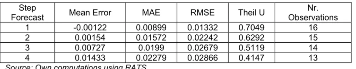
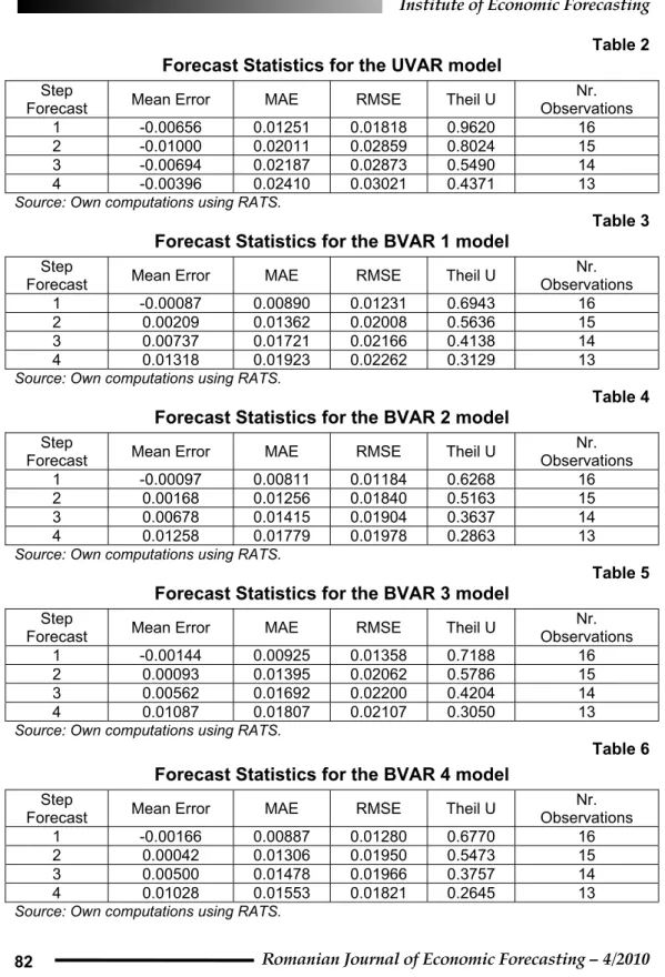
The tables below, Table 1 to Table 6, show the results in terms of quality of forecasting of the output. Clearly, when looking at the Theil U statistics, we see that all models outperform the naïve forecast. We also notice that the four different versions of BVAR models outperform the two standard classical models, OLS or BVAR. When comparing the four versions of BVAR models, based on the RMSE and the Theil U statistics, we see that version 2 and version 4 of the BVAR models are the best. I use the 2nd version of the BVAR model which has the best statistics in terms of RMSE and Theil U statistics.

We can also see that the value of the general tightness parameter, Ȗ, proved to be one of the key elements for the accuracy of forecasts. On one hand, setting the general tightness too high, Ȗ=2 for simple OLS and unstructural VAR, led to a poorer performance. On the other hand, choosing too low a value for this parameter, did not improve the performance, see the cases of Ȗ=0.1. From an economic point of view, the results suggests that the presence of prior information (which can come from different sources, either experience, or economic theory) can significantly improve the forecasts of economic models.

Another important element that made the difference is the relative tightness para-meter, w, which is related to cross lags in each equation. Setting this parameter to almost zero, as for the OLS case, did not prove to be the best option. At the same time, increasing too much this parameter, as w=2.0 for the unrestricted VAR, proved not to be optimal either. The choice of a middle value for the BVAR models, with

w=0.5, produced the best results. Again, there are some economic implications in this

result. Since the w parameter signifies the interactions among the endogenous varia-bles, this imply that the best results in forecasting output are obtained using model-based approaches that take into account the dynamics of other macroeconomic variables (like inflation, investments or interest rates). At the same time, this interaction should not be too much emphasized either, as own shocks (to output, in this case) matter more.

Table 1 Forecast Statistics for the OLS model

Step

Forecast Mean Error MAE RMSE Theil U

Nr. Observations 1 -0.00122 0.00899 0.01332 0.7049 16 2 0.00154 0.01572 0.02242 0.6292 15 3 0.00727 0.0199 0.02679 0.5119 14 4 0.01433 0.02279 0.02866 0.4147 13

(7)

Table 2 Forecast Statistics for the UVAR model

Step

Nr. Observations 1 -0.00656 0.01251 0.01818 0.9620 16 2 -0.01000 0.02011 0.02859 0.8024 15 3 -0.00694 0.02187 0.02873 0.5490 14 4 -0.00396 0.02410 0.03021 0.4371 13

Source: Own computations using RATS.

Table 3 Forecast Statistics for the BVAR 1 model

Step

Nr. Observations 1 -0.00087 0.00890 0.01231 0.6943 16 2 0.00209 0.01362 0.02008 0.5636 15 3 0.00737 0.01721 0.02166 0.4138 14 4 0.01318 0.01923 0.02262 0.3129 13

Step

Nr. Observations 1 -0.00097 0.00811 0.01184 0.6268 16 2 0.00168 0.01256 0.01840 0.5163 15 3 0.00678 0.01415 0.01904 0.3637 14 4 0.01258 0.01779 0.01978 0.2863 13

Step

Nr. Observations 1 -0.00144 0.00925 0.01358 0.7188 16 2 0.00093 0.01395 0.02062 0.5786 15 3 0.00562 0.01692 0.02200 0.4204 14 4 0.01087 0.01807 0.02107 0.3050 13

Step

Nr. Observations 1 -0.00166 0.00887 0.01280 0.6770 16 2 0.00042 0.01306 0.01950 0.5473 15 3 0.00500 0.01478 0.01966 0.3757 14 4 0.01028 0.01553 0.01821 0.2645 13

(8)

4 . Forecasting GDP in the short run

In this section I use the best version of the proposed BVAR models in order to forecast the dynamics of quarterly GDP in the short run.

Figure 1 shows the dynamics of GDP for the period between 2005 and 2009 and the projected GDP from 2009 Q4 to 2010 Q4. What is evident is the acceleration in growth in late 2007 and along 2008 that proved unsustainable. The economic crisis pushed back the GDP at the level of middle 2007. The projection implies a steady tendency of growth, but at a much lower speed that in the last part of economic growth.

It is probable that the economy might return to higher growth rates in the medium run, but at least of the beginning of the recovery, the growth process will be gradual.

Figure 1 Forecasting quarterly GDP for 2009Q4-2010Q4

10.15 10.20 10.25 10.30 10.35 10.40 10.45 2005 2006 2007 2008 2009 2010 Log_Y Log_Y_forecast

Source: Own computations.

In Figure 2, I compare the whole GDP series, including the forecasts of the best BVAR model, with Hodrick-Prescott filtered series (the filter is also applied to the projected values). It appears that the last quarters of growth during the past boom are an anomaly when compared to the trend of output. At the same time, even if the economy starts to grow, the recovery is gradual and, moreover, the output gap will continue to remain, at least initially, in the negative range of values.

(9)

Figure 2 Forecasted GDP and Filtered GDP

10.15 10.20 10.25 10.30 10.35 10.40 10.45 2005 2006 2007 2008 2009 2010 Log_Y Log_Y_HP_filtered

Source: Own computations.

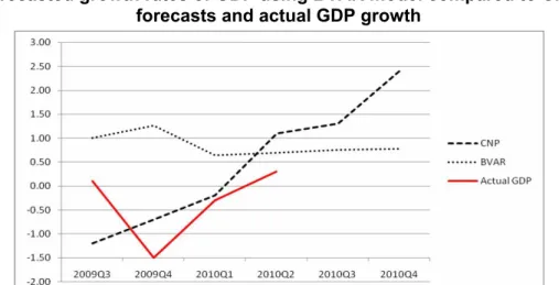
Figure 3 Forecasted growth rates of GDP using BVAR model compared to CNP

forecasts and actual GDP growth

*CNP = National Commission for Forecasting. Source: Own computations.

(10)

In Figure 3, I compare the forecasts provided by the BVAR model with the official forecasts from the National Commission for Forecasting (2009) (CNP hereafter). The data in the figure refer to growth rates relative to the previous quarter. Moreover the figure includes also the actual GDP for Quarter 3 2009 to Quarter 2 2010. The CNP forecast suggested that the lowest point of the crisis was reached in Q4 2009, after which a steady recovery followed. Thus, according to CNP, the recession was supposed to finish in the first quarter of 2010. According, however, to the BVAR forecasts, the recession would finish in the second quarter of 2010. A second difference is related to the speed of recovery. While the CNP forecast indicates a rapid recovery, in the BVAR model, the forecast (as shown also in Figure 2) is slower. When we look at the actual GDP figures we could see that CNP forecasts are much better with respect to the last two quarters of 2009. However, it remains to be seen in the following quarters if the recovery will be fast or if the recovery will slow-down. A third possibility which is not however forecasted in any of the two approaches is that of a W-shape recovery, in which the economy will undergo a second smaller recession. As Gupta and Sichei (2007) underscored, this approach, although it performed very well, had severely important limitations. Among these, one can underline that it is influenced by the presence or absence of structural breaks which can distort estimation as well as the quality of forecasts. Second of all, such an approach is not linear by nature and thus can be rendered as inappropriate during severe economic crises which might imply nonlinear features or switching phenomena. Third of all, such an approach could be improved through the newest DSGE paradigm which provides a structural approach and is proved to provide better forecasts (several papers also proposed the so-called DSGE-BVAR approach).

C

onclusion

Following the economic crisis, many people from diverse positions raised questions about the ability of the economists to accurately predict the future, as the Great Recession was unpredicted by most of the economists. This is why the challenge for economists to build better and better models for forecasting becomes even harder. In this paper I contribute to the ongoing expansion of using Bayesian methods to forecast the economic activity. For an economy like Romania’s, where data are not available for longer periods and where there are frequent structural changes, the Bayesian approach could provide a competitive alternative approach.

By using the Bayesian VAR framework, I estimated several BVAR models which I compared in terms of forecasting accuracy with two standard models, the OLS and the UVAR, as well as with a “naïve forecast”. The results show that the BVAR approach clearly outperforms the other approaches, confirming the general findings in the literature.

The best BVAR model in terms of forecasting was used to forecast the dynamics of quarterly GDP for five quarters, until Q 4 2010. The results show that the recovery will be slow and gradual and that the output gap will continue to be negative in the short run.

(11)

The findings in this paper suggest that the BVAR approach should be further used for the Romanian economy. Some more complex models could include an extension to the open economy case or constructing models to analyze monetary and fiscal policy.

R

eferences

Artis, M.J., and W. Zhang, (1990), “BVAR Forecasts for the G7.” International Journal

of Forecasting, 6: 349-362.

Caraiani, P. (2009), “Forecasting the Romanian GDP in the Long Run Using a Monetary DSGE”, Romanian Journal for Economic Forecasting, 11(3): 75-84.

Ciccarelli, M. and A. Rebucci. (2003), “Bayesian VARs: A Survey of the Recent Literature with an Application to the European Monetary System”,IMF

Working Papers 03/102, International Monetary Fund.

Doan. 2007. RATS User’s Manual version 7, Estima.

Doan, Th., R. Litterman, and Ch. Sims, (1984), “Forecasting and conditional projection using realistic prior distributions”, Econometric Reviews, 3(1):1-100. Dobrescu, E. (2006), “Macromodels of the Romanian Market Economy”,. Bucharest:

Editura Economica,.

Dua, P. and S.M. Miller. (1996), “Forecasting and Analyzing Economic Activity with Coincident and Leading Indexes: The Case of Connecticut”, Journal

of Forecasting, 15: 509-526.

Dua, P., S.M. Miller and D.J. Smyth. (1999), “Using Leading Indicators to Forecast US Home Sales in a Bayesian Vector Autoregression Framework”,

Journal of Real Estate Finance and Economics, 18: 191-205.

Gupta, R. and M. Sichei, (2006), “A BVAR Model For The South African Economy”,

South African Journal of Economics, 74(3): 391-409.

Gupta, R. (2007), “Forecasting the South African Economy with Gibbs sampled BVECMS”,South African Journal of Economics, 75(4): 631-643. Kadiyala, K. and S. Karlsson. (1997), “Numerical Methods for Estimation and

Inference in Bayesian VAR Models”, Journal of Applied Econometrics, 12: 99-132.

Kenny, G., A. Meyler, and T. Quinn. (1998), “Bayesian VAR Models for Forecasting Irish Inflation”, MPRA Paper 11360, University Library of Munich, Germany.

Litterman , R. (1980), “Techniques for Forecasting with Vector Autoregressions”, University of Minnesota, Ph.D. Dissertation.

Litterman, R. (1986), “Forecasting with Bayesian Vector Autoregressions: Five Years of Experience”, Journal of Business and Economic Statistics, 4(1): 25-38.

Lucas, R. Jr. (1976), ”Econometric policy evaluation: A critique”, Carnegie-Rochester

Conference Series on Public Policy, 1(1): 19-46.

National Commission for Forecasting. (2009), “The Projection of the Main Macroeconomic Indicators for the 2009-2014 period”, The 2009 Fall

(12)

Poirier, D. (2008), “Bayesian Econometrics”, In S.N. Durlauf and L.E. Blume (eds),

The New Palgrave Dictionary of Economics, Palgrave Macmillan.

Sims, C. (1980), “Macroeconomics and reality”, Econometrica, 48: 1-48.

Sims, C. (2007), “Bayesian Methods in Applied Econometrics, or, Why Econometrics Should Always and Everywhere Be Bayesian”, Hotelling lecture, June 29, 2007, Duke University.

Schorfheide, F. (2008), “Bayesian Methods in Macroeconometrics”, In S.N. Durlauf and L.E. Blume (eds), The New Palgrave Dictionary of Economics, Palgrave Macmillan.

Theil, H. (1963), “On the Use of Incomplete Prior Information in Regression Analysis”,

Journal of the American Statistical Association, 58: 401-414.

Annex A: Lag Length Criteria Test VAR Lag Order Selection Criteria

Endogenous variables: LOG_INV LOG_PI LOG_R LOG_Y

Exogenous variables: C Sample: 1999Q1 2010Q4 Included observations: 39

Lag LogL LR FPE AIC SC HQ

0 91.63895 NA 1.31e-07 -4.494305 -4.323683 -4.433088

1 317.5969 393.9780 2.78e-12 -15.26138 -14.40827 -14.95529

2 347.9033 46.62525* 1.37e-12* -15.99504* -14.45945* -15.44408*

3 362.6700 19.68887 1.57e-12 -15.93179 -13.71371 -15.13596

4 374.4552 13.29620 2.26e-12 -15.71565 -12.81508 -14.67495

* indicates lag order selected by the criterion