How good are dynamic factor models at forecasting output and inflation? A meta-analytic approach

How good are dynamic factor models

at forecasting output and inflation?

A meta-analytic approach

Sandra Eickmeier

(Deutsche Bundesbank and University of Cologne)

Christina Ziegler

(University of Bonn)

Discussion Paper

Series 1: Economic Studies

No 42/2006

Editorial Board: Heinz Herrmann

Thilo Liebig

Karl-Heinz Tödter

Deutsche Bundesbank, Wilhelm-Epstein-Strasse 14, 60431 Frankfurt am Main, Postfach 10 06 02, 60006 Frankfurt am Main

Tel +49 69 9566-1

Telex within Germany 41227, telex from abroad 414431 Please address all orders in writing to: Deutsche Bundesbank,

Press and Public Relations Division, at the above address or via fax +49 69 9566-3077

Internet http://www.bundesbank.de

Reproduction permitted only if source is stated. ISBN 3–86558–235–4 (Printversion) ISBN 3–86558–236–2 (Internetversion)

Abstract:

This paper surveys existing factor forecast applications for real economic activity and inflation by means of a meta-analysis and contributes to the current debate on the determinants of the forecast performance of large-scale dynamic factor models relative to other models. We find that, on average, factor forecasts are slightly better than other models’ forecasts. In particular, factor models tend to outperform small-scale models, whereas they perform slightly worse than alternative methods which are also able to exploit large datasets. Our results further suggest that factor forecasts are better for US than for UK macroeconomic variables, and that they are better for US than for euro-area output; however, there are no significant differences between the relative factor forecast performance for US and euro-area inflation. There is also some evidence that factor models are better suited to predict output at shorter forecast horizons than at longer horizons. These findings all relate to the forecasting environment (which cannot be influenced by the forecasters). Among the variables capturing the forecasting design (which can, by contrast, be influenced by the forecasters), the size of the dataset from which factors are extracted seems to positively affect the relative factor forecast performance. There is some evidence that quarterly data lend themselves better to factor forecasts than monthly data. Rolling forecasts are preferable to recursive forecasts. The factor estimation technique seems to matter as well. Other potential determinants - namely whether forecasters rely on a balanced or an unbalanced panel, whether restrictions implied by the factor structure are imposed in the forecasting equation or not and whether an iterated or a direct multi-step forecast is made - are found to be rather irrelevant. Moreover, we find no evidence that pre-selecting the variables to be included in the panel from which factors are extracted helped to improve factor forecasts in the past.

JEL: C2, C3, E37

Non-Technical Summary

In recent times, dynamic factor models are increasingly applied in central banks to forecast economic developments based on large datasets. This paper adopts a meta-analytic approach to evaluate the forecast performance of these models relative to other models for real economic activity and inflation. This approach allows us to systematically summarize findings from existing factor forecast applications using statistic and econometric techniques. At the same time, we are able to assess the relevance of a large number of determinants which are able to influence the forecast performance.

Based on more than 45,000 observations taken from 46 studies, we find that, on average, factor forecasts perform slightly better than other models’ forecasts, with inflation forecasts having some advantages over output forecasts. However, this also involves a greater dispersion of results associated with inflation.

The main findings regarding the determinants are the following. The size of the dataset from which factors are extracted seems to positively affect the relative factor forecast performance. Recursive factor forecasts are inferior to rolling factor forecasts, which are able to better account for possible structural breaks in the factors. Moreover, it seems to matter which factor estimation technique is applied. According to our analysis, the dynamic approaches proposed by Forni et al. (2005) and Kapetanios and Marcellino (2004) tend to outperform the static approach of Stock and Watson (2002), which, however, is much easier to implement. Our results further suggest that factor models have some advantages when predicting US compared to UK macroeconomic variables. Factor models also seem to be better suited to forecasting US output than euro-area output, but there are no significant differences between the relative factor forecast performance for US and euro-area inflation. Factor models perform slightly worse than alternative methods which are also able to exploit large datasets, but they generally outperform small-scale models. There is some evidence that quarterly data are better suited to factor forecasts than monthly data and that the relative factor forecast performance worsens with the forecast horizon for output, whereas the forecast horizon does not seem to matter for inflation. Other potential determinants, namely whether forecasters rely on a balanced or an unbalanced panel, whether restrictions implied by the factor structure are imposed in the forecasting equation or whether this equation is estimated unrestrictedly and whether an iterated or a direct multi-step forecast is made, are found to be rather irrelevant. Moreover, we find no evidence that pre-selecting the variables to be included in the panel from which factors are extracted helps to improve factor forecasts.

Our analysis can help practitioners to improve their forecasts. Our main messages are the following. First, it seems worthwhile exploiting large datasets. Second, it is important to carefully specify the forecasting model. Although more demanding in terms of specification, complex factor estimation techniques tend to perform relatively well and restricted estimation of the forecasting equation does not seem to be inferior to unrestricted estimation. Third,

some potential determinants were found to be surprisingly irrelevant in the empirical analysis, given that researchers have paid relatively much attention to them in the past. This refers, for instance, to whether the data have been selected prior to the factor estimation, whether or not restrictions implied by the factor structure are imposed in the forecasting equation and whether an unbalanced or a balanced panel is used. Another determinant, by contrast, turns out to be surprisingly important and robust, given that it has not attracted much attention in the existing literature to date: whether the forecast is made based on a rolling or a recursive window.

Nicht technische Zusammenfassung

Dynamische Faktormodelle werden in der letzter Zeit verstärkt von Zentralbanken angewandt, um volkswirtschaftliche Entwicklungen auf Basis umfangreicher Datensätze vorherzusagen. Der vorliegende Artikel untersucht mit Hilfe einer Meta-Analyse die Fähigkeit solcher Modelle zur Prognose von realwirtschaftlicher Aktivität und Inflation relativ zur Prognosefähigkeit alternativer Modelle. Dieser Ansatz erlaubt es, auf Basis statistischer und ökonometrischer Methoden einen systematischen Überblick über existierende Anwendungen zur Prognose mit Faktormodellen zu geben. Gleichzeitig kann die Bedeutung einer großen Anzahl möglicher Determinanten untersucht werden, welche die Prognosegüte beeinflussen können.

Auf Basis von über 45,000 Beobachtungen, die aus 46 Studien entnommen wurden, finden wir, dass im Durchschnitt Faktormodelle leicht besser prognostizieren als andere Modelle, mit gewissen Vorteilen bei der Inflationsprognose gegenüber der Prognose der realwirtschaftlichen Aktivität; allerdings streuen die Ergebnisse bei der Inflationsprognose auch stärker.

Die wichtigsten Ergebnisse bezüglich der Determinanten lassen sich wie folgt zusammenfassen. Die Größe des Datensatzes, auf dessen Basis die Faktoren geschätzt werden, scheint sich positiv auf die relative Prognosefähigkeit von Faktormodellen auszuwirken. Rekursive Faktorprognosen sind rollierenden Faktorprognosen, die mögliche Strukturbrüche in den Faktoren besser berücksichtigen können, unterlegen. Des Weiteren scheint es eine Rolle zu spielen, welche Technik zur Schätzung der Faktoren angewandt wird. So schneiden die dynamische Schätzmethoden von Forni et al. (2005) und von Kapetanios und Marcellino (2004) in unserer Analyse besser ab als der von Stock und Watson (2002) vorgeschlagene statische Ansatz, welcher allerdings den Vorteil hat, dass er leichter zu implementieren ist. Unsere Ergebnisse legen zudem nahe, dass Faktormodelle Vorteile bei der Prognose US-amerikanischer makroökonomischer Variablen haben im Vergleich zur Prognose britischer Variablen. Faktormodelle scheinen zudem besser geeignet, Output in den Vereinigten Staaten als Output im Euro-Raum vorherzusagen, wohingegen sich die Befunde zur Inflationsprognose in beiden Gebieten nicht signifikant voneinander unterscheiden. Wir finden weiter, dass mit Faktormodellen leicht schlechter prognostiziert wird als mit alternativen Methoden, welche ebenfalls in der Lage sind, große Datensätze zu nutzen; dagegen schneiden Faktormodelle in der Regel besser ab als kleine Prognosemodelle. Zudem gibt es Evidenz dafür, dass die Prognose mit Faktormodellen relativ zu anderen Modellen besser ist, wenn sie auf Basis vierteljährlicher als auf Basis monatlicher Daten vorgenommen wird. Weiterhin deuten unsere Ergebnisse darauf hin, dass sich die relative Fähigkeit von Faktormodellen, Output vorherzusagen, mit zunehmendem Prognosehorizont verschlechtert; hingegen scheint der Prognosehorizont keinen Einfluss auf die relative

Faktorprognosefähigkeit von Inflation zu haben. Andere mögliche Bestimmungsgrößen sind eher irrelevant, etwa ob Prognostiker Faktoren auf Basis eines balancierten oder eines unbalancierten Panel schätzen, ob Restriktionen, die durch die Faktorstruktur impliziert werden, auch in der Prognosegleichung auferlegt werden oder ob jene unrestringiert geschätzt wird und ob iterative oder direkte Mehrschrittprognosen durchgeführt werden. Schließlich finden wir keine Anhaltspunkte dafür, dass eine Vorauswahl der Variablen, die in den Datensatz eingehen, aus dem die Faktoren extrahiert werden, eine Verbesserung der relative Prognosefähigkeit von Faktormodellen bewirkt.

Unsere Analyse kann angewandten Prognostikern helfen, ihre Vorhersage zu verbessern. Unsere wichtigsten Botschaften sind die folgenden. Erstens scheint es sich zu lohnen, Informationen aus großen Datensätzen auszunutzen. Zweitens sollte das Prognosemodell sorgfältig spezifiziert werden. Zwar stellen komplexere Faktorschätztechniken höhere Anforderungen an die Prognostiker im Hinblick auf die Spezifikation, sie schneiden tendenziell aber besser ab, und auch die restringierte Schätzung der Prognosegleichung ist der unrestringierten nicht unterlegen. Drittens deuten unsere Untersuchungen darauf hin, dass einige möglichen Bestimmungsgründe der relativen Prognosefähigkeit von Faktormodellen überraschend irrelevant sind, angesichts der Tatsache, dass Forscher Ihnen in der Vergangenheit relativ viel Aufmerksamkeit beigemessen haben. Dies bezieht sich zum Beispiel darauf, ob und inwiefern vor der Faktorschätzung eine Auswahl der Variablen getroffen, ob durch die Faktorstruktur implizierte Restriktionen auch in der Prognosegleichung berücksichtigt und ob auf ein balanciertes oder ein unbalanciertes Panel abgestellt werden soll. Dagegen hat sich eine andere Bestimmungsgröße als bedeutend und robust herausgestellt, nämlich ob rollierend oder rekursiv prognostiziert wird. Dies ist erstaunlich, da ihr bislang wenig Beachtung geschenkt wurde.

Contents

1 Introduction 1

2 Forecasting with dynamic factor models 3

2.1. A two-step forecasting approach 4

2.2. Determinants of factor forecasts 5

3. Preparing the meta-analysis 12

3.1. Collecting relevant papers 12

3.2. Meta-dependent variable 12 3.3. Meta-independent variables 13 4. Results 17 4.1. Descriptive analysis 17 4.2. Meta-regression 18 4.2.1. Baseline meta-regression 18

4.2.2. Robustness checks: outliers, sampling bias, dependency

and qualitative differences 21

5. Conclusion 24

Tables and Figures

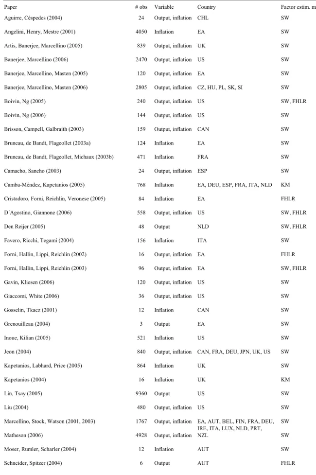
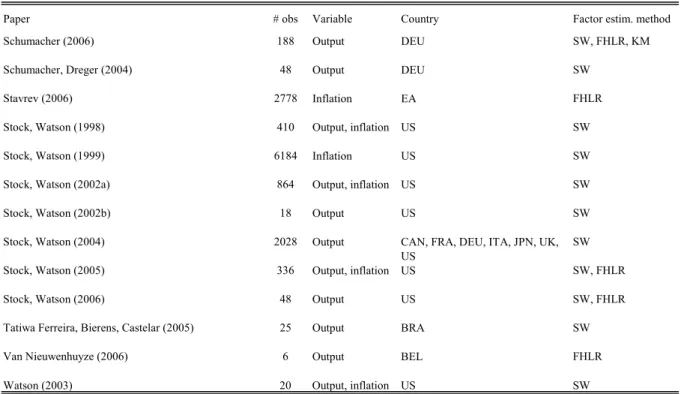
Table 1 Studies included in the meta-analysis 26

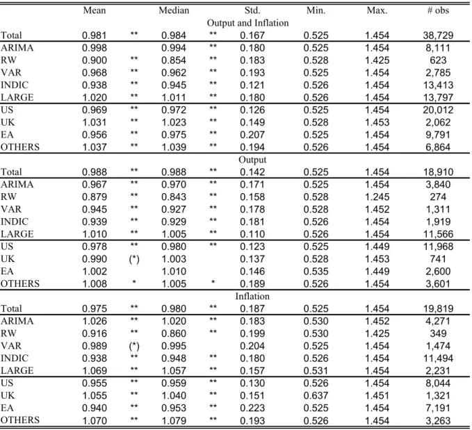
Table 2 Descriptive statistics 28

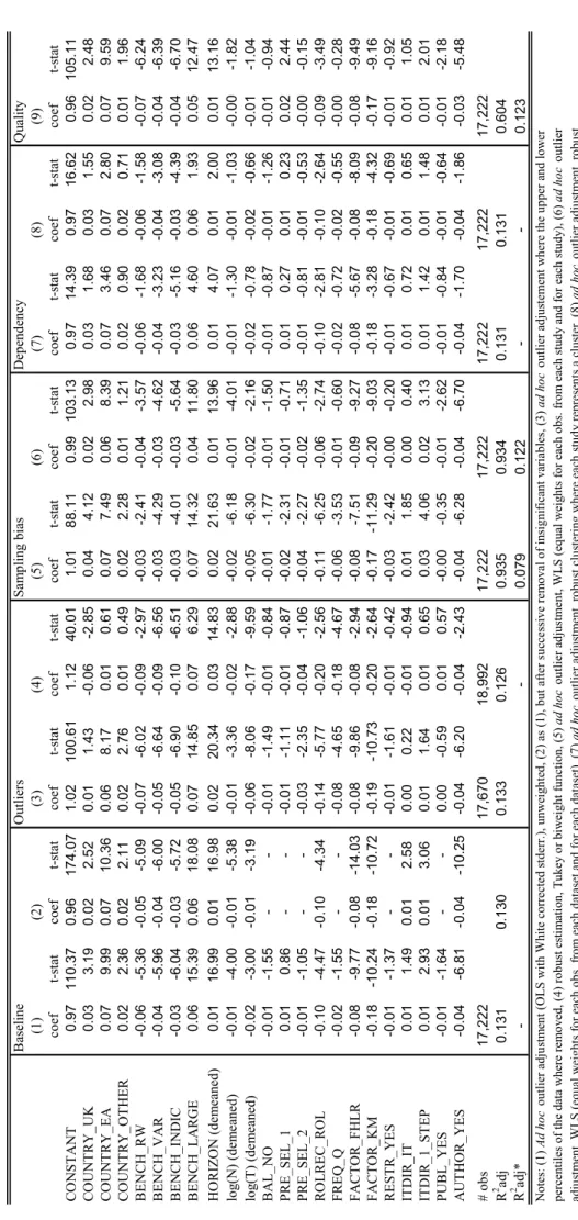
Table 3 Meta-regression results for output 29

Table 4 Meta-regression results for inflation 30

How Good are Dynamic Factor Models at Forecasting

Output and Inflation? A Meta-Analytic Approach

*

1. Introduction

Large-dimensional dynamic factor models are being increasingly applied by policymakers and economic research institutions to forecast key macroeconomic variables, such as real output and inflation. This is partly because many time series are nowadays readily available, and modern computers and software allow us to efficiently summarize the information contained in large datasets. The use of dynamic factor models has been further improved by recent advances in estimation techniques proposed by Stock and Watson (2002a; henceforth SW), Forni, Hallin, Lippi and Reichlin (2005; henceforth FHLR) and Kapetanios and Marcellino (2004; henceforth KM). The two former approaches rely on static and dynamic principal component analysis (PCA), respectively, and the latter on a subspace algorithm. These techniques allow forecasters to easily summarize the information contained in large datasets and extract a few common factors from them. All or a subset of the estimated factors are then entered into rather simple regression models to predict key macroeconomic variables. Exploiting information from large panels, normally, should help to improve forecasts, and early results were very promising in this respect (cf. SW, FHLR). However, more recent applications find no or only minor improvements (cf. Schumacher 2006; Schumacher and Dreger 2004; Gosselin and Tkacz 2001; Banerjee et al. 2004; Angelini et al. 2001). These conflicting results have launched a lively discussion on whether large-scale factor models are really as useful for forecasting practice as first expected. Some researchers speculate about the conditions under which factor models perform well in forecasting. Banerjee et al. (2005), for example, claim that factor models are relatively good at forecasting real variables in the US but less so in the euro area, whereas, according to the authors of this paper, euro-area nominal variables are easier to predict using factor models than US nominal variables. Likewise, Boivin and Ng (2006) have argued that the composition of the dataset, and not only the pure size of the cross-section dimension, is crucial to producing passable forecasts with factor models. Another debated issue is which of the factor estimation techniques performs best. As will be explained in detail below, the dynamic approaches of FHLR and KM are potentially more efficient than the static SW approach, but also more prone to misspecification.

* _{Affiliations: Sandra Eickmeier, Deutsche Bundesbank, Wilhelm-Epstein-Straße 14, D – 60431 Frankfurt am} Main and University of Cologne, [email protected]; Christina Ziegler, University of Bonn (and visitor of the Deutsche Bundesbank while working on this project), [email protected].

We are grateful to Jörg Breitung, Ben Craig, Ard den Reijer, Heinz Herrmann, Robinson Kruse, Christian Offermanns and Christian Schumacher for their helpful comments and for the discussions. This paper was presented at a seminar at the Deutsche Bundesbank and at macroeconometric workshops in Berlin and Halle.

The motivation for our paper is twofold. First, a considerable number of papers have been written now, and forecasters from policy institutions are on the verge of integrating factor models into the regular forecasting process. We therefore believe that it is time to systematically summarize this literature. Second, our paper is an attempt to contribute to the discussion on the determinants of the relative forecast performance of factor models. It is

unclear a priori how some of the potential determinants affect the factor forecast

performance, but this question needs to be solved empirically. Our paper tries to identify the relevant determinants and to indicate ways in which factor model forecasts can be improved further.

Our paper surveys studies which have predicted real economic activity and inflation using large-scale dynamic factor models. We summarize the papers’ findings and assess which potential determinants of the relative factor forecast performance have been relevant in existing empirical applications. For this purpose, we carry out a meta-analysis. Meta-analyses were first applied in health, educational and psychological sciences for some time, and recently became popular also in macroeconomics (cf. Stanley 2001 and articles in the special edition of the Journal of Economic Surveys 2005, Vol. 19(3) and Weichselbaumer and Winter-Ebmer 2005, which, in methodological respects, is closely related to our analysis). They are powerful tools to systematically summarize previous studies’ findings, based on formal statistical and econometric techniques, and to detect their determinants. The idea is to collect existing studies which are on a certain issue to be studied, take statistics of interest from these studies, look at empirical distributions and regress these statistics on a number of determining characteristics. Our statistic of interest (or meta-dependent variable) measures the relative factor forecast performance, and we take the root mean squared error (RMSE) of a forecast based on a large-scale dynamic factor model relative to the RMSE of a forecast based on a benchmark model. Overall, we collect 45,111 statistics (or converted related statistics into relative RMSEs, if necessary) out of a total of 46 studies. We provide some descriptive statistics and test in particular, whether factor model forecasts are significantly better or worse compared to other models’ forecasts. Theory gives us some guidance on possible determinants of the factor forecast performance. We record these determinants for each observation and regress relative RMSEs on them to examine which forecast environments and designs lend themselves to factor forecasts – and which do not.

Our paper is related to other papers surveying (among others) factor forecast applications such as Reichlin (2003), Stock and Watson (2006) and Breitung and Eickmeier (2006). Those papers all adopt a narrative approach which is more prone to the subjectivity regarding the choice of papers and results. Our paper is also related to a literature which concentrates on certain aspects of factor forecasting in an otherwise broad context. Examples are Kapetanios and Marcellino (2004) and Schumacher (2006) who explicitly compare factor estimation techniques; Boivin and Ng (2005) and D’Agostino and Giannone (2006), who also concentrate on the implementation of estimated factors in the forecasting equation; and

Boivin and Ng (2006), among others, who look at the variables included in the dataset from which the factors are extracted. The advantage of our meta-analytic approach is that many possible determinants, and not just a few, can be considered simultaneously. It has a very broad scope, which allows us to reconcile and explain differences in findings across individual studies.

The results of our analysis can be summarized as follows. On average, factor forecasts are slightly better than other models’ forecasts. In particular, factor models tend to outperform small-scale models, whereas they perform slightly worse than alternative methods which are also able to exploit large datasets. Our results further suggest that factor forecasts are better for US than for UK macroeconomic variables, and that they are better for US than for euro-area output; however, there are no significant differences between the relative factor forecast performance for US and euro-area inflation. There is also some evidence that factor models are better suited to predict output at shorter forecast horizons than at longer horizons. These findings all relate to the forecasting environment (which cannot be influenced by the forecasters). Among the variables capturing the forecasting design (which can, by contrast, be influenced by the forecasters), the size of the dataset from which factors are extracted seems to positively affect the relative factor forecast performance. There is some evidence that quarterly data lend themselves better to factor forecasts than monthly data. Rolling forecasts are preferable to recursive forecasts. The factor estimation technique seems to matter as well. Other potential determinants - namely whether forecasters rely on a balanced or an unbalanced panel, whether restrictions implied by the factor structure are imposed in the forecasting equation or not and whether an iterated or a direct multi-step forecast is made - are found to be rather irrelevant. Moreover, we find no evidence that pre-selecting the variables to be included in the panel from which factors are extracted helped to improve factor forecasts in the past.

Our paper is organized as follows. Section 2 presents the approximate dynamic factor model and explains how it is used for forecasting in macroeconomics. It further discusses determinants of factor forecast performance. Section 3 describes the preparatory work in the run-up to the meta-analysis including the collection of relevant papers and the construction of the dataset. Section 4 presents some descriptive statistics, the meta-analytic design and the results. Section 5 concludes.

2.

Forecasting with dynamic factor models

We consider a situation where a forecaster is interested in predicting a certain macroeconomic (target) variable y_t. He/she may do this by fitting small-scale time series models such as AR models, which exploit the dynamics of the target variable itself, or VAR models, which, in addition, account for interdependencies among a few variables, to y_t. These simple models have performed fairly well in the past. Nowadays, however, lots of data are available to

forecasters. Those data may contain information which is useful to predict y_t. As has been shown by numerous studies, economic variables strongly comove, and some variables are leading and may provide useful signals for others.

It is, however, not feasible to include all potentially relevant variables simultaneously in a forecasting equation. And this is where factor models come into play. The idea underlying factor models is that the bulk of variation of many variables can be explained by a small number of common factors or shocks. This idea dates back to Burns and Mitchell (1946), and, for instance, Giannone et al. (2004) and Uhlig (2004) have shown empirically that economies are driven by a few factors or shocks. Factor models exploit the variables’ comovement and efficiently reduce, in a first step, the dimension of the dataset to just a few underlying factors. In a second step, these factors are included into a rather small forecasting equation to predict

t

y , and only a few parameters need to be estimated. Let us explain these two steps in some detail.

2.1. A two-step forecasting approach

This subsection presents the approximate dynamic factor model and how it is used to make forecasts. It is assumed that a large number of variables x_it, i=1,...,N, collected in

[

]

'

1t ... it ... Nt

t = x x x

X , are driven by few (q<<N) unobserved common factors,

summarized in f_t =

[

f_1t ... f_qt

]

'. Accordingly, dynamic factor models express the time series

it

x as the sum of a common component _χit and an idiosyncratic component _ξit. The common component is the product of the q×1 vectors of dynamic factors which are common to all

variables in the set, f_t, (and possibly their lags) and the factor loadings

s is i i i L λ λ L λ L λ ( )= ₀ + ₁ +...+ : it t i it it it L x =_χ +_ξ =_λ ( )'f +_ξ . (1)

It is useful to write down the static representation of the model:

it t i it

x =Λ 'F +_ξ , (2)

where F_t is a vector of r ≥q static factors that comprises the dynamic factors f_t and all lags of the factors which enter with at least one non-zero weight in the factor representation. The

1

×

r vector Λ_i comprises all non-zero columns of (_λi0,...,_λis). The factors are orthogonal to each other. It is assumed that the factors follow a VAR(_pF_{) process and that the idiosyncratic}

components are weakly serially and cross-correlated in the sense of Bai and Ng (2002). For forecasting purposes, it is also useful to represent the idiosyncratic errors as AR(pξ) processes (cf. Boivin and Ng 2005)

it it i t t =u , (1−ρ (L))ξ =υ A(L))F -(I , (3) where F F p p L L L L A A A A( )= + 2 +...+ 2 1 and ξ ξ ρ ρ ρ ρ p ip i i i(L)= 1L+ 2L2 +...+ L .

In the literature, there exist basically three methods of estimating the factors F_t from a large dataset, namely those developed by SW, FHLR and KM. We will explain the different estimation methods in detail below, but let us, for the moment, simply assume that Fˆ_t denotes the vector of estimated factors by one of the three methods.1

In a second step, the estimated factors or a subset thereof – let us denote them by the r×1

vector Fˆ – are included in a forecasting equation to predict _t y_t which may or may not be included in X_t.2 The equation is usually given by

h t t t h t L L y y₊ =α₀ +α₁( )'Fˆ +α₂( )' +ε ₊ , (4)

where h is the forecast horizon, ( )

(

2 ...

)

,

{ }

1,2

2 1 0 + + + + = = L L L i L i i p ip i i i i α α α α α α α are r

-dimensional (i =1) and scalar (i=2) lag polynomials and _αi(L) can be estimated unrestrictedly or restrictedly. Forecasts are evaluated based on forecast error losses, and forecast error losses obtained from factor model forecasts are then compared with forecast error losses obtained from some benchmark models.

Papers using dynamic factor models to predict macroeconomic variables differ in various respects and, not surprisingly, come to different conclusions regarding the relative forecasting performance of factor models. Theory provides some guidance as to which conditions and what forecast design should lead to good outcomes.

2.2. Determinants of factor forecasts

If the factors and parameters were known and the target variable was correlated with the factors, factor models should deliver smaller forecast errors compared to AR models. This is nicely illustrated in Boivin and Ng (2005) and - to make our paper self-contained - we roughly repeat their illustration in the following paragraph.

Let us suppose for the moment that the variable we want to predict is x_it+1 and is, thus, contained in X_t, and – for simplicity – that r =1 and the factor and the idiosyncratic component follow AR processes of order 1. Iterating equation (2) one period forward and plugging in expressions for F_t+1 and _ξit+1, we obtain

1 1 1 '( + ) + + =Λi t + t + i it + it it x AF u _{ρξ υ} . (5)

1 _{Here and in the following, a ‘^’ stands for an estimate.} 2 _{It may be that}

t

t F

Fˆ =ˆ , i.e. that the factors underlying X_tare identical to the factors included in the forecasting equation. However, some papers include Fˆ_t ≠Fˆ_t in the forecasting equation, where Fˆt is a subset of Fˆt (in this

Solving (2) for _ξit and plugging this expression into (5) yields 1 1 1 '( ' + + + = i it +Λi i t +Λi t + it it x x _ρ A-_ρ )F u _υ . (6)

From (6), it is apparent that AR(1) forecasts can be regarded as a special case (for Λi =0) of factor forecasts. Moreover, factor forecasts deliver smaller mean squared errors than AR(1) models as long as the factors and parameters are known, the target variable is correlated with the factors, i.e. Λi ≠0, and the factors and idiosyncratic components have different dynamics, i.e. A≠ _ρi.

While the latter condition is generally fulfilled in practice, this does not hold for the other conditions. Factors are unknown. They need to be estimated and the factor estimates, not the true factors are included in the forecasting equation. Moreover, the target variable is not necessarily correlated with the factors included in the forecast equation, and introducing uninformative factors in the forecast equation would only increase sampling variability. Finally, researchers do not know the models’ parameters and are not immune to misspecifications in the forecasting equations.

Whether forecasters face these problems, will depend on the specific forecasting environment and the forecasting design. While they generally have to take the former as given, they can choose the factor forecast design and have, in this respect, some influence on the outcomes. In the following, we identify the determinants of the relative factor forecast performance, classify them into determinants capturing the forecast environment (which cannot be influenced by the forecasters) and those affecting the forecast design (which can be influenced by the forecasters) and discuss implication for the precision of factor estimates, the commonality of the target variable and the specification of the forecasting equation.

Forecasting environment (which cannot be influenced by the forecasters)

The degree of commonality obviously differs across variables, with some variables linked more closely to the overall economic development than others. We will below distinguish forecasts of output and inflation in different countries or regions.

In addition, the relative forecast performance of factor models should vary with the benchmark model, with some models accounting more for the commonality of the target variable than others. While univariate models such as random walks and ARIMA models do not consider the cross-variation between the variables at all, other popular benchmarks such as VAR models or single equation models with one or a very few observable indicators do; also, the issue of whether the target variable is related to a stronger extent to the factors or to the observable indicators will govern the relative forecast performance. Recently, alternative models which are able to exploit the data-rich environment, such as forecast combination, model averaging including Bayesian model averaging and bagging, ridge regression,

shrinkage and partial least squares have been proposed (cf. Stock and Watson 2004 and 2006, Lin and Tsay 2005).

Also, the forecast horizon is generally given to the forecasters. Two arguments come to our mind. The greater the predictability of the common component relative to the idiosyncratic component at larger horizons (which is positively related to the relative persistence of the two components), the better the forecast performance of factor models should be relative to small-scale models such as AR models. Moreover, if X_t contains leading indicators of y_t, which is typically the case, we would expect factor models to be more successful than, for instance, univariate models at predicting y_t at longer horizons.

The commonality of the target variable and, hence, the relative forecast performance of factor models could also be altered by the specific estimation period. Variables comove more in certain periods than in others, and we would therefore expect factor models to be better suited for forecasting in periods of greater comovements. It is, for example, well known that variables move relatively closely together during economic downturns. Likewise, periods which are characterized by lower economic volatility, such as the great moderation period since 1985, are less well described by a factor model, as shown by D’Agostino and Giannone (2006). We are not able to capture this effect here, since only very few papers consider periods which are clearly characterized as being periods of either high or low comovement.

Forecasting design (which can be influenced by the forecasters)

Choosing the forecasting design mainly means constructing the dataset from which the factor are extracted and estimating the factors and the forecasting equation.

Regarding the dataset, it is a well-known result of the factor literature that there are benefits from information contained in large datasets in terms of greater precision of the factor estimates. Stock and Watson (2002a) and Bai and Ng (2002), for example, show that the uncertainty associated with the factor estimation becomes negligible and factors can be treated as known if the cross-section dimension of X_t, N, and the number of observations,

T, tend to infinity. This result suggests that the forecast performance of factor models should improve with N and T.

However, various studies demonstrate that it is not the pure size of the dataset,3 but also its characteristics, which matter for forecasting. Forecasters should take care that variables which are highly correlated among each other are included in the dataset; this should improve the precision of the factor estimation. Moreover, the dataset should contain variables which are

3 _{Watson (2003) and Bai and Ng (2002) show in real-time experiments and in simulations that there are basically} no gains from increasing N beyond 50 or 40, respectively. Boivin and Ng (2006) demonstrate that increasing N beyond a certain number can even be harmful and may result in efficiency losses.

highly correlated with the target variable. Forecasters often face a trade-off between including many time series and/or many observations and times series which satisfy these two requirements. This trade-off is reflected in the following determinants.

One issue is whether it is well suited to extract factors from a balanced or an unbalanced panel. Forecasters relying on an unbalanced panel argue that additional information from time series with missing observations can be exploited. Improvements in terms of forecasting performance can, however, only be expected if these additional time series comove with the other variables contained in the panel and/or with the target variable.

Another issue is raised by Boivin and Ng (2006). They show that the inclusion of variables with errors which have large variances and/or are cross-correlated, should worsen the precision of factors estimates. The forecast performance of factor models may also be worsened if variables that are irrelevant for y_t are included in X_t - this is referred to as the oversampling problem. Boivin and Ng (2006) suggest pre-selecting the variables to be included in X_t and removing variables with correlated and/or large errors and/or variables which are irrelevant for the target variable prior to estimating the factors.

A third issue which is relevant in this context is whether to use a recursive or a rolling factor estimation (and forecasting) scheme. A forecast based on a recursive scheme relies on an estimation period of increasing length, where the starting point remains fixed, whereas a rolling scheme relies on a fixed-length window which is shifted every period. A priori, it is unclear which scheme would yield more precise factor estimates. On the one hand, the recursive scheme allows us to exploit more information since estimation tends to be based on a larger T. On the other hand, if factors (and/or factor loadings) are subject to structural breaks which occur in the course of the estimation period, a rolling scheme which gives observations in the past a lower weight compared to a recursive scheme should deliver better forecasts.

A fourth issue regards the frequency. Quarterly times series correspond to averages of the monthly series or smoothed monthly series. If idiosyncratic noise is averaged away, as one might expect, rather than the common part of the variables, commonality will be greater at quarterly than at monthly frequency, although monthly data potentially contain more information.

Besides the size and the composition of the dataset, estimation techniques also matter for factor forecasts. This refers to the factor estimation technique and to the specification and estimation of the forecasting equation.

The technique used to estimate the factors should affect the precision of the estimates. As already pointed out above, basically three different methods are employed in the literature, namely those proposed by SW and FHLR and the more recently developed, still less frequently applied KM method. Let us briefly explain them.

SW propose estimating F_t with static PCA applied to X_t. The factor estimates are simply the first r principal components of X_t, FSW 'X_t

t =Λˆ

ˆ _{, where Λˆ is the N×r matrix of the}

eigenvectors corresponding to the r largest eigenvalues of the sample covariance matrix Σˆ .

FHLR propose a weighted version of the principal components estimator suggested by SW, where time series are weighted according to their signal-to-noise ratio, which is estimated in the frequency domain. The authors proceed in two steps. First, the covariance matrices of common and idiosyncratic components of X_t are estimated with dynamic PCA. This involves estimating the spectral density matrix of X_t, )Σ(_ω , which has rank q. For each frequency

ω, the largest q eigenvalues and the corresponding eigenvectors of Σ(_ω) are computed, and the spectral density matrix of the common components Σˆ_χ(_ω) is estimated. The spectral density matrix of the idiosyncratic components is given by Σˆ_ξ(_ω)=Σˆ(_ω)−Σˆ_χ(_ω). Inverse Fourier transform provides the time-domain autocovariances of the common and the idiosyncratic components Γˆ_χ(k) and Γˆ_ξ(k) for lag k. Since dynamic PCA corresponds to a two-sided filter of the time series, this approach alone is not suited for forecasting. Therefore, FHLR, in a second step, search for the r linear combinations of X_t that maximize the contemporaneous covariance explained by the common factors Zˆ_j'Γˆ_χ(0)Zˆ_j, j=1,...,r. This optimization problem is subject to the normalization Zˆj'Γˆξ(0)Zˆi =1 for i= j and 0 for

j

i≠ . It can be reformulated as the generalized eigenvalue problem Γˆ_χ(0)Zˆ_j =_μˆ_jΓˆ_ξ(0)Zˆ_j, where _μˆ denotes the _j j-th generalized eigenvalue and Zˆ its _j N×1 corresponding eigenvector. The factor estimates are obtained as FHLR _t

t Z X

Fˆ = ˆ' with Zˆ =

[

Zˆ₁ ... Zˆ_r

]

. KM propose a state-space framework to estimate the factors. The starting point is the prediction error representation X_t =ΛF_t +Ξ_t, F_t+1 =AF_t +LΞ_t, where Ξt is the vector of

innovations. KM apply a subspace algorithm which allows the factors to be estimated without specifying and identifying the full state space model. The model can be written as a vector

equation f t p t f t =OKX +ΕΞ X .

[

' ₁ ...

]

' t ' t f t = X X+ X ,

[

₁ ' ₂ ...

]

' t ' t p t = X − X − X , where, in

practice, leads and lags need to be truncated,

[

' ...

]

'

1 ' − Ξ Ξ =

Ξtf t t and the matrices O, K

and E are complicated functions of the parameters in the prediction error representation. OK

is estimated as f t p t p t p t X X X X ' ) '

( + _{, where B}+ _{denotes the Moore-Penrose inverse of a matrix}

B. The coefficient can be decomposed by a singular value decomposition

' ˆ ˆ ˆ ' ) ' ( f USV t p t p t p t X +X X =

X . The factor estimates are given by p

t KM t KX F = ˆ , where 2 / 1 ˆ ˆ ˆ r r t U S

K = , and Uˆ denotes the first _r r columns of the left singular value matrix Uˆ , and

2 / 1

ˆ

r

S is the r×r upper left square matrix of the square root of the singular value matrix Sˆ containing the largest singular values in descending order.

It is not clear a priori which of the three methods will perform best in practice. Weighting the time series according to their signal-to-noise ratios, as is done in FHLR, should deliver efficiency gains compared to the unweighted SW and KM versions. Efficiency gains should also be obtained because the FHLR and KM methods allow for richer dynamics: factors are estimated as linear combinations of contemporaneous time series and their leads and lags,

whereas only contemporaneous comovement between variables is accounted for in the approach originally proposed by SW.4 The SW approach, by contrast, has the advantage that it only requires the estimation of a single auxiliary parameter (r), whereas more unknown

parameters have to be set in KM and FHLR,5 thus making the latter approaches more

vulnerable to misspecification. Also, if no lagged relationship between x_it and F_t exists in the data, unnecessary estimation of the spectral density matrix for the FHLR approach could induce efficiency losses (cf. Bai and Ng 2005). The KM approach clearly gives more structure to the data than SW and accomplishes this - at least in existing practical applications - by the rather restrictive processes assumed for the innovations and the factors.6 This may be more efficient if the data are well described by this structure. However, overly tight restrictions will lead to less precise KM factor estimates.

It has recently been pointed out by Boivin and Ng (2005) and discussed by D’Agostino and Giannone (2006) that the approaches of SW and FHLR - they do not consider the KM approach - differ not only in the way the factors are estimated, but also in another respect. FHLR impose the restrictions implied by the factor model (1) in the forecasting equation (4), i.e. _α1(L) is a function of the loadings associated with y_t which, in this case, needs to be included in X_t and the dynamics of the factors and the idiosyncratic components and _α2(L)

depends on the latter dynamics.7 By contrast, SW propose estimating the forecast equation (4) unrestrictedly with OLS. Again, the impact of imposing or not imposing the restrictions implied by the factor model is unclear and depends strongly on whether or not the factor model is correctly specified and the parameters associated to it are precisely estimated.

The forecast performance of factor models could also be affected by whether direct or iterated multi-step forecasts are made. Iterated forecasts use a one-period ahead model, iterated forward for h periods, whereas direct forecasts use a horizon-specific estimated model where the dependent variable is the multi-period ahead value being forecasted (Marcellino et al. 2006). Theoretically, iterated forecasts are more efficient if the one-period model is correctly specified, but direct forecasts are more robust to model misspecification. In our context of dynamic factor forecasts, this means that iterated forecasts will yield improvements over direct forecasts in terms of smaller relative forecast error losses of factor models if the VAR model of the factors, i.e. the first part of (3), is correctly specified.8

4 _{An exception is the “stacked” version of the SW method, where factors are estimated as linear combinations of} t

X and its lags. This approach is also used by Grenouilleau (2004).

5 _{Besides r, the number of dynamic factors q, the truncation lag parameters for spectral estimation as well as the} number of frequency grids needs to be chosen in FHLR. The KM model requires to set r as well as the truncation leads and lags for the subspace algorithm.

6 _{Innovations are assumed to be serially uncorrelated. Factors are generally assumed to follow a VAR(1) process.} 7 _{The nonparametric forecast of FHLR involves predicting the common component as}

) ( ˆ ' ˆ ) ˆ ˆ ˆ ˆ ˆ 1 _ω χ Γ = − +h Z(Z' Z Z t X Σ

χ t and, thus, takes the restrictions implied by the factor model into account.

8 _{Some forecasters, in addition, consider forecasts of the idiosyncratic components (cf. den Reijer 2005). In this} case, it will also matter if the AR model of the idiosyncratic component, i.e. the second part of (3), is correctly specified.

Factor forecast applications also differ in other respects concerning the specification of the forecasting equation (4), in particular in their choice of factors and lags of the factors and dependent variables. Some determine r based on formal information criteria or on other, rather informal, criteria9 and include all estimated factors (r=r) in equation (4) (cf. Schneider and Spitzer 2004, Schumacher 2006, Van Nieuwenhuyze 2006). Others include only the first factor in the forecasting equation which is often seen as a measure of the business cycle (see, for example Watson 2003 or the CFNAI constructed by the Chicago Fed10) or core inflation (cf. Camba-Méndez and Kapetanios 2005). Some also consider the first r >1 factors, where r is chosen somewhat ad hoc (Lin and Tsay 2005, Stavrev 2006). Bruneau et al. (2003b) include the first, the second, etc., each at a time, in equation (4) to assess to marginal contribution of each of the factors to the forecast. Most papers, however, set a maximum number of factors and lags (of the dependent variable and/or the factors) and determine the factors and the lags to be included in the forecasting equation simultaneously using Akaike or Bayesian information criteria (cf. Matheson 2006, Stock and Watson 1999, 2003, Banerjee et al. 2005 and 2006, Artis et al. 2004, Jeon 2004) or performance-based measures such as the mean squared error (cf. Schumacher 2006, Forni et al. 2001 and 2003). Others do not consider lags of the factors (Schumacher 2006, Giacomini and White 2006, Forni et al. 2001, Boivin and Ng 2006) and/or autoregressive terms from the outset (cf. Liu 2004, Stock and Watson 1998, Tatiwa Ferreira et al. 2005). This presentation clearly shows that there is much heterogeneity among the papers with respect to the factors and lags included in the forecasting equation. Since it would be difficult to classify results meaningfully, we do not address this issue here.

These considerations help us to choose our meta-independent variables. To summarize: We will consider variables reflecting the forecasting environment (which are given to the forecaster), such as the variable itself, the benchmark model and the forecast horizon. In addition, our set of meta-independent variables comprises variables capturing the forecasting design (which can be influenced by the forecaster), such as N and T; whether forecasters rely on balanced or unbalanced panels; whether the variables to be included in X_t have been pre-selected prior to estimating the factors; the frequency; whether a recursive or a rolling forecasting scheme was employed; which techniques were used as the basis for estimating the factors; variables which state whether the restrictions implied by the factor model are imposed in the forecasting equation and whether iterated or direct multi-step forecasts were performed. Details on these and other meta-independent variables are presented in the next section.

9 _{Formal criteria to determine r are those by Bai and Ng (2002). Examples of informal criteria are those} developed by FHLR to determine q or the variance share explained by the static factors to determine r.

3.

Preparing the meta-analysis

Before the meta-analysis can be carried out, much preparatory work needs to be done. Relevant papers have to be collected, the independent and dependent meta-variables covering the relative forecast performance of dynamic factor models and its determinants, respectively, have to be chosen, and, based on this decision, the dataset has to be constructed. Replicability and completeness are important principles in meta-analysis, which we therefore try to follow (Lipsey and Wilson 2000, Stanley 2001).

3.1. Collecting relevant papers

We start with an extensive computer search in the EconLit, Google scholar and IDEAS databases. We look for empirical studies on macroeconomic forecasting with factor models. The keyword is “forecast” combined with “factor models”, “dynamic factors” “principal components” or “diffusion index”. We further search in the working papers series of central banks, the Bank for International Settlements, and the International Monetary Fund, and look at the websites of researchers who are known in the research community for being specialized in the field of dynamic factor modelling and forecasting. Some papers’ main focus is the forecast performance of factor models, while others only use them as benchmarks. To focus our paper, we concentrate on studies that forecast real economic activity and inflation.11

We include in our sample published as well as unpublished papers which comprise working papers and manuscripts, so that we can consider as many results as possible. Forecasting with factor models is a relatively new field of research. This is reflected in the fact that only 52 percent of the papers we consider are already published (or forthcoming) and that most unpublished papers were written up to two or three years ago. Unpublished paper versions of the published papers are generally also available to use. In one case, the unpublished version provides more results than the published version, which has been shortened for publication. In this case, we consider all results reported in the published version plus those in the unpublished version which have not already been taken from the published version.12 Overall, we rely on 46 studies which are listed in Table 1, with published and unpublished versions being counted as one paper.

3.2. Meta-dependent

variable

An important decision to be made is on the dependent variable of our meta-regression. This variable is supposed to measure the forecast performance of a factor model relative to some

11 _{There are papers which also predict monetary policy and financial variables using factor models. The} corresponding results are, however, not considered here.

12 _{Fidrmuc and Korhonen (2006) also consider both, working paper and published versions in their} meta-analysis.

benchmark model. Such a measure is ideally contained in all collected papers. Most studies report forecast error losses such as mean squared errors (MSE) or root mean squared errors (RMSE) of models used in these studies to predict a certain target variable or forecast error losses of more complex models relative to simple benchmark models such as random walks or AR models. We decide to focus in our analysis on the RMSE of factor models relative to the RMSE of a certain benchmark model. Let us denote this ratio associated to observation

n j =1,...,~ as _{ψ j}; j Bench DFM j RMSE RMSE ⎟⎟ ⎠ ⎞ ⎜⎜ ⎝ ⎛ = ψ , (7)

where an observation refers to a result in a study and benchmark models can differ across papers. Let us summarize all observations in Ψ~ =

[

ψ₁ ... ψ _j ... ψ_n~

]

', where n~ equals the total number of observations, which is 45,111. Results in the papers that were not already defined as in (7) were converted. Notice that we tried to include all results in order to avoid any selection bias.

Ψ~ contains some large outliers. As shown by Rousseuw and Leroy (1987), outliers can distort parameter estimates. We therefore remove observations outside 1.5 times the interquartile range. As we will show, the results are relatively robust with respect to other outlier correction methods. After outlier removal, we are left with n=38,729 observations, 18,910 of which refer to output and 19,819 to inflation. Let us denote the outlier-adjusted

1

×

n vector of relative RMSEs by Ψ.

3.3. Meta-independent

variables

As discussed in the previous section, theory gives us some guidance as to which variables may determine the forecast performance of factor models. In addition to these variables, we consider variables capturing the publication strategy. In the following, we list and briefly explain the meta-independent variables. Some of them are continuous variables, others discrete. The latter can be divided into certain cases which are given in parentheses.

• VARIABLE (Y, INFL) captures the economic meaning of the target variable y_t. We

distinguish between variables covering real economic activity (Y) and those covering inflation (INFL). Real economic activity includes GDP, industrial production, employed persons, hours and unemployment, retail sales, real personal income, real manufacturing trade and sales, consumption, investment, inventories and orders (in levels or first differences). Inflation measures are consumer prices, producer prices, retail prices and other sub-aggregates, wages, measures of core inflation and the GDP deflator (in first or second differences).

• COUNTRY (US, UK, EA, OTHER) is divided into four groups of predictions: those

countries (EA) and other countries (OTHER). The latter group contains results for Canada, New Zealand, Japan, Brazil, Chile and central and east European countries.

• BENCH (ARIMA, RW, VAR, INDIC, LARGE) captures the benchmark models to which

large factor models are compared. We distinguish between random walks (RW), ARIMA models where most often AR models are employed, VAR models and single equation models with indicators (INDIC) which is similar to equation (4), where Fˆ is replaced _t

with one or more measurable indicators. Notice that INDIC comprises also some structural models such as the Phillips curve, which is often used to predict inflation.13 More recently, large-scale factor models are also compared with other models suited to exploit data-rich environments. This class of predictors includes model averaging, forecast combination, ridge regression and partial least squares. We summarize results from these approaches in LARGE.

• HORIZON refers to the forecast horizon. Months were converted to quarters.

• N, the dimension of the cross-section (in logs).

• T, the time dimension of the sample on which the estimation is based (in logs). Notice that, when a recursive forecasting scheme is applied, T varies over time. In this case, we compute the average T, given by min

{ }

T +(max

{ }

T −min

{ }

T )/2.

• BAL (YES, NO) reflects whether the factors are estimated from a balanced (YES) or an unbalanced panel (NO).

• PRESEL (NO, 1, 2). This variable distinguishes whether authors use all the data they have collected to extract the factors (NO) or make a pre-selection, either by removing data with correlated errors and/or errors that have a large variance (1) or by removing variables which they think are irrelevant for the target variable or including potentially relevant subgroups of variables which are formed based on economic considerations (2). Case 1 contains observations recorded from papers such as Boivin and Ng (2006), Schneider and Spitzer (2004), Den Reijer (2005), Van Nieuwenhuyze (2006), Matheson (2006), and Bruneau et al. (2003b), with the first four papers focusing on output and the first and the last two papers on inflation. Boivin and Ng (2006) excludes series with large and correlated errors from the dataset. Schneider and Spitzer (2004), Den Reijer (2005) and Matheson (2006) order the variables according to their correlation with the target variables; Schneider and Spitzer (2004) and Den Reijer (2005) then sequentially include them into the dataset to minimize the forecast error loss, and Matheson (2006) adopts a ad hoc approach by including the first 5, 10 and 50 percent in X_t. An ad hoc approach is also taken by Van Nieuwenhyuze (2006) who considers only the 75 percent of the variables with the highest commonality ratio. As an alternative, he also selects a dataset

13 _{Other structural models include inflation indicators derived from an SVAR and a Blanchard-Quah} decomposition and from a P* model into the forecasting equation (Stavrev 2006).

which maximizes the commonality ratio of the target variable. Bruneau et al. (2003b), finally, estimate their factor model based on a dataset which includes those indicators which, individually, delivered MSEs relative to AR-MSEs significantly below 1. Case 2 includes observations from papers such as Angelini et al. (2001) who extract factors from a nominal and a non-nominal dataset separately to forecast inflation, Bruneau et al. (2003a) who use pure French and Belgian factors to predict euro-area inflation, FHLR who investigate whether financial factors help to predict output and inflation, Inoue and Kilian (2005) who assess whether real variables help predicting inflation, etc. Those papers not only aim at solving the oversampling problem and removing variables which are irrelevant for the target variables, but some of them also focus on the predictive content of certain groups of variables irrespective of the overall forecast performance of the factor model. Unfortunately, these two aspects cannot be regarded separately. This needs to be kept in mind when interpreting results. Notice also that, in a way, some (at least implicit) form of pre-selection always takes place when forecasters construct their large datasets. However, only when variables are included or excluded from the original dataset after applying some formal or explicitly specified criteria, we attribute the resulting observations to cases 1 or 2, otherwise to the case NO.

• ROLREC (ROL, REC) captures whether a rolling (ROL) or a recursive (REC) forecasting scheme is adopted.

• FREQ (Q, M) captures whether the forecast is made on a monthly (M) or a quarterly (Q) basis.14

• FACTOR (SW, FHLR, KM) distinguishes between the different factor estimation

techniques.

• RESTR (YES, NO) captures whether restrictions implied by the factor model are imposed in the forecasting equation (YES) or not (NO).

• ITDIR (IT, DIR, 1_STEP) states whether a direct (DIR), an iterated (IT) multi-step forecast or a one-step ahead forecast (1_STEP) is made.

• PUBL (YES, NO) reflects whether a paper is already published or still a working paper or a manuscript. In meta-analyses, this variable generally captures possible publication bias, where journals’ editors have a tendency to publish significant results. It is not totally clear how this translates to our context, but it could be supposed that editors might have a tendency to publish results favoring factor forecasts, at least if factor forecasts are the focus of the paper which is the case for most studies (cf. Stanley 2005, Doucouliagos 2005). Some meta-studies also use this variable to capture differences in quality and weight observations accordingly (cf. Weichselbaumer and Winter-Ebmer 2005). These

14 _{SW also show how datasets with mixed frequencies can be exploited. Schumacher and Breitung (2006) use} this method to predict German output. Their results are, however, not considered here.

studies presume that published studies which have gone through a rigorous referee process are qualitatively better in the sense that errors are eliminated and only accurate and robust results survive. We are, however, skeptical that this argument applies to our context. As pointed out above, factor forecasting is a relatively new field of research and many papers have simply not yet been published due to long publication lags. Although the interpretation of PUBL is not fully clear, we will keep this variable in our regression.

• AUTHOR (YES, NO) captures if one (or more) of the authors of the particular study was (were) among the developers of (one of) the dynamic factor model(s) used in that particular study, namely Stock, Watson, Forni, Hallin, Lippi, Reichlin, Kapetanios and Marcellino. The hypothesis we test is whether results are biased in favor of factor models when produced by the developers of the model who may be interested in seeing their models widely applied. Whenever authors not only focus on one factor estimation technique but compare different factor estimation techniques and developers of one the applied models are among the authors, only observations that refer to the model which was also developed by (one of) the author(s) are attributed to YES. Observations associated with other factor estimation techniques are associated to NO.

Three remarks are in order. First, there is certainly some overlap between the meta-independent variables. For example, FACTOR_FHLR implies a weighting of time series where weights are inversely related to the variance of idiosyncratic components. This idea is also captured by PRESEL_1, where data with important idiosyncratic components are either downweighted or dropped (cf. Stock and Watson 2006, D’Agostino and Giannone 2006). In order to disentangle the two variables, we include in PRESEL_1 only cases where data are completely eliminated from the dataset, leading thus to weights of 0 or 1. Another difficulty arises, for example, when disentangling different benchmark models. In most cases, there is some pre-testing when deciding which indicators to include in BENCH_INDIC. If indicators are chosen out of a very large set of variables, this also means that information from a data-rich environment is exploited. In fact, Stock and Watson (2005) and Lin and Tsay (2005) attribute single equations models with indicators where the latter are selected from a large dataset to the class of large predictors, and we could have included parts of these models in BENCH_LARGE as well. Our choice is certainly somewhat ad hoc. A final example is an overlap between HORIZON and ITDIR where we distinguish between one-step ahead (ITDIR_1_STEP) and multi-step forecasts (ITDIR_IT and IT_DIR); this, however, is inevitable if we want to assess the impacts of iterated and direct forecasts and given that those only refer to multi-step predictions.

Second, more recently, attempts have been made to pool factor model forecasts. Artis et al. (2004) compute simple averages of factor-based forecasts. Inoue and Kilian (2005) consider bagging of factor forecasts, Stock and Watson (2006) and Koop and Potter (2004) focus on Bayesian model averaging, where the models considered are based on principal

components. Pooling factor model forecasts goes beyond our analysis, but it seems promising and could be treated in future work.

Third, although important for readers who aim at understanding and perhaps even replicating results, the designs of the analyses are sometimes insufficiently documented. Whenever some of the characteristics we consider in our meta-analysis were missing from a paper, we sent an e-mail to (one of) the author(s). Although the authors were generally very helpful and we obtained responses very quickly, we were not able to fill all the gaps. Whenever an observation could not be related to the characteristics used as meta-independent variables, we used this observation for the descriptive analysis but had to exclude it from the meta-regression analysis. Overall, the baseline meta-meta-regressions for output and inflation are based on 17,222 and 17,294 observations, respectively.

4. Results

4.1. Descriptive

analysis

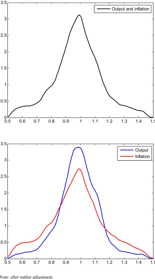
This subsection presents descriptive statistics of relative RMSEs obtained from factor forecasts associated with the total sample (after outliers were removed) and, separately for output and inflation, the different countries/country groups and benchmark models. We are particularly interested in whether factor models are, on average, better or worse than certain benchmark models. We test whether means and medians of relative RMSEs differ significantly from 1 using a t-test and a Wilcoxon sign rank test, respectively. Empirical distributions for the entire sample and for output and inflation separately are shown in Figure 1. Descriptive statistics are provided in Table 2.

The means and the medians for the entire sample and for inflation are roughly at 0.98 and those for output just under 0.99. Although these numbers are only slightly below 1, the tests indicate that, on average, factors models perform significantly better than the respective benchmark models in predicting output and inflation. However, this is associated with more mass in the tails of the empirical distribution of inflation compared to output, as is apparent from the lower panel of Figure 1.

When looking separately at relative RMSEs of different benchmark models, it turns out that factor models perform worse relative to alternative models which are able to exploit large datasets. By contrast, factor models generally outperform small-scale models, with a few exceptions: factor models do worse than ARIMA models and do not significantly differ from VAR models, when predicting inflation. Factor models show the greatest improvements over random walks. It is also notable that single-equation models with indicators perform relatively badly, for instance compared to more simple ARIMA models.

Descriptive statistics for individual countries/country groups clearly indicate that factor models do better than other models on average for the US but worse for the group of other countries (OTHER). This holds for both output and inflation. Results for the UK are not the same for output and inflation; the relative RMSE does not differ significantly from 1 for output but exceeds 1 for inflation. Also interestingly, factor forecasts of euro-area output are outperformed, although not significantly, on average by other models’ forecasts, but factor forecasts of euro-area inflation are clearly superior to other models’ forecasts and the relative RMSE associated to euro-area inflation is even lower than the relative RMSE associated to US inflation. Our findings therefore support the claim of Banerjee et al. (2005) that factor models are better at predicting nominal variables in the euro area compared to the US and real variables in the US compared to the euro area.

The descriptive analysis masks the fact that the various meta-independent variables may interfere with one another. To disentangle the effects, a regression approach is adopted in the next subsection.

4.2. Meta-regression

4.2.1. Baseline meta-regression

We establish the meta-regression equation

j j

j μ φ η

ψ = + 'M + , (8)

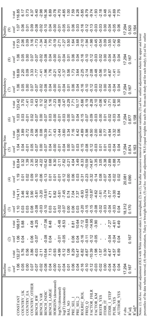
where M_j is the vector of explanatory (meta-independent) variables associated with observation j, _φ is the corresponding vector of coefficients and _μ refers to the overall constant. M_j comprises the continuous variables N, T and HORIZON (as deviations from their arithmetic means) as well as a set of dummy variables into which the discrete variables were transformed. Consider, for example, the variable FACTOR. The dummy variables for the cases FHLR and KM take values of 1 if F_t was estimated with the FHLR and the KM technique, respectively, and 0 otherwise. To avoid perfect collinearity, the SW case is left out. Negative/positive signs of the coefficients of the included dummies indicate lower/higher relative RMSEs, i.e. a better/worse relative factor forecast performance, compared to the cases which were left out. The impacts of the cases which are left out are summarized in the common intercept, which, hence, can be interpreted as the average relative RMSE conditional on the characteristics given by the cases which were left out and on the means of the continuous variables.15 We estimate equation (8) separately for output and inflation, which is

15 _{The constant and the variables’ coefficients can then be used to compute the means of relative RMSEs} conditional on any characteristics, the reader might be interested in.