Posterior population expansion for solving inverse problems
C. J€aggli1 , J. Straubhaar1, and P. Renard11
Centre for Hydrogeology and Geothermics, University of Neuch^atel, Neuch^atel, Switzerland
Abstract
Solving inverse problems in a complex, geologically realistic, and discrete model space and from a sparse set of observations is a very challenging task. Extensive exploration by Markov chain Monte Carlo (McMC) methods often results in considerable computational efforts. Most optimization methods, on the other hand, are limited to linear (continuous) model spaces and the minimization of an objective function, what often proves to be insufficient. To overcome these problems, we propose a new ensemble-based exploration scheme for geostatistical prior models generated by a multiple-point statistics (MPS) tool. The principle of our method is to expand an existing set of models by using posterior facies information for conditioning new MPS realizations. The algorithm is independent of the physical parametrization. It is tested on a simple synthetic inverse problem. When compared to two existing McMC methods (iterative spatial resampling (ISR) and Interrupted Markov chain Monte Carlo (IMcMC)), the required number of forward model runs was divided by a factor of 8–12.1. Introduction
Since the early days of groundwater modeling, inverse methods play a key role in hydrogeology [de Marsily
et al., 2000;Zhou et al., 2014]. They allow inferring the spatial distribution of aquifer parameters (e.g., hydraulic conductivities) from indirect measurements (e.g., piezometric records or the concentration of natural tracers in groundwater). Furthermore, they can also be used to constrain recharge rates or boundary conditions. Inverse modeling is therefore a fundamental step in most quantitative studies since the identification of the parame-ters is a prerequisite for any site-specific model. However, despite its importance and despite more than 50 years of research on this topic, solving the inverse problem still remains one of the hardest challenge. Ground-water flow and transport are often controlled by physical structures that present a high degree of heterogenei-ty. In particular, the underground may contain discrete structures with sharp contrasts of hydraulic properties, such as channels, faults, karst conduits, or lenses. In this case, it can be essential to identify their location very
precisely [Gomez-Hernandez and Wen, 1998;Feyen and Caers, 2006;Linde et al., 2015]. On the other hand, when
inverse methods are specifically designed to consider such geologically realistic and highly complex features, their computational effort often becomes extremely demanding. This problem and the inherited limitations are
not specific to the field of hydrogeology, but are present in most geophysical applications [Linde et al., 2015].
The aim of this paper is to present a new method named PoPEx to overcome a part of those difficulties. But before entering into the description of this method, let us introduce first the general context. The modeling of any geophysical system often requires a complete mathematical description and full parametrization. Solving those equations is referred to solving the forward problem. The solution exists and is unique if the boundary conditions and initial conditions are known. However, in hydrogeology and geophysics, most often the parameters are only known partially and an exhaustive knowledge of their values is lacking. Inverse problems start from a sparse set of observations of the state variables and aim to find the underly-ing set of physical parameter values. Neither existence nor uniqueness of a solution is guaranteed and
therefore, inverse problems are ill posed. The general theory presented byMosegaard and Tarantola[2002]
andTarantola[2005] characterizes the solution of an inverse problem as a conjunction of states of informa-tion. More precisely, the solution is defined as a measure function over a given model space. If this posterior measure function describes a probability distribution, their formulation reduces to the commonly used Bayesianapproach [e.g.,Tarantola, 2005, section 1.5;Box and Tiao, 1973]. In this paper, we only consider problems where both approaches are equivalent. In general, it is very hard or even impossible to find an analytical expression for the solution of an inverse problem.
Key Points:
The paper introduces PoPEx, a new ensemble-based Bayesian inversion method
PoPEx is designed to identify discrete-type models (geological facies)
Numerical tests show that PoPEx is around 10 times more efficient than iterative spatial resampling
Correspondence to:
C. J€aggli,
A possibility for characterizing the posterior probability distribution is to perform an extensive exploration of the model space. One family of pseudorandom exploration schemes is formed by the Markov chain Mon-te Carlo (McMC) methods. The mathematical theory for McMC methods is widely developed and it can be
shown that they are asymptotically ergodic [Robert and Casella, 2004;Bena€ım and Karoui, 2005;Winkler,
2012]. Although they are extensively investigated [Oliver et al., 1997;Fu and Gomez-Hern andez , 2008;Hansen
et al., 2008;Tonkin and Doherty, 2009;Mariethoz et al., 2010a;Hansen et al., 2012;Valakas and Modis, 2016], it is very challenging to design efficient McMC schemes. In short, they are general but their applicability is often drastically restricted by the computational costs. Among the alternative families for solving inverse problems, a very prominent one uses gradient-based optimization of an objective function that may be for-mulated within a Maximum Likelihood (ML) framework. This family of approaches is often used for
address-ing groundwater [Doherty, 2003; Alcolea et al., 2006;Zhou et al., 2011;Li et al., 2012;Xu et al., 2013] or
petroleum engineering problems [Gu and Oliver, 2007;Chen and Oliver, 2013;Melnikova et al., 2015]. These
methods are very efficient to generate models that match observed data [Chen and Zhang, 2006;Zhou
et al., 2011;Xu et al., 2013]. Unfortunately, they require a linear (continuous) model space. Furthermore, the
solution strongly depends on the model parametrization [Mosegaard and Tarantola, 2002;Tarantola, 2005].
This becomes most important whenever a system under study is described by a Jeffrey parametrization. Jef-frey’s parameters are strictly positive physical quantities, as, for example, permeability, speed, and frequen-cy. They are equivalent to their inverses, i.e., resistivity, slowness, and period. It is important that the choice of a specific parametrization for a given inverse problem (e.g., permeability or resistivity, speed or slowness, and frequency or period) must not affect the solution. For a detailed discussion of Jeffrey’s parameters see Mosegaard and Tarantola[2002].
In this paper, we propose a new ensemble-based method, named posterior population expansion (PoPEx) that explores a geologically realistic discrete model space and accounts for an efficient and accurate solu-tion of inverse problems. The discrete random fields are obtained by a multiple-point statistics (MPS)
tech-nique. In general, MPS stands for a pixel-based [Strebelle, 2002;Mariethoz et al., 2010b;Straubhaar et al.,
2011] or pattern-based [Zhang et al., 2006;Arpat and Caers, 2007;Honarkhah and Caers, 2010;Hezarkhani
and Sahimi, 2012;Mahmud et al., 2014] modeling of complex spatial structures derived from a training image (TI). It allows to generate geological patterns that honor imposed data information. The main idea of PoPEx is to expand iteratively an existing set of geological models by using randomly sampled posterior pattern information. In each iteration, the ensemble of models is used to learn, in a statistical sense, the rela-tion between model parameters and state variables. From this point of view, it is inspired by the ensemble
Kalman filter (EnKF) [Burgers et al., 1998;Evensen, 2003, 2006;Chen and Zhang, 2006] but the method neither
computes covariances nor any derivatives of some operator. Both computations can be problematic when
working with discrete model parameters [Linde et al., 2015]. PoPEx is independent of any parametrization
and applicable with any conditional geostatistical simulation tool. It is tested in this paper on a synthetic groundwater flow problem that allows the comparison with a proper reference solution. Comparing the
performance to the one of the McMC schemes presented inMariethoz et al. [2010a], we show that our
algo-rithm provides a slightly better representation of the posterior information while reducing the number of forward model runs by a factor of 8–12. As a counterpart, the property of ergodicity is lost, which means that some region of the model space may not be sampled. Additional tests show that this becomes most important whenever the real spatial structures are poorly captured by the TI.
The paper is organized as follows. Section 2 recalls the formulation of an inverse problem and presents the methodology of our algorithm. An illustrative example is presented in section 3. It aims to highlight the workflow and to show the evolution of the posterior ensemble for the PoPEx algorithm. Then, we empirical-ly anaempirical-lyze the impact of the input parameters and compare the performance of the method with two exist-ing McMC schemes. Section 4 finally discusses the advantages and limitations of the methodology and provides some conclusions.
2. Methodology
In this section, we present the new ensemble-based method, that explores a complex geological model space and accounts for an efficient and accurate characterization of a given posterior density function. Let
us start with some definitions of the terminologies used in this work (section 2.1), before we explain the general concepts (section 2.2) and the details of the new algorithm (section 2.3).
2.1. Inverse Problem Formulation
Solving an inverse problem usually aims to infer information from a given set of observationsd5fd1;. . .;
dmgcalleddata. Usually, these data represent measurements of state variables such as hydraulic heads,
pro-duction data, contaminant concentration, and may include some measurement errors. Mosegaard and
Tarantola[2002] andTarantola[2005] formulate the inverse problem as the characterization of the posterior probability distribution
rMðmÞ5cqMðmÞLðmÞ; (1)
where
cis a normalization constant;
qMðÞdenotes the prior probability distribution;
LðÞis the likelihood function.
In this context, the modelm5fm1;. . .;mngis a finite set of parameters that fully describes the physical
sys-tem under study. Usually the choice of a finite parametrization requires a ‘‘simplification of reality.’’ Such parameters can cover boundary conditions, hydraulic conductivity (or resistivity) fields, specific storage,
recharge time series, etc. Each modelmis a point in a measurable model spaceM. The conceptual choice
of the parametersmicorresponds to the definition of a parametrization ofM. It is clear that this
parametri-zation (i.e., the coordinate system) is not necessarily unique. By definition, the prior probability distribution
qMin equation (1) describes any available information on the model parameters, that is independent of the
observationsd. The likelihood function, on the other hand, describes the correlations between model
parameters and data. It is understood as an indicator of how good a model explains the data and usually involves physical theories that allow to predict the outcome of physical experiments. We assume that the
observable set of data corresponding to a modelmcan be predicted through the so called forward
opera-tord5gðmÞ5fg1ðmÞ;. . .;gmðmÞg. It is possible that the data setd5fd1;. . .;dmgincludes direct
measure-ments of some model parameters inm5fm1;. . .;mng. Although, the proposed method in this paper does
not include this kind of data, it is straightforward to extend it to cases where such observations are avail-able. The remaining components can be predicted by solving a set of partial differential equations
(describ-ing for example groundwater flow) that is fully defined through the model parameters inm. Therefore, the
componentsgiusually include numerical schemes for the solution of differential problems. These numerical
approximations together with the finite parametrization of the system can be a critical source of error. Moreover, due to imperfect measuring devices, the data set itself suffers from uncertainties. It is important
that the likelihood functionLin equation (1) encloses both modeling uncertainties and observational
uncer-tainties. Since the PoPEx algorithm is presented for the first time, we consider a case where the modeling uncertainties are negligible and assume the space of observable data to be linear such that the likelihood
function becomes [Tarantola, 2005]:
LðmÞ5qDðgðmÞÞ: (2)
The probability distributionqD describes any uncertainties and error sources resulting from the act of
observingd5fd1;. . .;dmg. 2.2. General Concepts
This section provides an overview of the general concepts and assumptions used for defining our algorithm.
We assume in this paper that the modelmdescribes spatial petrophysical properties and can be modeled
by a pixel-based MPS algorithm. However, the proposed algorithm is not restricted to MPS and can be applied with many other types of geostatistical models. Pixel-based algorithms require a spatial division of
the computational domain into a finite number ofn2Nhomogeneous grid elements (pixels) within which
the petrophysical properties are constant. Each pixelj2 f1;. . .;ngwill be referred to by its center position
xj. A modelm5fm1;. . .;mngis a set ofnparameters wheremjdenotes a constant petrophysical property
associated to the elementxj. The set of all pixels is called the simulation grid. The MPS algorithm allows to
image. It is possible to condition MPS realizations at a given set of positionsfxi1;. . .;xiNgto a set of values fz1;. . .;zNgsuch thatZðxijÞ5zjfor allj51;. . .;N. In the literature, the collectionHD5fðxi1;z1Þ;. . .;ðxiN;zNÞg
is commonly called hard conditioning data.
In this work, we assume that the random variableZis discrete, i.e., the set of possible values forZðxjÞis
con-tained in a finite subset of real valuesF5ff1;. . .;fsg. The valuesfkfork51;. . .;sare called facies values or
simply facies. Realizations of the random variableZare linked to the model parameters such that there is a bijection between the model spaceMand the set of all possible MPS realizations. Forj51;. . .;n, the mod-el parameter mj denotes then the petrophysical property that corresponds to the facies value ofZatxj.
Figure 1 shows the training image ofStrebelle[2002] defined on a grid of 2503250 pixels and two possible MPS realizations for a grid of 1003100 pixels. The facies values are represented by two different colors (blue forf1and red forf2) and can be associated to two different values of some petrophysical properties
(e.g., permeability, specific storage, and porosity). If, for example, we want to use this two-facies setup for modeling spatial groundwater permeability maps, we choose a set of two different permeability values
fK1;K2gand define the one-to-one correspondence
Ki$fi; i51;2:
Thanks to this bijection between model parameters and facies values, the petrophysical modelmis unique-ly defined by the facies map of an MPS realization and vice versa. It is for this reason that in the following, we will interchangeably use the terminologies ‘‘realization’’ and ‘‘model’’ by referring to their spatial map defined in the simulation grid. The concept of a pixel-based indicator function for each facies value will be important. Thus, for any modelm, we define the characteristic indicator function1fi at each pixelxj such
that 1fiðm;xjÞ5 1 ifmj$fi 0 otherwise: ( (3)
Henceforth, the explicit notation of the pixel positionxjwill be omitted. Therefore, the indicator functions
in equation (3) and any inherited quantity can be interpreted as maps that are defined on the simulation grid and are constant within each pixel.
The main idea of the posterior population expansion (PoPEx) algorithm is to expand an existing set of mod-elsMk5fm
1;. . .;mkgby using facies information that is weighted by the posterior measure function in
equation (1). For each modelmjinMk, we compute the corresponding posterior informationrMðmjÞand
form the setR~k5f~rMðm1Þ;. . .;~rMðmkÞgwhere
~ rMðmjÞ5 r MðmjÞ Xk r51rMðmrÞ ; j51;. . .;k
are the normalized values of the posterior information. For a facies valuefi, we define its posterior
probabili-ty mappk i by pk i5 Xk j51 1fiðmjÞ~rMðmjÞ: (4)
Similarly, for each facies typefi, we suppose to know prior probability mapsqi. Usually it is possible to
approximate the prior probability maps from a sufficiently large number of unconditioned (i.e., without any hard-conditioning data) and independent MPS realizations. The key is then to compare the two probability distributionsPk5fpk
1;. . .;pksgandQ5fq1;. . .;qsgby means of the Kullback-Leibler divergence (KLD) [ Kull-back and Leibler, 1951], denoted byDðPkjjQÞand reading
DðPkjjQÞ5X s i51 pk i log pk i qi : (5) Remember thatpk
i,qi, and thereforeDðPkjjQÞare maps defined on each pixel in the simulation grid.
Rough-ly speaking, the Kullback-Leibler divergence ofPkfromQprovides a measure of how different or
‘‘surpris-ing’’ the posterior facies probabilities inPkare with respect to the prior probabilities inQ. The idea is then to
deduce a set ofNChard conditioning data from which one new MPS realization will be generated. First, the
conditioning locationsxij are sampled from a probability density function that is proportional to the KLD
mapDðPkjjQÞ. Then, for each location, we sample a conditioning valuez
jfrom the restricted posterior
prob-abilities pk
iðxijÞ. After the generation of a new realization conditioned to the collection
HD5fðxi1;z1Þ;. . .;ðxiN;zNÞg, it is added to the existing set of modelsM
k
and the posterior measurerMis
computed. Then, the entire procedure is restarted. An illustrative example of the workflow is presented in section 3.4 in Figure 3.
2.3. Posterior Population Expansion (PoPEx)
The approach described above assumes to know an existing set of modelsfm1;. . .;mkg. Therefore, at the
very beginning, we have to generate at least one initial realization. But it is clear that it can be
advanta-geous to start from a larger number ofNI>1 unconditioned and independent initial models. We will see in
section 3 that not onlyNIbut also the number of conditioning dataNCplay an important role. Both
parame-ters are predefined by the user and stay unchanged during the whole procedure. Let us now define the PoPEx algorithm:
1: Input:NI2Nnf0g and NC2N
2: Initialization: Generate NI unconditioned models
3: Set:k5NI and Mk5fm1;. . .;mkg
4: Compute: R~k,Pk andDðPkjjQÞ 5:whilestopping condition 5= false do
6: ChooseNC conditioning data pairs fromPk and DðPkjjQÞ
7: Generate one conditioned realization mk11
8: SetMk115Mk[ fmk11g
9: Compute R~k11;Pk11 and DðPk11jjQÞ
10: Update stopping condition
11: k5k11
12:end while
Note thatR~kis the normalized posterior information inMkand therefore, this algorithm is independent of
the normalization constantcin equation (1). For this reason, the posterior informationrMðmÞcan be
com-puted by simply settingc51. Furthermore, the Kullback-Leibler divergence in equation (5) is well defined
forqi>0 for alli51;. . .;s. If there isi2 f1;. . .;sgand a pixelxjsuch thatqiðxjÞ50, then the prior measure
corresponding terms in equation (5) are put to zero. For an illustration of the workflow applied to the syn-thetic problem introduced in the section 3, consult Figure 3.
Let us look in more detail at the most important steps. The two main inputs of this algorithm are the
number of unconditioned initial modelsNIand the number of conditioning dataNC. [2] Initially,NI
uncon-ditioned and independent models are generated. Note that at this point we suppose to know the prior
facies probability maps inQ5fq1;. . .;qsg. If such maps are unavailable andNIis large enough, they may
be approximated from the initial set of unconditioned realizations. Then, with the posterior information of
each model, we compute the probability map Pkand update the corresponding Kullback-Leibler
diver-genceDðPkjjQÞ(cf. equations (4) and (5)). [6] The central point of the PoPEx algorithm is the way of fixing
a hard-conditioning data setHD5f ðxi1;z1Þ;. . .;ðxiNC;zNCÞ g that guides the generation of a new model.
For this purpose, we choose the locations xij randomly from a probability distribution proportional to
DðPkjjQÞ. This preferentially selects conditioning locations where the posterior probabilityPkhas a high
information content with respect to the prior probabilityQ. The valueszjthat are imposed atxij are then
picked according to the probability values ofPkatxij. Large values of the KLD mapDðP
kjjQÞshow
loca-tions where the approximated posterior facies distribution diverges a lot from its prior counterpart. By imposing facies values within such pixels, we expect to increase the probability of generating models
with high posterior measure. In steps [8] and [9], the model spaceMk is expanded to Mk11 before
the posterior information setR~k11, the facies probability mapPk11and the Kullback-Leibler divergence
DðPk11jjQÞare computed. [10] There are different possible stopping criteria, each of which has its
justifi-cations and can be chosen according to the needs. As the forward operator, and therefore the computa-tion of the posterior informacomputa-tion, can be very expensive in terms of computacomputa-tional cost, we may want to restrict the runtime of the algorithm. Thus, an obvious stopping condition is to set a maximum size of the final population. Sometimes, one may want to use an acceptance/rejection criterion based on the
value of the likelihood functionLðmÞto generate a fixed number of accepted models. A third criterion
is the convergence of the posterior facies probability distribution map Pk. In this case, at every step
k>NI, the distributionPkis compared toPk2j, for aj1, and the algorithm is stopped as soon as the
difference is small enough.
A very important feature of this algorithm is its independence of any physical parametrization. The only ran-dom variables involved are characteristic indicator functions, and therefore, the algorithm is independent of the facies values and all the physical parameters they are associated with. As every new model is depending on all the previous ones, however, there is a risk of exploring only a restricted subregion of the model space. But, we can increase the research area in the model space by increasing the number of unconditioned initial
realizations and/or lower the number of conditioning data. An empirical analysis of the choice ofNIandNC
is provided in the section 3.4.
3. Synthetic Case Study
As this paper introduces the PoPEx algorithm for the first time, it is a prerequisite to test it under simple and well-defined conditions where a reference solutions can be computed. This is why we borrowed the
two-dimensional groundwater flow problem fromMariethoz et al. [2010a]. This small problem is briefly explained
in the following section. 3.1. Problem Setting
The mathematical model of a two-dimensional (stationary) groundwater flow problem is described by the Poisson equation:
2divðkrhÞ5f: (6)
The solution h:D!R is usually defined in a bounded, open, and Lipschitz domain DR2, and
describes the hydraulic head level of the groundwater. Together with reasonable boundary conditions,
the problem (6) is well posed. As inMariethoz et al. [2010a], the spatial models were defined by
channel-ized structures simulated from the training image in Figure 1a. The two facies types represent uniform
transmissivity (k) values of 1022(m2/s) (channel) and 1024(m2/s) (matrix), respectively. For modeling the
spatial structures, we used the DeeSse implementation [Straubhaar, 2011] of the MPS direct sampling (DS)
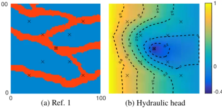
containing 100 by 100 pixels and rep-resenting a 100 m by 100 m computa-tional domain. The model space was set to be the space of all possible models generated by the DS method. On the upper and lower boundaries, no-flow boundary conditions applied, while fixed head values of 1 m (left) and 0 m (right) were imposed on the lateral boundary parts. One realization with an arbitrary seed has been gener-ated and considered to be the refer-ence domain (cf. Figure 2a). A pumping well extracting 3 L/s was placed in the center of the domain (square), while at nine locations (crosses), we extracted the hydraulic head values of the numerical reference solution (cf. Figure 2b); these measurements of the groundwater level were the only data constraints used for conditioning the inverse problem. We set the prior distributionqMin equation (1) to be uniform. As in this case, the prior information is constant for any modelm, the PoPEx algorithm only depends on the value of the likelihood functionL. Using again the fact that the posterior information in equation (1) can be multiplied by any positive constant without chang-ing the behavior of the algorithm, the likelihood function can be rewritten such that
LðmÞ5exp 2RMSEðmÞ 2
2r2
!
; (7)
where RMSEðmÞdenotes the root-mean-square error between the predictions and the reference values. The standard deviation is set tor50:05 m, what reasonably matches measurement errors met in practice.
3.2.IllustrationofthePoPExAlgorithm
Before starting the analysis of the algorithm let us use the previously defined problem for illustrating the key steps of our algorithm. We fix the input parameters toNI5200 andNC515. Figure 3 shows the
evolu-tion of the different maps. It is separated into multiple parts. The two figures in the top row are the fixed pri-or probabilities fpri-or each facies type. Fpri-or this synthetic example, the mapsq1andq2take constant values of
0.72 and 0.28, respectively. Then, the first two columns of the matrix on the bottom illustrate the posterior probability mapsp1andp2at the iterations k5200, 500, and 2000. The third column is the normalized
Kullback-Leibler divergence D~ðPkjjQÞ. During each iteration, we use the probability density D~ðPkjjQÞ for
samplingNChard conditioning locations. Red dots are used to indicate the locations that have been picked
at iterationk5200, 500, and 2000, respectively. After having fixed the conditioning locationsfxi1;. . .;xiNCg,
conditioning facies values zj are sampled from the localized facies probability maps PkðxijÞ5fpk1ðxijÞ; pk
2ðxijÞg, forj51;. . .;NC. The last column shows the new modelmk11that was generated from the
hard-conditioning data setfðxi1;z1Þ;. . .;xiNC;zNCg(indicated by the black dots). Note that, due to the definition
of the prior probability maps, high probability values in the mapp2contain more information in the sense
that they are more surprising with respect to the prior probability distribution than high probability values inp1. As mentioned earlier,D~ðPkjjQÞcan be interpreted as a measure of information contained inPkwith
respect toQ.
3.3.DescriptionoftheTestProcedures
The synthetic test problem described above has been chosen because it allows to compute an empirical ref-erence set of 300,000 models that represents a good approximation of the entire model space. From this large set of models, any quantity of interest can be computed and will be considered as the exact solution. If, for instance, we are interested in the true posterior expectation of a quantity represented by a function
fðmÞ, we use this set of models and compute the reference solution such that
X
300;000
i51
fðmiÞ~rMðmiÞ: (8)
Again,~rMdenotesthenormalizedposteriorinformation.ForanevaluationofthePoPExalgorithm,we
formu-latedfourdifferenttestprocedures.Beforepresentingsomeresultsletusexplaineachexperimentindetail.
3.3.1.TestI:InfluenceoftheInputParametersNIandNC
Thegoalofthisfirsttestistoempiricallyanalyzetheinfluenceofthenumberofunconstrainedinitial mod-elsNIandthenumberofconditioningdataNC.Wewereinterestedinthediversityofthegeneratedmodels
andthereforeonhowwellthealgorithmisabletoexplorethemodelspace.Equation(8)togetherwith equation(3)areusedforcomputingthereferenceposteriorprobabilitymapsPref5fp
1 ref;p
2
refg.Then,for
dif-ferentnumbersNIandNC,werunthePoPExalgorithmuntil4000conditionedrealizationshavebeen
gener-ated.Asameasureoftheexplorationcapability,wecomputedthemeanvalueoftheKLDmapDðPkjjPrefÞ.
Inotherwords,ifthismeanvalueislow,theposteriorfaciesprobabilitiesinPkareclosetothereference onesandtherefore,thealgorithmreasonablysampledthemost‘‘importantsubregions’’ofthemodelspace. Inthiscontext,‘‘important’’standsforareaswheretheposteriormeasurerMissufficientlylarge.Wewere
mostlyinterestedintheregionsexploredbytheconditionedrealizations(i.e.,fork>NI),andtherefore,Pk
wascomputedwithouttheNIinitialmodels.
The next two tests are dedicated to compare the PoPEx algorithm with two existing Markov Chain Monte Carlo (McMC) schemes.
Figure 3.Workflow of the PoPEx algorithm applied to a synthetic two-facies problem. The prior and posterior facies probability maps together with the resulting Kullback-Leibler divergence mapD~ðPk11jjQÞare shown for the iterationsk5200, 500, and 2000. The last col-umn to the right shows the new realization that has been conditioned at the locations indicated by dots.
3.3.2. Test II: Comparing the Exploration Capabilities
There are different McMC techniques available for solving inverse problems in a geostatistical prior model
space. The ones presented inMariethoz et al. [2010a] were entitled iterative spatial resampling (ISR) and
interrupted Markov chain Monte Carlo (IMcMC). Central for both algorithms is the definition of a likelihood
functionLas in equation (7). The ISR method uses an MPS technique for the generation of a chain of models
ðm1;. . .;mn;. . .Þ. At every instancen>0, it extracts facies values frommnand uses them as hard
condition-ing data for the generation of a candidate modelm. This model is then accepted with a probability of
minf1;LðmÞ=LðmnÞg. Conversely, the IMcMC method accepts a new model wheneverLðmÞ LðmnÞand
interrupts and restarts the chain according to a suitable stopping condition. For both McMC methods,
Mar-iethoz et al. [2010a] fixed a number of 100 conditioning points. As suggested, the burn in period in the ISR method was set to be the first 200 accepted realizations, while the IMcMC chain was interrupted whenever
RMSEðmiÞ 0:07 m: (9)
This corresponds to the 95% confidence interval of the data distribution defined by nine independent observations with Gaussian errors.
For comparing the exploring skills, we considered the first 4000 realizations generated by ISR after the burn in time. There is no particular initial stage in the IMcMC method, so we took all the realizations into account.
As in the first test, fork51;. . .;4000 and for each algorithm, we form the weighted facies probability map
Pkand compare it toPrefby the KLD mapDðPkjjPrefÞ. Again, a low mean value of the latter is interpreted as
a good exploration of the important regions in the model space. 3.3.3. Test III: Comparing the Efficiency and Data Predictions
Depending on the computational cost of a prediction, it can be very expensive to compute the correspond-ing random variable for a large number of models. Therefore, we often evaluate it only on a representative subset of models. Using Markov chain Monte Carlo methods, one usually fixes the size of a characteristic (representative) set and stops the algorithm as soon as enough models have been accepted. For analyzing the efficiencies of the methods, we generated a representative set of 200 models satisfying the condition in equation (9) and compared the total numbers of forward simulations needed.
Groundwater production problems often involve the prediction of the capture zone within a given time
T>0. Therefore, we defined the random variableZT5ZTðm;xjÞto be a characteristic indicator function
such thatZTðm;xjÞ51, if a water particle starting atxjreached the pumping well in a time no longer thanT,
andZTðm;xjÞ50 otherwise. The posterior pumping area was defined as
AT5
X m
ZTðmÞr~MðmÞ:
ForT520 h and based on 300,000 unconditioned realizations, we computedAref
T and compared it to the
posterior pumping areas computed for the representative sets of 200 models satisfying equation (9). The last test aims to discover the applicability and some limitations of the method.
3.3.4. Test IV: PoPEx Solutions for Different Reference Domains
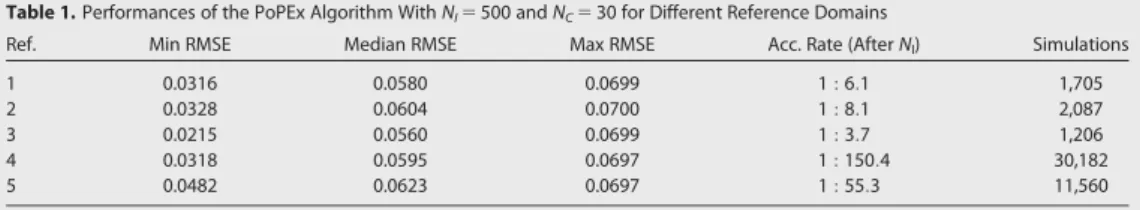
The performance of an inverse method can depend very much on the unknown geology. Therefore, it is important to run the algorithm with data sets (observations) coming from different reference domains. To this end, we generated four additional reference maps and kept the differential problem and the observa-tion locaobserva-tions unchanged. The performances are mainly compared by the number of forward simulaobserva-tions needed in order to generate a representative set of 200 models satisfying equation (9).
3.4. Results
This section presents the results obtained from the four tests described above. Note that the results have been obtained by running each experiment 5 times, starting from five different initial sets. We then show their average performances.
3.4.1. Test I
When we fix the number of conditioning dataNCand vary the number of unconstrained initial models
NI2 f100;200;500;1000g, we clearly observe a better examination of the model space for higher values of
NI(cf. Figures 4a and 4b). Comparing the two figures we conclude also that in general we had better
4cand4d,wherethenumberofunconditionedinitialmodelsNIwasfixedandwechangedthenumberof
conditioningdataNC 2 f15;30;45;60g.However,ahighernumberofconditioningpointsresultedina
fasterconvergenceinthebeginningandtheposteriorprobabilitymapsbecamestationaryafterasmaller
numberofiterations.Wefinallysuggestthatforafastconvergenceweshouldnotchooselessthan30
con-ditioningpoints,butinordertoreasonablyexaminethemodelspace,weshouldstartwithatleast200
unconditionedinitialrealizations.
3.4.2.TestII
Accordingtotheprevioustest,areasonablechoiceforthePoPExalgorithmwasNC530andNI2 f200;
500g.ThePoPExandtheISRmethodsshowedverysimilarbehaviorinapproximatingPref,whiletheIMcMC
tookslightlymoretimetoconvergetoastationarylevel(Figure5).Althoughalltheinterruptedchainsinthe
IMcMCmethodareindependentofeachother,thismethodwasnotabletoreachtheapproxi-mationlevel
ofthePoPExalgorithm.Whenwecomputedthereferenceposteriorprobabilityofthechannelfacies(p2ref)
andcomparedittothemapspk
2obtainedafter4000simulations,weobservedsignificantdiffer-ences
(Figure6).Thesharpcontrastsofthereferencemap(Figure6a)werealmostentirelymissinginthe
IMcMCmap(Figure6d).TheISRpicture(Figure6c)
mainlyshowsthreeparalleldownwardstructures.The
lessercontrastedsmallbifurcationsintherightpartof
thefigurecouldonlybediscoveredbythePoPEx
algo-rithm(NI5500,cf.Figure6b).Therefore,althoughthe
differencesinFigure5seemedtobesmall,itwaseasyto
seethatthePoPExalgorithmclearlygeneratedthebest
approximationofthereferencefaciesprobabilitymap.
3.4.3.TestIII
SettingagainNC530, weobservethatinaveragethe
twoPoPExalgorithmsonlyneeded1705(NI5500)resp.
1935 (NI5200) simulations, while the McMC methods
required 15,698 (ISR) and 21,052 (IMcMC) forward
Figure 4.Approximation of the posterior facies probability map for (top) variableNCand fixedNI, resp. and (bottom) fixedNIand variable
NC.
Figure 5.KLD convergence during 4000 realizations for two different settings of the PoPEx algorithm compared to ISR and IMcMC.
simulations, respectively (cf. Figure 7). The generation of unconditioned realizations can be interpreted as a simple rejection sampler and required 42,136 simulations. As suggested byMariethoz et al. [2010a] in the Markov chains, we only considered realizations that are at a distance of at least 12 accepted models. The results in this section showed that for generating a slightly better approximation of the posterior facies probabilities (cf. Figures 5 and 6), the PoPEx algorithms were roughly 8–9 (resp. 11–12) times more efficient than ISR (resp. IMcMC) and more than 20 times faster than rejection sampling (cf. Figure 7). The overall acceptance rates of the PoPEx algorithms were 1:8:5 (NI5500) resp. 1:9:7 (NI5200), while they reached
1:6:1 and 1:8:7, when considering only the conditioned realizations.
Asallofthethreealgorithms(PoPEx,ISR,andIMcMC)generatedcharacteristicsetswithsufficientvariability ofthemodels,theyallproducedaccuratepredictionsofthereferenceregionsandthetruecapturezone (cf.Figure8).Nevertheless,westillobservesomedifferences.ThepredictionsofthePoPExandtheISR algo-rithmmostdifferinthe5%regionbutbothweresufficientlyclosetothereferencemap.The5%and25% regionsoftheIMcMCmethodwereslightlytoobroad.Recallingtheresultsobtainedintheprevioustest, thiswasnotsurprising,asIMcMCshowedtheworstapproximationoftheposteriorfaciesprobabilities.
3.4.4.TestIV
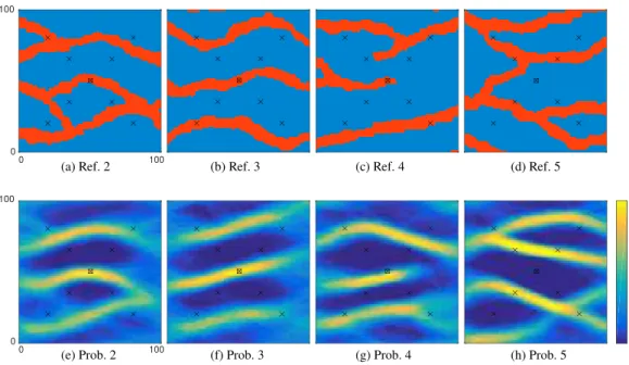
The structures in thefirst two additional domains (Ref. 2 andRef.3 in Figures9a and 9b) correspond well to theones inthe training image (cf. Figure 1a). The third(Ref. 4 inFigure 9c) shows two inter-ruptedchannelsnearthepumpingwell. Asthetrainingimagedoesnotcontainanydisconnected chan-nels, it was veryunlikely to generatesuch models by anMPSmethod. Inthe fourthdomain (Ref. 5in Figure 9d), nochannel passthrough thepumping location.From a physical point of view,this means that3Lofwaterareextractedeverysecondfroma low-permeablematerial, whichwouldbeabsurd.As before we use thehydraulic head values extractedfrom the reference solution as data constraintsfor solving theinverse problems.According tothepreviousanalysis, wegeneratedNI5500unconditioned
initialmodels andused NC530conditioningpoints,until200models satisfied(9).Thestructuresinthe
referencedomains1and2(Figures2aand9a)showcomparablegeologicalpatterns.Both are dominat-ed by three interconnectedand bifurcated main channels, linking theleft tothe right boundary part. For solving theinverse problems, comparable numbers of forward simulations (1705, resp. 2087) were needed(cf. Table1).It turnedoutthattheproblemcorrespondingtothethirdreferencedomain(Ref.3 in Figure 9b) was relatively easy to solve. The sepa-rated and mostly parallel channels match the struc-tures of the training image quite well. It follows that, after only 1206 models, the algorithm was able to find 200 satisfying models. Also, the minimum and the median RMSE values are considerably low (cf. Table 1). Both of the posterior channel probability maps pk
2 (Figures 9e and 9f) describe fairly well the
main structures of the corresponding reference domains (Ref. 2 and Ref. 3) but still show sufficient variability in other regions of the computational domain (where the posterior probabilities are close to the prior probabilities).
Figure 6.Posterior probability mapspk
2obtained after 4000 realizations.
Figure 7.Comparison of the efficiencies for generating a set of 200 accepted models.
For revealing some limits of the PoPEx algorithm, we chose the uncommon reference domains Ref. 4 and Ref. 5. The large number of simulations (Table 1) needed for solving the inverse problem resulting from Ref. 4 (Figure 9c) was directly related to its interrupted channel structures. As there are no such patterns con-tained in the training image, it is very unlikely to generate good candidate models. Although the method was able to detect this unusual structure (Figure 9g), the number of total simulations and the acceptance rate were unacceptable (Table 1). This highlighted the importance of a reliable training image that repre-sents well the geological features. On the other hand, extracting 3 L of groundwater per second from a low-permeable region (Figure 9d) is physically not very plausible. The hydraulic head of the reference solution at the pumping well is219.1 m, from what follows that the range of the head values is significantly larger. Working with the same (absolute) acceptance tolerance (equation (9)) leads to accept only small relative errors and therefore explains the slower acceptance rate in Table 1 (Ref. 5) and the smaller variability of the posterior models (Figure 9h). The high values of the corresponding minimum and median RMSE also indi-cate the difficulties to reach the same (absolute) approximation level for a larger range of head values. A stopping criterion based on a minimum number of accepted realizations can require a large number of for-ward simulations and therefore, significantly grows the computational costs for solving an inverse problem. We conclude that the PoPEx algorithm was very efficient and accurate in solving inverse problems with facies-type prior models. However, unreasonable stopping conditions and/or a nonrepresentative training image result in unacceptable high computational costs.
Figure 8.Posterior predictions of the capture zone after 20 h of pumping. The contours are understood as the percentage coverage of a certain region by the 200 representative models.
Figure 9.Reference domains 2–5 and their corresponding posterior channel probability maps of 200 accepted models (using PoPEx with NI5500 andNC530).
4. Discussion and Conclusions
In this paper, a new ensemble-based method, entitled posterior population expansion (PoPEx), is proposed. We show on a simple and synthetic example that it efficiently sampled the most important regions (with respect to the posterior information) of a complex and discrete model space. Comparing our method to two existing McMC schemes, we showed that PoPEx explored the posterior probability distribution more accurately and considerably reduced the computational costs. The small number of input parameters and their intuitive influence on the behavior of the method makes its usage very easy. The entire procedure is independent of any model parametrization. However, we showed also that the quality of the training image and the stopping condition are very important.
A broad range of existing methods for solving inverse problems that are based on the minimization of a misfit function are particularly efficient if three main assumptions are fulfilled: the model space and the data space are linear, their uncertainty is described by a Gaussian probability distribution and they are
con-nected through a linear forward operator [Arulampalam et al., 2002;Mosegaard and Tarantola, 2002;
Taran-tola, 2005]. In the hydrogeological framework, however, usually none of the assumptions are satisfied. In
order to overcome these requirements, nonlinear transformations into Gaussian spaces [Zhou et al., 2011;Li
et al., 2012;Xu et al., 2013;Xu and Gomez-Hernandez, 2015], linear approximations of the forward operator [Chen et al., 2009] and simplified parametrizations from Gaussian subspaces [Doherty, 2003;Alcolea et al.,
2006;Tonkin and Doherty, 2009] have been extensively investigated. Unfortunately, it is not possible in
gen-eral to meet all of the three assumptions. The core of the PoPEx algorithm however, has been designed for cases in which the model space is discrete and well adapted to account for prior geological knowledge which can be expressed via an MPS or any other conditional geostatistical simulation tool. MPS methods were chosen because they have proven to be a very powerful tool for modeling complex and
heteroge-neous geological environments in real applications [Caers et al., 2003;Liu et al., 2004;Okabe and Blunt, 2007;
Ronayne et al., 2008]. Overall, the proposed algorithm is potentially able to solve sophisticated inverse prob-lems. In this work, we only considered spatial uncertainties that represented different rock types. Neverthe-less, it is possible to acknowledge any kind of uncertainties that can be modeled by conditional simulations.
The same complexity of the model space can be covered by McMC methods [Alcolea and Renard, 2010;
Mar-iethoz et al., 2010a;Hansen et al., 2012;Laloy et al., 2016]. The ergodicity of Markov chains ensures an asymp-totic exploration of the true posterior information. In practice, however, the convergence of McMC methods is slow.
The PoPEx algorithm, on the other hand, does not fulfill the property of ergodicity. Assume thatMk5fm1;
. . .;mkgis a sufficiently large subset of the model spaceMsampled from a probability measure function
rM:M !R. An unbiased estimator [Durrett, 2010] of the first moment (with respect torM) of a random
variablef:M !Ris given by ^ l51 k Xk i51 fðmiÞ: (10)
Likewise, ifMkrepresents an uniformly distributed subset ofM, the first moment can be approximated by
the weighted sum [Robert and Casella, 2004]
^
l5X
k
i51
fðmiÞr~MðmiÞ: (11)
In the PoPEx algorithm, the equation (4) used for computing the posterior probability maps are of the form of expression (11) above. The distribution of the PoPEx realizations, however, is clearly not uniform for
Table 1.Performances of the PoPEx Algorithm WithNI5500 andNC530 for Different Reference Domains
Ref. Min RMSE Median RMSE Max RMSE Acc. Rate (AfterNI) Simulations
1 0.0316 0.0580 0.0699 1:6:1 1,705
2 0.0328 0.0604 0.0700 1:8:1 2,087
3 0.0215 0.0560 0.0699 1:3:7 1,206
4 0.0318 0.0595 0.0697 1:150:4 30,182
k>NI. If a large number of conditioned realizations has been generated, we expect that the models inMk
are distributed according to a density that is close (in some sense) to the posterior measurerM. Therefore,
using weighted sums as in equations (4) and (11) overestimates regions of high posterior information (see
e.g., fundamental identity of importance sampling inRobert and Casella[2004]). In the early iterations of the
PoPEx method, the number of conditioned models is small and the slight overestimation helps to accelerate the algorithm. In the long term, however, it results in a reduced variability of the posterior models (cf. Fig-ures 6a and 6b).
Let us briefly comment on our choice of the prior probability measure function. The sequential construction of the spatial models by a DS technique depends on the uniformly distributed random paths that run
through the pixels. IfNdenotes the number of pixels andsthe number of facies types, there areN!different
paths but no more thansNdifferent models. Therefore, for largeN, the map sending a path onto the
corre-sponding model is not injective (asN!>sN). It follows that there are different paths that produce the same
realization. By defining an appropriate distance between the models and the training image, we may observe that models with ‘‘common’’ structures are ‘‘closer’’ than others. We expect that such ‘‘common’’ realizations have a higher probability of occurrence. Thus, the MPS algorithm does not produce different models with uniform probability. A distance between the TI and the models could be used for the definition of a suitable prior distribution. However, defining a reasonable distance for facies-type models is far from being trivial. This is why, for this work, we assumed uniformity of the prior distribution.
Although the presented algorithm showed promising behavior on a synthetic problem, let us remark that a complete analysis should involve a more complex field study (with a number of model parameters on the
order of 1062108. In such cases, modeling uncertainties and nonuniformity of the prior distribution usually
can no longer be neglected. Both are matters that should be further investigated.
References
Alcolea, A., and P. Renard (2010), Blocking Moving Window algorithm: Conditioning multiple-point simulations to hydrogeological data,
Water Resour. Res.,46, W08511, doi:10.1029/2009WR007943.
Alcolea, A., J. Carrera, and A. Medina (2006), Inversion of heterogeneous parabolic-type equations using the pilot points method,Int. J. Numer. Methods Fluids,51(9-10), 963–980.
Arpat, G. B., and J. Caers (2007), Conditional simulation with patterns,Math. Geol.,39(2), 177–203.
Arulampalam, M. S., S. Maskell, N. Gordon, and T. Clapp (2002), A tutorial on particle filters for online nonlinear/non-Gaussian Bayesian tracking,Trans. Signal Processing,50(2), 174–188.
Bena€ım, M., and N. E. Karoui (2005),Promenade Aleatoire: Cha^ınes de Markov et Simulations: Martingales et Strategies, Math. Appl.Ecole Poly-tech., Palaiseau Cedex, France.
Box, G. E., and G. C. Tiao (1973), Bayesian Inference in Statistical Analysis, Behav. Sci. Quant. Methods, Addison-Wesley., Boston, Mass. Burgers, G., P. J. van Leeuwen, and G. Evensen (1998), Analysis scheme in the ensemble Kalman filter,Mon. Weather Rev.,126(6), 1719–1724. Caers, J., S. Strebelle, and K. Payrazyan (2003), Stochastic integration of seismic data and geologic scenarios: A West Africa submarine
chan-nel saga,Leading Edge,22(3), 192–196.
Chen, Y., and D. S. Oliver (2013), Levenberg-Marquardt forms of the iterative ensemble smoother for efficient history matching and uncer-tainty quantification,Comput. Geosci.,17, 689–703.
Chen, Y., and D. Zhang (2006), Data assimilation for transient flow in geologic formations via ensemble Kalman filter,Adv. Water Resour.,
29(8), 1107–1122.
Chen, Y., D. S. Oliver, and D. Zhang (2009), Data assimilation for nonlinear problems by ensemble Kalman filter with reparameterization,
J. Pet. Sci. Eng.,66(1–2), 1–14.
de Marsily, G., J. P. Delhomme, A. Coudrain-Ribstein, and A. M. Lavenue (2000), Four decades of inverse problems in hydrogeology,Geol. Soc. Am. Spec. Pap.,348, 1–17.
Doherty, J. (2003), Ground Water Model calibration using pilot points and regularization,Ground Water,41(2), 170–177. Durrett, R. (2010),Probability: Theory and Examples, Stat. Probab. Math., Cambridge Univ. Press, New York.
Evensen, G. (2003), The ensemble Kalman filter: Theoretical formulation and practical implementation,Ocean Dyn.,53(4), 343–367. Evensen, G. (2006),Data Assimilation: The Ensemble Kalman Filter, Springer-Verlag, New York.
Feyen, L., and J. Caers (2006), Quantifying geological uncertainty for flow and transport modeling in multi-modal heterogeneous forma-tions,Adv. Water Resour.,29(6), 912–929.
Fu, J., and J. Gomez-Hernandez (2008), Preserving spatial structure for inverse stochastic simulation using blocking Markov chain Monte Carlo method,Inverse Problems Sci. Eng.,16(7), 865–884.
Gomez-Hernandez, J. J., and X.-H. Wen (1998), To be or not to be multi-Gaussian? A reflection on stochastic hydrogeology,Adv. Water Resour.,21(1), 47–61.
Gu, Y., and D. S. Oliver (2007), An iterative ensemble Kalman filter for multiphase fluid data assimilation,Comput. Geosci.,12(4), 438–446. Hansen, T. M., K. Mosegaard, and K. S. Cordua (2008), Using geostatistics to describe complex a priori information for inverse problems, in
8th International Geostatistics Congress, pp. 329–338, Gecamin.
Hansen, T. M., K. S. Cordua, and K. Mosegaard (2012), Inverse problems with non-trivial priors: Efficient solution through sequential Gibbs sampling,Comput. Geosci.,16(3), 593–611.
Hezarkhani, P. T. A., and M. Sahimi (2012), Multiple-point geostatistical modeling based on the cross-correlation functions,Comput. Geosci.,
16(3), 779–797.
Acknowledgments
The authors would like to thank Michael Pyrcz, the two anonymous reviewers, and the Editors for their many helpful suggestions. They have greatly helped to improved the presentation of this paper. This work was funded by the Swiss National Science Foundation through the grant 153637. The data and codes used to generate the results of this paper can be obtained from the corresponding author ([email protected]).
Honarkhah, M., and J. Caers (2010), Stochastic simulation of patterns using distance-based pattern modeling,Math. Geosci.,42(5), 487–517. Kullback, S., and R. A. Leibler (1951), On information and sufficiency,Ann. Math. Stat.,22(1), 79–86.
Laloy, E., N. Linde, D. Jacques, and G. Mariethoz (2016), Merging parallel tempering with sequential geostatistical resampling for improved posterior exploration of high-dimensional subsurface categorical fields,Adv. Water Resour.,90, 57–69.
Li, L., H. Zhou, H. J. Hendricks Franssen, and J. J. Gomez-Hernandez (2012), Groundwater flow inverse modeling in non-MultiGaussian media: Performance assessment of the normal-score Ensemble Kalman Filter,Hydrol. Earth Syst. Sci.,16(2), 573–590.
Linde, N., P. Renard, T. Mukerji, and J. Caers (2015), Geological realism in hydrogeological and geophysical inverse modeling: A review,Adv. Water Resour.,86, 86–101.
Liu, Y., A. Harding, W. Abriel, and S. Strebelle (2004), Multiple-point simulation integrating wells, three-dimensional seismic data, and geolo-gy,AAPG Bull.,88(7), 905–921.
Mahmud, K., G. Mariethoz, J. Caers, P. Tahmasebi, and A. Baker (2014), Simulation of Earth textures by conditional image quilting,Water Resour. Res.,50, 3088–3107, doi:10.1002/2013WR015069.
Mariethoz, G., P. Renard, and J. Caers (2010a), Bayesian inverse problem and optimization with iterative spatial resampling,Water Resour. Res.,46, W11530, doi:10.1029/2010WR009274.
Mariethoz, G., P. Renard, and J. Straubhaar (2010b), The direct sampling method to perform multiple-point geostatistical simulations,Water Resour. Res.,46, W11536, doi:10.1029/2008WR007621.
Melnikova, Y., A. Zunino, K. Lange, K. S. Cordua, and K. Mosegaard (2015), History matching through a smooth formulation of multiple-point statistics,Math. Geosci.,47, 397–416.
Mosegaard, K., and A. Tarantola (2002), 16 - Probabilistic approach to inverse problems, inInternational Handbook of Earthquake and Engi-neering Seismology, Part A, International Geophysics, vol. 81, edited by P. C. J. William et al., pp. 237–265, Academic Press, U. K. Okabe, H., and M. J. Blunt (2007), Pore space reconstruction of vuggy carbonates using microtomography and multiple-point statistics,
Water Resour. Res.,43, W12S02, doi:10.1029/2006WR005680.
Oliver, D. S., L. B. Cunha, and A. C. Reynolds (1997), Markov chain Monte Carlo methods for conditioning a permeability field to pressure data,Math. Geol.,29(1), 61–91.
Robert, C. P., and G. Casella (2004),Monte Carlo Statistical Methods, Texts Stat., Springer-Verlag, New York.
Ronayne, M. J., S. M. Gorelick, and J. Caers (2008), Identifying discrete geologic structures that produce anomalous hydraulic response: An inverse modeling approach,Water Resour. Res.,44, W08426, doi:10.1029/2007WR006635.
Straubhaar, J. (2011), DeeSse technical reference guide, technical report, Cent. d’hydrogeol. et Geothermie, Univ. of Neuch^atel, Neuch^atel, Switzerland.
Straubhaar, J., P. Renard, G. Mariethoz, R. Froidevaux, and O. Besson (2011), An improved parallel multiple-point algorithm using a list approach,Math. Geosci.,43(3), 305–328.
Strebelle, S. (2002), Conditional simulation of complex geological structures using multiple-point statistics,Math. Geol.,34(1), 1–21. Tarantola, A. (2005), Inverse Problem Theory and Methods for Model Parameter Estimation, Soc. Ind. Appl. Math., Philadelphia, Pa. Tonkin, M., and J. Doherty (2009), Calibration-constrained Monte Carlo analysis of highly parameterized models using subspace
techni-ques,Water Resour. Res.,45, W00B10, doi:10.1029/2007WR006678.
Valakas, G., and K. Modis (2016), Using informative priors in facies inversion: The case of C-ISR method,Adv. Water Resour.,94, 23–30. Winkler, G. (2012), Image Analysis, Random Fields and Markov Chain Monte Carlo Methods: A Mathematical Introduction, Stochastic
Mod-ell. Appl. Probab., Springer, Berlin.
Xu, T., and J. J. Gomez-Hernandez (2015), Inverse sequential simulation: A new approach for the characterization of hydraulic conductivi-ties demonstrated on a non-Gaussian field,Water Resour. Res.,51, 2227–2242, doi:10.1002/2014WR016320.
Xu, T., J. J. Gomez-Hernandez, H. Zhou, and L. Li (2013), The power of transient piezometric head data in inverse modeling: An application of the localized normal-score EnKF with covariance inflation in a heterogenous bimodal hydraulic conductivity field,Adv. Water Resour.,
54, 100–118.
Zhang, T., P. Switzer, and A. Journel (2006), Filter-based classification of training image patterns for spatial simulation,Math. Geol.,38(1), 63–80.
Zhou, H., J. J. Gomez-Hernandez, H.-J. H. Franssen, and L. Li (2011), An approach to handling non-Gaussianity of parameters and state varia-bles in ensemble Kalman filtering,Adv. Water Resour.,34(7), 844–864.
Zhou, H., J. J. Gomez-Hernandez, and L. Li (2014), Inverse methods in hydrogeology: Evolution and recent trends,Adv. Water Resour.,63, 22–37.