Claremont Colleges
Scholarship @ Claremont
CMC Senior Theses CMC Student Scholarship
2017
Quantifying the Trenches: Machine Learning
Applied to NFL Offensive Lineman Valuation
Sean Pyne
Claremont McKenna College
This Open Access Senior Thesis is brought to you by Scholarship@Claremont. It has been accepted for inclusion in this collection by an authorized administrator. For more information, please [email protected].
Recommended Citation
Pyne, Sean, "Quantifying the Trenches: Machine Learning Applied to NFL Offensive Lineman Valuation" (2017).CMC Senior Theses. 1686.
Claremont McKenna College
Quantifying the Trenches:
Machine Learning Applied to NFL Offensive Lineman Valuation
SUBMITTED TO
PROFESSOR WILLIAM LINCOLN
BY SEAN PYNE FOR SENIOR THESIS SPRING 2017 APRIL 24, 2017
Table of Contents
I. Introduction………..2
II. Literature Review……….4
III. Data……….16
IV. Variable Relevance……….25
V. Theory & Methodology………..33
VI. Results……….35
VII. Discussion………...39
VIII. Conclusion………..48
IX. Appendix……….50
1
Abstract
There are 32 teams in the National Football League all competing to be the best by creating the strongest roster possible. The problem of evaluating talent has created extreme competition between teams in the form of a rookie draft and a fiercely
competitive veteran free agent market. The difficulty with player evaluation is due to the noise associated with measuring a particular player’s value. The intent of this paper is to create an algorithm for identifying the inefficiencies in pricing in these player markets. In particular, this paper focuses on the veteran free agent market for offensive linemen in the NFL. NFL offensive linemen are difficult to evaluate empirically because of the significant amount of noise present due to an inability to measure a lineman’s
performance directly. The algorithm first uses a machine learning technique, k-means cluster analysis, to generate a comparative set of offensive lineman. Then using that set of comparable offensive linemen, the algorithm flags any lineman that vary significantly in earnings from their peers. It is in this fashion that the algorithm provides relative
2
I. Introduction
In this past 2016 season the NFL split at least $7.1 Billion in revenue between the 32 teams, amounting to a staggering $222.6 million per team for only the national
sponsorship, broadcasting, licensing, and merchandising deals.1 The NFL is truly big business with big contracts. Due to league rules however teams are limited in how much money they can dole out to the players. This past season, the salary cap for each of the 32 NFL teams was set at $155,270,000.2 This restrictions make the market for veteran players, who are free to negotiate, very competitive.
This free agent marketplace and the hype that surrounds it creates a massive spectacle every year from March all the way until the NFL season begins in September. During this time NFL teams work frantically to scout the incoming college players as well as the veteran players able to be signed away from their current teams after their previous contract expired.
With the rise in popularity of statistics and economics applied to the world of sports and the competition between teams, general managers are looking for any edge they can get. Statistics in the football world have traditionally been only for position players with statistics like quarter back rating, yards per completion, etc. Offensive linemen have been historically difficult to get a handle on as their production cannot be measured directly, but always as a function of some other player’s performance. This makes them difficult to evaluate and value.
1
https://www.bloomberg.com/news/articles/2016-06-24/nfl-revenue-reaches-7-1-billion-based-on-green-bay-report [1]
3
The goal of my thesis is to develop an empirical method to value offensive lineman in the NFL and use that to conduct a comparative analysis of their relative salaries. There are no true output statistics specific to an offensive lineman’s
performance. Every statistic that could be relevant is an empirical measure of someone else’s performance, like the RB or QB. While this argument of shared statistics could be made with the QB throwing to a great WR, ultimately there is always the confounding effects of a teammate on an individual player’s performance, the fact remains that there are no stats that even point to an offensive lineman’s performance.
The only existing system for the evaluation of an offensive lineman’s
performance is through Pro Football Focus’s grading system. They establish a rubric, they watch the play, then they assign a value between -2 and 2 to the play. Not necessarily the outcome of the play, but the performance of the specific offensive lineman. They then normalize these grades based on situation and then they convert it to a 0-100 scale as the final grade breakdown. This is interesting, though clearly has a lot of flaws. There are many different graders and the grade is not based on an empirical analysis of the offensive lineman but on a subjective analysis.
I will attempt to take a page out of the corporate finance playbook and use comparables to measure the true value of a particular player. The theory being that if I can mathematically create a set of comparables to a particular offensive lineman then they should have similar salaries i.e. the average of the comparable set should be similar to the particular player’s salary. If a player’s salary is greater than the comparable set’s mean, then they are overvalued, if their salary is below the mean, they are undervalued.
4
The true difficulty is creating a dataset on which we run our analysis to determine these comparables.
II. Literature Review
My research about valuations of players focused on the NFL and NFL offensive lineman in specific. The valuation method for NFL athletes is mostly the same for each position: you take an output statistic like QBR for QBs, or Rushing Yards for RBs, or Receiving TDs for WRs and you analyze it over salary. Sometimes they use a blend of the available performance statistics, but it is, with the exception of QBs and QBR, all about counting stats that are not of particular fascination or complexity. Therein lies the true problem with valuation of offensive lineman in particular. There are no true output statistics specific to an offensive lineman’s performance. While this argument could be made with the QB throwing to a great WR, that there is always the confounding effects of a teammate on an individual player’s performance, the fact remains that there are no stats that even point to an offensive lineman’s performance.
The only existing system for the evaluation of an offensive lineman’s
performance is through Pro Football Focus’s grading system. They establish a rubric, they watch the play, then they assign a value between -2 and 2 to the play. Not necessarily the outcome of the play, but the performance of the specific offensive lineman. They then normalize these grades based on situation and then they convert it to a 0-100 scale as the final grade breakdown. This is interesting, though clearly has a lot of flaws. There are many different graders and the grade is not based on an empirical
5
came across that attempted an interesting empirical analysis to find comparable offensive lineman. There were several others for other sports, but none for offensive lineman. The true challenge is finding the output of a lineman so I will begin with that paper.
Byanna and Klabjan (2016):
In this paper, Byanna and Klabjan [3] attempt to determine an empirical and objective way to measure the performance of an offensive lineman in the NFL. They first obtain a dataset of relevant metrics, 44 to be exact. A third of which are related to off-field descriptors like height, weight, age, team, and several components of salary. The other two-thirds are the on-field descriptors. Like rush attempts to side, stuffs to side, passing yards, drop backs, etc. So it is really comprised of statistics that describe a player’s physical attributes, game-performance attributes, and salary attributes. The most important piece of the dataset however is the play-by-play breakdown of rushing attempts broken down by side as to allow for isolating of various offensive lineman.
The biggest hurdle for this paper and mine is determining the responsibility for the offensive lineman versus the running back or quarterback. Is a 50-yard rush entirely attributable to the back’s performance? Or perhaps just some portion of it would be. That is where this paper and I have the largest difference in opinion. They treat a run where the running back breaks a tackle in the backfield and rushes for 8-yards as the same as when a running back runs untouched for 8-yards and gets tackled by the first defensive player he encounters. These runs are inherently different and clearly we can see where the credit for the run goes in either case, however I do understand that often the situation is far murkier and more difficult to parse out. However, this paper does show me that there is a
6
lot of room for improvement on this and I hope that my experience as an offensive lineman will allow me to comment on and determine a more objective way than is described in this paper.
They also highlight accolades as a relevant statistic though I think that is exactly the kind of thing we are trying to eliminate by conducting this analysis so I truly do not agree with its inclusion. The accolades I refer to are the pro-bowl/all-pro appearances. If the point is to find an objective measure of skill, then why would we include a popular vote as a metric in that determination? The Pro Bowl is voted on by three separate bodies, coaches, players, and fans. Each of the three groups count for one third of the final-vote. The question is, which of the three groups would be the most biased? The players do not all play each other so it is based on reputation. Maybe the coaches would be less biased because they likely scouted most players either pre-draft or at some point in preparation for a game. The most biased would almost certainly be the fans, they would vote for their home team players so the voting would likely favor large market players. As for all-pro that voting is done by the associated press, a panel of 50 media members. Perhaps these “experts” could eliminate bias in the voting process though I would say that is doubtful. The biggest difference in these two awards is the number of recipients, there are 86 players named to the Pro Bowl versus the 27 who receive all-pro honors. Overall, the voting would likely favor big market, big name players who came from large college programs and were drafted high and stay relevant in the media, those things are not indicative of an objective measure of skill and their inclusion would likely bias our result. Their inclusion is completely antithetical to the argument being constructed.
7
One consideration the paper made that serves a good warning for my own
analysis is their pool of player’s being analyzed. They eliminated anyone on their rookie contract because those are not really negotiated on a free market basis but based on draft position. They also eliminated any contract signed before the 2011 season due to the new collective bargaining agreement that should change the way those contracts are
negotiated and structured. They also eliminated restricted free agents. All that means is that the current team has a chance to match any contract offered to the player and if they do match the contract then the player has to stay. They eliminated all these RFA contracts though I am not convinced this is necessary. An opportunity to match likely would not affect negotiations significantly enough to completely throw out the data. I think perhaps I need to do more research into the true nature of RFA contracts to see if they become problematic in my analysis of the dataset.
The paper then went on to run several regressions to see whether the variables they have had a significant effect on the player’s salary. They separate the regressions into two individual predictors. One a regression of so-called “Performance” descriptors, and the other of “Experience” predictors. My biggest qualm with this selection is
unfortunately double-edged. On one side I think the fact that they used various inter-line differentials as their performance descriptors is not a good choice. A left and right tackle on the same offensive lines would likely not be good comparisons to each other. I think perhaps a better choice would be left tackle versus every other left tackle. Though I see how if the differential is high within the offensive line you are in some way controlling for running back quality as we discussed before. Again I feel this is the toughest problem
8
to solve and I think perhaps a blend of inter-line differentials and league differentials is the solution to this problem.
Perhaps the piece of this paper I am most interested in is the idea of using k-means clustering to find comparisons for our offensive lineman. You would cluster using your performance and experience metrics. The theory being that if you cluster offensive lineman into some number of clusters then each cluster should have relatively the same salary. If they do not, then it is likely that the outlier in the cluster is either overvalued or undervalued. Once these disparities in value become apparent we can start to see the inconsistencies in the market for free agent offensive lineman that we are interested in. Why are they over or undervalued? It is that analysis that has not been conducted which I aim to do.
Approximate Value from Pro Football Reference:
Approximate value3 (AV) is intended to be a measure of a specific player’s value in a given season. It is the creation of Pro-Football-Reference’s founder, Doug Drinen. Approximate value is a point system that creates a score in the following way, first calculate the total number of points to divvy up to the offensive line by the following formula:
𝑃𝑜𝑖𝑛𝑡𝑠'()* = 100 ∗ (𝑃𝑜𝑖𝑛𝑡𝑠𝑝𝑒𝑟𝐷𝑟𝑖𝑣𝑒'()*)/(𝑃𝑜𝑖𝑛𝑡𝑠𝑝𝑒𝑟𝐷𝑟𝑖𝑣𝑒7()89(:;<)
Where offensive points per drive is calculated by:
9
𝑃𝑜𝑖𝑛𝑡𝑠𝑝𝑒𝑟𝐷𝑟𝑖𝑣𝑒'()* = 7 ∗ 𝑟𝑢𝑠ℎ𝑇𝐷 + 𝑝𝑎𝑠𝑠𝑇𝐷 + 3 ∗ 𝐹𝐺
𝑟𝑢𝑠ℎ𝑇𝐷 + 𝑝𝑎𝑠𝑠𝑇𝐷 + 𝑡𝑢𝑟𝑛𝑜𝑣𝑒𝑟𝑠 + 𝑝𝑢𝑛𝑡𝑠 + 𝐹𝐺𝐴
Those two equations give you the total amount of points to divvy up to the offense, but the offensive line is only five of the eleven players on the offense so to calculate the points to distribute to offensive linemen you must multiply by 5/11:
𝑃𝑜𝑖𝑛𝑡𝑠GHIJ( = 5
11∗ 𝑃𝑜𝑖𝑛𝑡𝑠'()*
In order to take the team points and turn it into individual points you have to apply the individual points equation:
𝑃𝑜𝑖𝑛𝑡𝑠LH)M(N = 𝑔𝑎𝑚𝑒𝑠𝑝𝑙𝑎𝑦𝑒𝑑 + 5 ∗ 𝑠𝑡𝑎𝑟𝑡𝑠 ∗ 𝑝𝑜𝑠𝑖𝑡𝑖𝑜𝑛𝑀𝑢𝑙𝑡 ∗ 𝐴𝑙𝑙𝑃𝑟𝑜𝑀𝑢𝑙𝑡
Where the positional multipliers are 1.2 for tackles, and 1.0 for guards and centers. And the all-pro multiplier is calculated as 1.9 for first-team AP all-pro, 1.6 for second-team AP all-pro, and 1.3 for a pro bowler who was not first- or second-team all-pro.
Finally, in order to calculate the approximate value for each player you use the following equation:
𝐴𝑝𝑝𝑟𝑜𝑥𝑉𝑎𝑙𝑢𝑒 = 𝑃𝑜𝑖𝑛𝑡𝑠WH)M(N
( '()*𝑃𝑜𝑖𝑛𝑡𝑠WH)M(N ∗ 𝑃𝑜𝑖𝑛𝑡𝑠GHIJ()
There are two major issues with the assumptions in this system.4 First, it gives
offensive linemen credit for their offense’s success, not theirs. The very first equation is just totaling up all the scores that an offensive lineman’s team scored in a season. Though
10
as we will expand on later that is a very bad measure of an individual lineman’s performance due to the fact that a bad lineman would be rewarded for having good teammates and a good offensive lineman would be punished for having bad teammates.
The second major assumption is that it assumes that an offensive lineman is just as important in the run game as they are in the pass game. That may or may not be true in general, but it is certainly not true to specific teams. A team like the Saints is not as concerned with an offensive lineman’s run blocking ability as the Seahawks would be. Or even a tackle’s pass blocking ability versus a center’s run blocking ability would be valued differently.
Pro-Football-Reference also uses approximate value to create a measure of a player’s value over a career. The measure they create is called Weighted Career
Approximate Value (cAV) and is create very simply. You weight a player’s best season 100%, and add their second best AV weighted 95%, then their third best weighted 90%, and on like that.
Ethan Young5 offers an excellent analysis of the flaws with cAV in his article for insidethepylon.com where he attempts to adjust the AV formula to better measure the value of a player. The first critique is that cAV does control for career length, so a player with a 5-year career may have a lower cAV than an 8-year veteran even though the five-year player has been more consistently valuable. This is also a big hindrance when dealing with players still active in the league because they have more seasons to play.
5
11
This is why in my analysis I will be using the average AV of a particular player. This is a fairly simple calculation as it is just the total AV divided by the number of seasons played. It is by no means a perfect measure a player’s value however in Doug Drinen’s words:
AV is not meant to be a be-all end-all metric. Football stat lines just do not come close to capturing all the contributions of a player the way they do in baseball and basketball. If one player is a 16 and another is a 14, we can't be very confident that the 16AV player actually had a better season than the 14AV player. But I am pretty confident that the collection of all players with 16AV played better, as an entire group, than the collection of all players with 14AV6.
So at the very least our AV numbers should provide intuition as to the quality of the player when viewed holistically, though it may be incapable of allowing for direct comparisons.
Pro Football Focus Grading
Pro Football Focus (PFF) has become somewhat of a hot topic in regards to its merit in evaluating performance of specific players. First I will give a description of the methodology and then I will go into some strengths and weaknesses of the system7. First, based on a set rubric, an analyst grades every individual on every single play and assigns a value from -2 to 2. The next phase is multilayered but all intended to ensure quality
6 http://www.pro-football-reference.com/blog/index37a8.html [7] 7 https://www.profootballfocus.com/about/how-we-grade/ [8]
12
control. It involves another analyst evaluating the play without seeing the first’s grade, a third analyst then reviews the two grades and rules on any differences. The next piece of the quality assurance puzzle is verification by a coach from Pro Coach Network.
The next phase in the grading process is unfortunately bit of a black box. Pro Football Focus refers to it as “Advanced Normalization” where they claim to take in the raw grades and account for the “situation,” which could mean a lot of things: down, distance, time in game, score in game, playoff game or not, etc. They claim it goes so far as to account for anything, “from where the player lined up to the drop-back depth of the quarterback, to everything in between.” Unfortunately, we cannot evaluate their
methodology for doing this because it is completely proprietary and so not available to review. The unfortunate part is that is the meat of the analysis. What makes football especially difficult to evaluate is the uniqueness of every interaction between players based on innumerable factors. So that normalization process is the thing that makes PFF grades valuable more than just standard film analysis, but due to the fact that we cannot evaluate their methodology we are forced to just blindly trust their system.
Though admittedly for all these flaws they do attempt to control for the
performance of other players on the field which is incredibly important when evaluating players. For example, a quarterback should not be punished for a drop by a wide receiver. In the context of our problem an offensive lineman should not be punish for a running back slipping in the backfield for a 3-yard loss, much in the same way they should not be rewarded for a running back breaking 3 tackles and running for a 5-yard gain. These are the things we hope the PFF grade can control for.
13
The final step in PFF’s process is converting the resultant values into a grade on a scale from 0-100. They break down the grades into the following six categories:
Characterization Grade Poor 0-59.9 Below Average 60-69.9 Average 70-79.9 Above Average 80-84.9 High Quality 85-89.9 Elite 90-99.9
These are the final numbers we as the consumers get to see. Some of the pros of using these are pretty straight forward. They offer some semblance of consistency due to their rubric and quality control process. Another pro is that they offer a single comparative statistic within position groups.
The list of cons is long and there is quite a bit out there with a simple google search.8 I will focus on three general critiques: the assumptions that have to be made, the math of the grades, and the dubious value that they provide.
The first issue is with the assumptions that get made during the course of the grading process. An offensive lineman’s job is often dictated at the outset of the play with a specific assignment. They also often work in combination with other offensive lineman to execute their assignment. So particularly in the context of negatively graded plays, one offensive lineman may be trying to make up for another’s mistake. There are countless scenarios that could play out based on the play selection that is completely irrespective of
8
14
a particular offensive lineman’s performance that may appear on film as if the offensive lineman erred, though that is not necessarily true. That is the major problem of evaluating performance on film without the context of play call and the understanding of what is being asked of an offensive lineman. The film also evaluates each play in a vacuum, an offensive lineman giving up a sack on 3rd and 5 down by 3 moving the team out of field goal range and losing the game is the same as a sack on 1st and 10 while up by 15 at the end of a game they have clearly already won. Admittedly there are merits to that as well, but in general most people would probably argue that it ignores a large part of what makes football interesting.
The second criticism is the pseudo-mathematical nature of the grading system. This is likely “an attempt at plausibility achieved by wearing the trappings of statistical analysis.”9 In particular the distributions of the grades is of particular interest. They claim to form a near normal distribution:
Grade Frequency +2.0 0.01% +1.5 0.3% +1.0 16% +0.5 37%10 -0.5 24% -1.0 22% -1.5 0.5% -2.0 0.01% 9 http://www.fieldgulls.com/2014/11/1/7141027/brandon-mebane-pro-football-focus-and-a-circle-of-handshakes [9]
15
By artificially forcing the grades to be distributed in this way they inadvertently make a few claims. First that based on this distribution a play graded at -1 is 2,200 times more likely to occur than a play worth -2. Meaning that over a 16 game season, with 32 teams all with 22 plyers playing per play, PFF awarded 58,007 -1 plays over the 2013 season, but only 26 -2 plays. This fact remains while simultaneously we can say that two +1 plays are equivalent to a +2, though clearly we would have to say based on the distribution of their assignments that cannot be the case.
Aside from the issues with the nuts and bolts of the grading system there are some overarching concerns. First and foremost is the rise to prominence this system has
achieved. In the past several years these grades have entered the main stream of sports debates. They have appeared everywhere from ESPN and Sports Illustrated, all the way to NBC’s Sunday Night Football. They have become a quick and easy way to justify or bash a player. So even though they were not intended to be an end all metric, they have become ubiquitous shorthand for the aptitude of a particular athlete. It is here that I should also mention the conflict of interest that NBC Sunday Night Football announcer Cris Collinsworth has in that he commonly cited these metrics and he is the owner of Pro Football Focus.11
All of this is not to say that the PFF grades are valueless, they most certainly have some merit. It is just to say that their use should be measured and thoughtful. This also
11
16
serves to highlight how difficult this process of evaluating NFL athletes and offensive linemen in particular is.
III. Data
Firstly, any data from before the 2012 season is already irrelevant to our analysis. This is due to the fact that a new collective bargaining agreement was signed in 2011. This changed the structure of NFL contracts significantly and rendered comparison between the contracts signed before and after the agreement less meaningful. I am also limiting my analysis to veteran players. This is due to the fact that rookies are signed to a fixed length and fixed salary contract based on their draft position not necessarily their skill. We use veteran players because there is an open market place allowing us to see an open market valuation of a player based on the contract they signed. I have collected data on all veteran offensive lineman who took a non-trivial amount of snaps in the 2016 season. Excluding long snappers, that leaves 116 offensive linemen in the 2016 season. Besides the obvious descriptive variables like name and team, the data set includes variables that can be split into five general categories: Compensation, Experience, Athleticism, Accolades, and Performance.
Compensation:
The compensation statistics refer to the payment structures for the players. NFL contracts are very complicated beasts and can vary widely in payout structures. In general, there is really only one special consideration when looking at them and that is the guaranteed money portion. In the MLB all contracts are guaranteed, so when a player signs a $100 million contract the team owes them $100 million. That is not the case in the
17
NFL and so one must be cognizant of that fact when discussing NFL contracts. Often NFL teams will front load a contract with the guaranteed money in the form of a signing bonus, so a seven-year $100 million contract might result in three years of play for $40 million and then an option to extend at a prohibitively high cost for the remaining four years. The compensation statistics I collected are as follows12:
Name: Description:
Total Value The total dollar amount of the contract
Average per Year Total dollar amount divided by the duration of the contract Avg. Guar. per year Total guarantee divided by the duration of the contract Percent Guaranteed Total Guarantee divided by Total Value
Experience Statistics:
The experience statistics13 are a measure of a veteran’s status in the league. One of the common clichés offered by broadcasters and talking heads alike when there is a veteran free agent signed is that a certain player offers a great locker room presence. Age and experience obviously matter to NFL front offices. Similar to any other job, a body of work, and especially a successful body of work enhances the value of any employee.
Name: Description:
Games Played Number of games with at least one snap played Starts Number of games in which the player started Years in League (Exp) Number of seasons a player has played
Power Five College Binary Variable—Is the alma mater in a power 5 conference
12 All salary data was collected from OvertheCap.com [11]
18
The only statistic here that merits any additional explanation is the Power Five conference categorical variable. It is a 1 if the college a player graduated from is in a power 5 conference and a 0 if it is not. The power five conferences are the Atlantic Coast Conference (ACC), Big Ten Conference (B1G), Big 12 Conference, Pac-12 Conference, and the Southeastern Conference (SEC), all are in NCAA Division one14.
Athleticism:
Almost every player in the NFL participated in a pre-draft combine or pro-day whether or not they went drafted into the league. At these combines they collect all the measurables one could dream of, all the way down to hand size. They also have the athletes test on a series of drills that are common to all combines and pro-days. The ones relevant to offensive linemen and therefore the ones I collected are as follows.15
Name: Description:
Height Height in inches Weight Weight in pounds
3-Cone Drill Time to complete the 3-cone drill Vertical Jump Vertical jump in inches
Broad Jump Broad jump in inches
Bench Press Repetitions completed at the 225lb bench press 40 Yard Dash Time to complete the 40 yard dash
20 Yard Shuttle Time to complete the 20 yard shuttle
14 See Table 1 in the Appendix for a complete listing of conferences 15 All testing info comes from http://www.nfldraftscout.com [13]
19
Accolades:
A high profile athlete is sure to be more valuable to a franchise than a lesser known one for more than just on-field reasons. For this reason, it is important to take into account accolades in our analysis. I have chosen to focus on the following four major accolades.
Name: Description:
Pro Bowl16 Counts the number of times a player has been to the pro bowl All Pro17 Counts the number of times a player has been voted all pro Super Bowl Champ Counts the number of times a player has won the super bowl Draft Position18 The overall draft number in their respective draft
Pro Bowl rosters are determined by a hybrid vote of NFL coaches, NFL players, and fans. Each groups votes are weighted as one third of the overall vote. All-pro voting is done by the Associated Press every year. They select a first team and a second team that each consist of one player at each position. So there are 10 total all-pro offensive linemen each year. I counted a first team and a second team nomination equally in my analysis. The super bowl champion statistic is important because of a well-known and discussed phenomenon of the super bowl premium. It is a discussed thing in contract negotiations and it is known that players who have won a super bowl are paid more, especially if they won the super bowl the year prior to their contract signing. The
16 Pro bowl rosters can be found at pro football reference:
http://www.pro-football-reference.com/probowl/index.htm [14]
17 A list of every all-pro roster can be found at PFR:
http://www.pro-football-reference.com/awards/ [15]
20
converse can also be true, a veteran may be willing to play for less money if they are without a super bowl win and negotiating with a potential contender.
Performance:
These statistics are at the heart of the question we are trying to answer. A player’s on-field ability is likely the largest factor in determining their value to a given team. There are relatively few statistics that attempt to capture an offensive line production, and even fewer still that attempt to isolate an individual offensive lineman’s specific
contributions. I have attempted to find a few that attempt to do just that and some I have modified further still. The difficulty in choosing statistics to measure an offensive
lineman’s performance is that you can almost never measure his production directly. You can only ever collect data on an offensive lineman as a function of some other player’s performance, like a running back for rushing or a quarterback and receiver for passing. The complete list of performance statistics I collected can be found in Table 2 in the Appendix, the following list is only those I used in my analysis.
Name19: Description:
NYOA per play Net Yards over Average per play
Rushing NYOA per Rush Net Rushing Yards over average per rush Passing NYOA per Pass Net passing yards over average per pass
Passing Differential Average pass with player minus average pass without Rushing Differential Average rush with player minus average rush without Snap Adjusted ALY20 Snap-count-adjusted Adjusted Line Yards
19 The first five statistics listed are taken from the NFLGSIS data base [16]
21
The Net Yards Over Average stats are all taken from the NFLGSIS database and come with the following explanations:
• NYOA per Play: net yardage gained by the team while the player was on the field
over a rolling six-year league average factoring in field position, down, and distance. For example: in the 2011 season the League average gain for 1st and 10 on the offense's 20-yard line was 5.99 yards. If the player participated in a play at 1st and 10 on his own 20 that gained 8 yards he'd earn 2.01 net yards over the League average.
• Rushing NYOA per Rush: net yardage over the League average for rushing plays
only, factoring in field position, down, and distance.
• Passing NYOA per Pass: net yardage over the League average for passing plays
only, factoring in field position, down, and distance The differential stats are defined as follows:
• Passing Differential: Average length of pass when player is on the field minus the
average length of a pass when the player is not on the field.
• Rushing Differential: Average length of a rush when a player is on the field minus
the average length of rush when a player is not on the field
The snap-count-adjusted ALY requires a bit lengthier of an explanation, though I think it may be the most valuable measure of an offensive lineman’s contribution to the run game and likely does the best job of controlling for the performance of other players.
22
What it attempts to do it create a measure of an offensive lineman’s contribution to the run game.
In order to analyze the effect an offensive lineman has on the run game, we must parse out the difference between an offensive lineman’s contribution to a run and the running back’s. This is inherently difficult to do because there is no existing true measure of just the offensive lineman’s contribution to the run game. There are some statistics kept to rank entire offensive lines as a collective unit, but very few attempt to isolate a single offensive lineman. For run blocking, the unit stats that would be relevant to our analysis would be21:
1. Power Success Percentage: Yards per carry by that team's running backs, according to standard NFL numbers.
2. RB Yards: Percentage of runs on third or fourth down, two yards or less to go, that achieved a first down or touchdown. Also includes runs on first-and-goal or second-and-goal from the two-yard line or closer. This is the only statistic on this page that includes quarterbacks.
3. Stuffed Percentage: Percentage of runs where the running back is tackled at or behind the line of scrimmage.
4. Second Level Yards: Yards which this team's running backs earn between 5-10 yards past the line of scrimmage, divided by total running back carries
21 All of these stats and descriptions are from Football outsiders and can be found at:
23
5. Open field Yards: Yards which this team's running backs earn more than 10 yards past the line of scrimmage, divided by total running back carries These statistics are interesting to look at and will be discussed and analyzed further however they are difficult to individualize. My theory would be to take a stuffed percentage and multiply by the percent of runs for a given team at an individual player and then multiply by the percentage of snaps for which that player was on the field however that has one major flaw. The flaw is that this methodology punishes a strong player for having weak teammates and rewards a weak player for having strong teammates.
So then the question becomes distilling the remaining stats into an individualized and relevant statistic. Football Outsiders provides the method for doing just that in a statistic that they call Adjusted Line Yards. Adjusted line yards attempts to control running back quality and create a measure of simply the offensive line’s contribution to the run game. Based on their regression analysis the formula takes in all running back carries and assigns responsibility to offensive lineman in the following way22:
Run Type Responsibility Multiplier Losses 120%
0-4 Yards 100% 5-10 Yards 50% 11+ Yards 0%
24
The resulting numbers are then adjusted based on down, distance, situation, opponent, and the difference in rushing average between shotgun compared to standard formations. Finally, we normalize the numbers so that the league average for Adjusted Line Yards per carry is the same as the league average for RB yards per carry23.
It is simple enough based on the information provided by Football Outsiders to assign those ALY numbers to individual offensive lineman. Football Outsiders provides a table that lists a team’s ALY based on run direction split into 5 categories: Left End, Left Tackle, Mid/Guard, Right Tackle, Right End. It is then just a matter of matching the team and direction to the player that plays there. For example, a run at the Dallas Left tackle is attributed to Tyron Smith, and a run at the Atlanta Mid/Guard is attributed to Chris Chester, Andy Levitre and Alex Mack. This attribution scheme is based on the fact that Football Outsider’s research so far shows no statistically significant difference between how well a team performs on runs listed middle, left guard, and right guard24.
I then take these ALY numbers generated by Football Outsiders and adjust them based on player snap counts. The idea being that a player is not on the field for every single run play, especially when dealing with injury or competition with another player resulting in split playing time, or for countless other reasons25. I created this snap-count-adjusted ALY by multiplying the percentage of snaps played by a given player that
23 A more in-depth description of ALY can be found at:
http://www.footballoutsiders.com/info/methods#aly [18]
24 Found at http://www.footballoutsiders.com/stats/ol under the ALY by direction table
[17]
25
season. This creates my snap-count-adjusted ALY statistic that is used in the overall performance analysis.
Miscellaneous:
I collected several other variables that will be important in answering some interesting questions along the way.
Name: Description:
Race Binary: 1 if Black, 0 else
Arrested26 Binary: 1 if arrested before, 0 else
Major Market27 Binary: 1 if on team in major market, 0 else
I defined a major market city as one that is in the top half of the market size data that I collected. Arrested includes any offense that resulted in an arrest, felonies are treated the same as misdemeanors and any other infraction that resulted in arrest.
IV. Variable Relevance
Now that we have described the variables we are interested in we have to figure out which ones are relevant when determining the value of an offensive lineman. In order to do that we will again separate the independent variables into four categories:
Experience, Athleticism, Accolades, and Performance. And we will regress them on our four Compensation metrics as the dependent variable. So we will specify sixteen separate
26 Arrest info collected from USA today at: http://www.usatoday.com/sports/nfl/arrests/
[19]
26
regressions and determine which variables are statistically significant on our salary metrics. We will also include a dummy variable called tackle, which is a 1 if the player is a tackle and a 0 if they are a guard or center. This is due to the fact that it is likely the two groups are paid differently so we want to control for that fact in our regressions.
In all of the following regressions we have chosen to use robust standard errors in order to attempt to correct for the heteroskedasticity that is almost certainly present in our models. The error term likely depends on our relevant variables in ways we cannot say exactly how.
Experience:
For experience we regressed our battery of experience variables on Log of total value, percent of contract guaranteed, Average amount paid per year, and Average
guaranteed per year respectively. We will first look at Log (Total Value) as the dependent variable, whose specification is as follows:
log 𝑇𝑜𝑡𝑎𝑙𝑉𝑎𝑙𝑢𝑒 = 𝛽]+ 𝛽^𝑇𝑎𝑐𝑘𝑙𝑒 + 𝛽a𝐺𝑎𝑚𝑒𝑠𝑃𝑙𝑎𝑦𝑒𝑑 + 𝛽b 𝑆𝑡𝑎𝑟𝑡𝑠 + 𝛽d𝐸𝑥𝑝 + 𝛽f𝑃𝑜𝑤𝑒𝑟𝐹𝑖𝑣𝑒 + 𝜀
The full regression output can be found in Table 3 of the Appendix. This regression yielded an R-Squared of .334 meaning that around 33% of the variability in Log (Total Value) can be explained by our model. In this regression the only two variables that are statistically significant are Gamesplayed and Starts with coefficients of -.300 and .040 respectively. Both were significant at the 99% level with Gamesplayed having a t-stat of-3.31 and starts having a t-stat of 5.88. These coefficients generally make sense as a consistent starter would certainly bring more value to a team. The negative coefficient on
27
Gamesplayed however is somewhat curious. It is likely due to the fact that we are dealing with exclusively veteran offensive lineman that all have significant games played. That coupled with the fact that Gamesplayed is really just another measure for age and the greater the age means limited games remaining in the tank. That could be why as Gamesplayed increases, Log (Total Salary Decreases).
The second regression specification for our Experience statistics uses PercentGuaranteed as the dependent variable and is specified as follows:
𝑃𝑒𝑟𝑐𝑒𝑛𝑡𝐺𝑢𝑎𝑟𝑎𝑛𝑡𝑒𝑒𝑑 = 𝛽]+ 𝛽^𝑇𝑎𝑐𝑘𝑙𝑒 + 𝛽a𝐺𝑎𝑚𝑒𝑠𝑃𝑙𝑎𝑦𝑒𝑑 + 𝛽b 𝑆𝑡𝑎𝑟𝑡𝑠 + 𝛽d𝐸𝑥𝑝 + 𝛽f𝑃𝑜𝑤𝑒𝑟𝐹𝑖𝑣𝑒 + 𝜀
This regression yielded an R-Squared of only .100, which is very low for our uses.28 It also only resulted in Starts being statistically significant with a coefficient of .002 and a t-stat of 2.33. Neither of these facts are particularly surprising due to the fact that
PercentGuaranteed is likely a poor measure of value to an organization. This is due to the fact that you would like to assume that the greater the PercentGuaranteed the more valuable the player. This however is not the case, a valuable player would likely be given a large, multi-year deal. This would result in a large portion of the contract being in the fairly distant future and so not guaranteed. That would result in a lower
PercentGuaranteed. On the other end of the spectrum a weaker player may be offered a one-year deal with all of the money guaranteed, artificially inflating their
PercentGuaranteed. Scenarios like these can be conjured up ad nauseam concerning our
28
PercentGuaranteed metric. It is because of this variability that it will be omitted from any further analysis in this section29.
The next dependent variable to look at is Avg./Yr. the regression specification is as follows:
𝐴𝑣𝑒𝑟𝑎𝑔𝑒/𝑌𝑒𝑎𝑟 = 𝛽]+ 𝛽^𝑇𝑎𝑐𝑘𝑙𝑒 + 𝛽a𝐺𝑎𝑚𝑒𝑠𝑃𝑙𝑎𝑦𝑒𝑑 + 𝛽b 𝑆𝑡𝑎𝑟𝑡𝑠 + 𝛽d𝐸𝑥𝑝 + 𝛽f𝑃𝑜𝑤𝑒𝑟𝐹𝑖𝑣𝑒 + 𝜀
This regression resulted in the highest R-Squared value of any of the experience
specifications with a value of .430.30 This means that 43% of the variability in Avg./Yr. can be explained by our variables. This regression also resulted in Gamesplayed and Starts being significant at the 99% level with coefficients of -80,593 and 103,032 respectively. The signs of these coefficients remaining the same as with the Log (Total Value) specification is likely due to the same reason as mentioned above. PowerFive was also statistically significant here at the 95% level with a coefficient of 876,808 and a t-stat 1.99.
The final dependent variable to look at in relation to the experience variables is Guarantee/ Yr. Its specification is as follows:
𝐺𝑢𝑎𝑟𝑎𝑛𝑡𝑒𝑒
𝑌𝑒𝑎𝑟 = 𝛽0+ 𝛽1𝑇𝑎𝑐𝑘𝑙𝑒 + 𝛽2𝐺𝑎𝑚𝑒𝑠𝑃𝑙𝑎𝑦𝑒𝑑 + 𝛽3 𝑆𝑡𝑎𝑟𝑡𝑠 + 𝛽4𝐸𝑥𝑝 + 𝛽5𝑃𝑜𝑤𝑒𝑟𝐹𝑖𝑣𝑒 + 𝜀
With an R-Squared of .430 our model is capable of explaining 43% of the variability in the dependent variable.31 Similar to the Avg./Yr. specification all three of our
29 See the Tables 4 and 5 in the Appendix for complete PercentGuaranteed results 30 See table 5 in the Appendix for a full report
29
Gamesplayed, Starts, and PowerFive variables were statistically significant, though this time all were significant at the 99% level. The signs also match the previous
specifications giving us an even stronger reason to believe their accuracy.
With all of our Experience regressions showing Starts as significant it seems like it is definitely relevant when determining the value of an offensive lineman. All three of our relevant specifications also found Gameplayed as significant and two of our three found PowerFive to be significant. The only variable consistently insignificant was years in the league or Exp. For that reason, we will use Gameplayed, Starts, and PowerFive in our cluster analysis and we will leave Exp out. Our tackle dummy was also significant in all three specifications, a result that will be expanded on later.
Athleticism:
All three of our athleticism regressions seem to provide little to no insight as to the valuation of offensive lineman.32 The average R-Squared of our three models was .135 with the tackle variable specified and only an average of .077 without that dummy included. Those numbers along with the insignificance of almost every single variable provide more than enough justification for classifying this stable of variables as irrelevant. They will therefore not be included in our cluster analysis.
This also logically makes sense as these numbers we from at least four years prior to the contract sign date and often even longer. Along with that fact is the claim that these numbers are in general fairly irrelevant for offensive lineman. The ability to run 40 yards
30
fast is particularly not useful to a 300-pound man who is asked to move at most 10 yards on any given play. We will return to these stats later on to attempt to answer a different question later.
Accolades33:
Accolades are interesting in that they should serve almost as a proxy for the ability that we are unable to measure in the performance statistics. While they are
subjective they still have merit as it would seem a large portion of an offensive lineman’s ability is subjective.
The first specification is that of Log (Total Value) as the dependent variable. That specification is as follows:
log 𝑇𝑜𝑡𝑎𝑙𝑉𝑎𝑙𝑢𝑒 = 𝛽]+ +𝛽^𝑇𝑎𝑐𝑘𝑙𝑒 + 𝛽a𝑃𝑜𝑤𝑒𝑟𝐹𝑖𝑣𝑒 + 𝛽b𝑃𝑟𝑜𝐵𝑜𝑤𝑙 + 𝛽d𝐴𝑙𝑙𝑃𝑟𝑜 + 𝛽f𝑆𝐵𝐶ℎ𝑎𝑚𝑝 + 𝜀
With an R-squared of only .239 this model is likely the weakest in this category, though it does still show ProBowl as being significant at the 99% level and SBChamp at the 95% level. Neither is a particularly interesting result as it is pretty self-explanatory that being voted one of the best lineman in the league would result in higher pay. The Super bowl premium has also been discussed before.
Avg./Yr. next dependent variable to look at, it is specified as follows:
𝐴𝑣𝑒𝑟𝑎𝑔𝑒
𝑌𝑒𝑎𝑟 =𝛽0+ +𝛽1𝑇𝑎𝑐𝑘𝑙𝑒 + 𝛽2𝑃𝑜𝑤𝑒𝑟𝐹𝑖𝑣𝑒 + 𝛽3𝑃𝑟𝑜𝐵𝑜𝑤𝑙 + 𝛽4𝐴𝑙𝑙𝑃𝑟𝑜 + 𝛽5𝑆𝐵𝐶ℎ𝑎𝑚𝑝 + 𝜀
31
The Avg./Yr. regression finds all but the AllPro variable significant at minimum the 95% level. With an R-Squared of .391 this model is capable of explaining 39% of the
variability in Avg./Yr. That along with the fact that all but the AllPro variable is significant is a fairly strong result.
The final dependent variable to look at in relation to the experience variables is Guarantee/ Yr. Its specification is as follows:
𝐺𝑢𝑎𝑟𝑎𝑛𝑡𝑒𝑒
𝑌𝑒𝑎𝑟 = 𝛽0+ +𝛽1𝑇𝑎𝑐𝑘𝑙𝑒 + 𝛽2𝑃𝑜𝑤𝑒𝑟𝐹𝑖𝑣𝑒 + 𝛽3𝑃𝑟𝑜𝐵𝑜𝑤𝑙 + 𝛽4𝐴𝑙𝑙𝑃𝑟𝑜 + 𝛽5𝑆𝐵𝐶ℎ𝑎𝑚𝑝 + 𝜀
It is in this specification that we find a curious result. All four variables are significant at the 95% level or more. Though we find an interesting result in the all pro statistic, we find a negative relationship between the guaranteed money and all-pro accolade. This is perhaps due to the fact that these big time players are offered far larger contract though the guarantees are similar to their non-all-pro peers and therefor these guaranteed rate stats appear to be lower when in fact the total guarantees are larger.
In all three of our regressions we found ProBowl to be significant at the 99% level. We also found SBChamp to be significant at either the 99% or 95% level. Due to those results both will be included in the cluster analysis. AllPro was only significant in the Avg. Guarantee per Year specification and had a curious sign. It is however arguably more prestigious than the ProBowl so for that reason it will be included in the cluster analysis. I also included the PowerFive statistic in these regressions as it also seems to be somewhat of an accolade, it being significant in several of the specifications only further justifies its inclusion in the cluster analysis.
32
Performance:
The final stable of variables to analyze is the set of Performance variables34. With R-Squared values of .228, 215, and .106 for Log (Total Value) Avg. per year, and Avg. Guaranteed per year respectively, all the models fail to adequately explain the variability in their respective dependent variables. These low R-Squared values can likely be
explained by the variability in offensive styles of all the various teams in the NFL. There are statistics here that are attempting to quantify an individual’s
contribution, to the run game, to the pass game, and their performance compared to an average offensive lineman. This however does not hamper an attempt at cluster analysis. The whole point of doing the cluster analysis is finding a comparable set of similar offensive lineman. So the fact that these variables are attempting to capture a lot is perhaps even a positive. It is for that reason that all of them will still be included in the cluster analysis.
Tackle vs. Interior Lineman:
The tackle positon is likely to be inherently more valuable than the interior offensive lineman. The tackle variable has been significant in all of our relevant regressions at the least at the 95% level. This is strong evidence that there is likely an inherent difference between tackles and interior offensive linemen salaries.
34 The Regression results for all of the Performance variables can be found in Table 8 of
33
We can also show that our new categorical variable tackle is significant on all three relevant measures of compensation when controlling for our other statistics. The tackle variable across all three measures of compensation has a significant positive coefficient, meaning that in fact the tackles are paid more relative to guards and centers35.
V. Theory and Methodology
In the finance world one way to find the value of an asset or company is to find a comparable asset or company that you can value and use that to estimate the value of whatever it is that you are interested in. I believe this theory can be applied to offensive lineman valuation as well. The hurdle here is building a comparative set of offensive lineman on which to base the valuation. That is where cluster analysis comes in. Cluster analysis is one method to build that comparative set.
K-means creates k groups from a set of objects so that the members of a group are similar. The way the algorithm works is as follows36:
1. Plot all of the observations in multidimensional space 2. Initialize k centers (or means)
3. Each observation will be closest to 1 of k of these centers forming clusters around these centers. Now we have k clusters with each observation a member of some cluster
4. Now calculate a new mean for each of those clusters based on its observations
35 See Table 15 in the Appendix for a full regression report
36 Paraphrased from Data Mining Lecture Notes (Math 166/ CSCI 145) by Prof. Blake
34
5. With these new means created there is a possibility some observations are now closer to a different mean and so need to be associated with that new cluster
6. Recalculate the centers with the new membership accounted for.
7. Repeat steps 3-6 until the centers do not change and you have a stable set of clusters. This is called convergence.
The theory would be that each cluster would be our set of comparables. They will cluster into hard to describe patterns as we are working in a very high-dimensional space making descriptive analysis difficult. The thrust of the clustering would be that every offensive lineman should be getting paid a number relatively close to the cluster mean of whatever salary metric we choose. If they are making significantly more they are
overvalued, if they are making significantly less they are undervalued. That is the heart of the question of the thesis.
The purpose of the above regressions was to get a feel for the significance and relevance of each of our variables in terms of value to franchises. Now the goal is to use this info to assist in the process of creating our comparative sets. Based on the above regressions I have chosen the following variables to cluster on:
Experience: Performance: Accolades:
Games Played NYOA per Play Pro Bowl Starts Snap adj. ALY All-Pro Power_Five Rushing Differential Super Bowl Champ
35
Clustering can be sensitive37 to one statistic dominating the clustering if it is relatively large compared to the others. So first I normalized all the not categorical variables to the ranges of either [0,1] or [-1,1] depending on whether or not sign was relevant to the specific statistic. The goal of the normalization is to attempt to control for one of these variables dominating the clustering process. The number of clusters I chose to find was eight clusters.
Using these groups, I will then find the cluster means and standard deviations of Log (Total Value), Average per year and Avg. Guaranteed per year for each of the eight clusters. Using those means I can create a score that is the number of standard deviations a particular player’s values are from their cluster’s mean value. I can then flag every player who had a value for each of our relevant metrics that was at least one standard deviation away from the mean for further analysis.
I will then create a set of players that appear frequently above or below their cluster means based on all three of the compensation metrics I am interested in. Using those three metrics we then see which ones appear consistently above or below the cluster means.
36
VI. Results
The clustering algorithm grouped the 116 offensive lineman into eight separate clusters with the following frequencies:
Cluster Frequency 1 8 2 22 3 8 4 12 5 8 6 25 7 11 8 22
A full description of the clusters and which lineman belong to which cluster can be found in Table 9 of the Appendix.
The algorithm flagged 17 players as possibly overvalued based on Log (Total Value), 24 based on Average Salary per year, and another 19 based on Average Guarantee per year. Full tables of those three groups can be found in Table 10 of the Appendix. Using all three lists in concert we can assemble a list of 13 offensive linemen that appeared on the overvalued list for all three metrics:
37
Compensation
Metric: log(Total Val) Avg/ year
Avg Guar/ year Name Cluster Value
(Score) Value (Score) Value (Score) Branden Albert 2 17.67 (1.312) 9,400,000 (1.648) 4,000,000 (1.500) Jeff Allen 4 17.15 (1.858) 7,000,000 (2.505) 3,000,000 (2.512) Tony Bergstrom 3 15.56 (2.201) 2,875,000 (2.470) 750,000 (2.466) Duane Brown 2 17.79 (1.421) 8,900,000 (1.465) 3,680,250 (1.281) Marcus Cannon 7 17.30 (1.331) 6,500,000 (1.475) 2,470,000 (1.177) King Dunlap 1 17.15 (1.441) 7,000,000 (1.862) 2,125,000 (1.931342) Cordy Glenn 8 17.91 (1.227) 12,000,000 (2.033) 5,300,000 (2.142) Alex Mack 2 17.62 (1.274) 9,000,000 (1.502) 4,000,000 (1.500) Kelechi Osemele 8 17.90 (1.199) 11,700,000 (1.934) 5,080,000 (1.989) Jermey Parnell 7 17.28 (1.318) 6,400,000 (1.432) 2,900,000 (1.579) Geoff Schwartz 7 17.31 (1.343) 6,600,000 (1.518) 2,532,000 (1.235) Donald Stephenson 4 16.45 (1.293) 4,666,667 (1.302) 2,000,000 (1.425) Trent Williams 6 18.01 (1.067) 13,200,000 (2.0767) 6,000,000 (1.743)
38
The algorithm flagged 17 as undervalued based on Log (Total Value), 15 based on Average per Year, and another 12 based on Guarantee per Year. Full tables for those can be found in Table 11 of the Appendix. Aggregating across lists leaves us with 7 linemen that appear undervalued for all three metrics:
Compensation
Metric: log(Total Val) Avg/ year
Avg Guar/ year Name Cluster Value
(Score) Value (Score) Value (Score) Byron Bell 8 14.63 (-2.399) 2,250,000 (-1.201) 650,000 (-1.105) Chris Chester 5 14.67 (-1.917) 2,350,000 (-1.969) 250,000 (-1.619) Vladimir Ducasse 7 13.54 (-1.669) 760,000 (-1.014) 0 (-1.132) Marshall Newhouse 8 14.91 (-2.081) 1,500,000 (-1.450) 500,000 (-1.210) Matt Slauson 2 14.91 (-1.053) 1,500,000 (-1.236) 300,000 (-1.030) John Sullivan 2 13.69 (-2.102) 885,000 (-1.461) 0 (-1.235) Eric Winston 2 13.90 (-1.923) 1,090,000 (-1.386) 80,000 (-1.180)
We also found that there was a statistically significant difference between interior offensive lineman and tackles. With that in mind I decided to conduct my exact same clustering methodology on the data but this time I ran the algorithm twice, once just on tackles, and once on guards and centers. A complete detailing of these results can be found in Tables 13 through 16 of the Appendix. Of the 13 lineman flagged as potentially
39
overvalued by the original algorithm, our two positional algorithms flagged all but two of them. And on the undervalued side of the original 7 that were flagged as potentially undervalued our positional algorithms flagged all but one of them.
VII. Discussion
For the discussion section we will pick a few of the players flagged by the algorithm and take a deeper dive into their specific situations to gain some intuition for the algorithm itself. For the potentially overvalued players we will take a look at: Jeff Allen, Tony Bergstrom, and Kelechi Osemele. For the potentially undervalued we will look at: Marshall Newhouse, John Sullivan, and Matt Slauson. We will also look at some other interesting questions that stem from our results.
Jeff Allen:
Jeff Allen played Right Guard for the Houston Texans in the 2016 NFL season, he started all 14 games he appeared in before his season was cut short due to a
concussion suffered in week 14 against the Colts.38 His contract with the Texans includes $28,000,000 in total over 4 years for an average of $7,000,000 per year. The contact includes $12,000,000 in guarantees for an average of $3,000,000 guaranteed per year. These numbers put Allen at the 16h highest paid guard in the NFL out of 159.39 In contrast to that ranking, Allen grades out as the 65th best guard according to Pro Football Focus with a grade of 48.5 putting him well into the “poor” category for PFF.40 He also
38 http://www.rotoworld.com/recent/nfl/7536/jeff-allen [22] 39 https://overthecap.com/player/jeff-allen/510/ [11]
40
finds himself at the bottom half of the league for Net Yards Over Average per Play, Rushing Differential and Passing Differential41.
While we cannot definitely say he is overvalued, based on the above statistics it would seem that he is definitely being paid more money than his peers that perform at a similar level. Jeff Allen had a good 2015 season with the Chiefs before he signed his large contract with the Texans. He graded out at an 81.9 according to Pro Football Focus, and he recorded starts at LT, RT, and LG proving himself to be a versatile lineman. He also finished the 2015 season in the top half of NYOA per Play along with being near the top of the league in both Rushing and Passing Differential. Allen serves as a potential warning to NFL executives about the woes of valuation on a single season.
Tony Bergstrom:
Tony Bergstrom plays center for the Houston Texans and was signed in the same offseason as Jeff Allen. He appeared in 14 games for the Texans in 2016, though did not record a single start with the team. The Texans inked a contract worth a total of
$5,750,000 over two years for an average of $2,875,000 per year. The contract included $1,500,000 in guarantees over those two years for $750,000 guaranteed per year.
Bergstrom was the 13th highest paid center out of 81 total centers in the NFL in the 2016
season though took only two total snaps at the center position for the Texans.42 Pro Football Focus does not offer rankings for players with only two snaps. He was also cut by the Texans in the 2016-2017 offseason.
41 http://www.nflgsis.com/GameStatsLive/LegacyReports [16] 42 https://overthecap.com/player/tony-bergstrom/1301/ [11]
41
Kelechi Osemele:
Kelechi Osemele plays left guard for the Oakland Raiders in the 2016 season. In 2016 he notched 15 starts missing only one game due to kidney stones.43 He signed a massive $58,500,000 contract to be paid out over 5 years for an average salary of
$11,700,000 per year. His contract comes with $25,400,000 in guarantees, amounting to $5,080,000 per year in guarantees. These values rank Osemele the second highest paid guard and the highest paid left guard in the entire league.44 However, in contrast to the two offensive lineman previously discussed, Osemele may have the numbers to back up such a contract. Pro Football Focus ranks Osemele as the fifth best guard in the NFL and his grade of 87.7 is within 1.5 of the number two spot at guard.45 Those numbers along
with his top 20 finishes in NYoA per play, passing differential, and rushing NYoA make a strong case for him being one of the top guards in the NFL.46
Kelechi Osemele serves to highlight a potential hiccup in the algorithm. He is likely at the top of the guard market and deservedly so. The algorithm cannot account for his high salary in regards to his other statistics because he is setting the market for guards in the NFL. This happened with several other players as well, most notably Joe Thomas of the Browns and Trent Williams of the Redskins. This only goes to show that the algorithm flags players for further analysis, it does not provide a definitive answer as to the relative value of an individual player.
43 http://www.rotoworld.com/player/nfl/7504/kelechi-osemele [22] 44 https://overthecap.com/player/kelechi-osemele/1385/ [11]
45 https://grades.profootballfocus.com/#/ratings/positions/show/G [23] 46 http://www.nflgsis.com/GameStatsLive/LegacyReports [16]
42
Trent Williams sits at the top of Pro Football Focus’s rankings with an overall grade of 92.8 granting him elite status.47 He is the highest paid tackle by overall total and
by total guarantee, though he is edged out in Average per year by only $50,000 by Russel Okung who is himself a bit of an oddity to the algorithm to be discussed later.48
Marshall Newhouse:
Marshall Newhouse played the 2016 season at right tackle for the New York Giants. He appeared in ten games, but only started six for the Giants. This offseason he signed a new contract with the Raiders for $3,500,000 total over two years with $500,000 of that being guaranteed. This contracts makes Newhouse the 65th highest paid tackle in the NFL.49 His PFF grade for the 2016 season was 69.4 making him just barely below average though his pass blocking grade is 75.1, firmly in the average range.50 He also holds a top 20 rushing differential and sits firmly in the middle of the pack for the majority of the statistics we have looked at.51
All this is to say that Newhouse is likely a league average offensive tackle yet he is paid about half of the average tackle salary per year of $3,568,994 per year. So he is possibly underpaid based on our analysis though again this is not meant to be a holistic evaluation method. 47 https://grades.profootballfocus.com/#/ratings/positions/show/T [22] 48 https://overthecap.com/player/trent-williams/1466 [11] 49 https://overthecap.com/contracts/ [11] 50 https://grades.profootballfocus.com/#/ratings/positions/show/T [22] 51 http://www.nflgsis.com/GameStatsLive/LegacyReports [16]
43
John Sullivan:
John Sullivan played center for the Washington Redskins in the 2016. He appeared in 13 games though only started one. He just inked a one-year $999,999 contract with the Los Angeles Rams making him the 33rd highest paid center in the league. In 2015 he sat out all 16 games due to back surgery.52 Prior to this injury he
started 93 games over six season for the Vikings.53 Over the four seasons prior to his surgery, 2011 to 2014 his PFF grades were: 90.7, 86.3, 87.7, and 82.9. Making him an elite center for a season before settling in at the above average to high quality levels.
In his almost 100 snaps in 2016 he made a pretty good case for his return with a 76.6 PFF grade along with being 3rd overall for centers in NYoA per play.54 John
Sullivan is exactly the type of player we want our algorithm to flag for review. He played at an extremely high level and is not paid like it. There are concerns for sure but even if he returns to be average he is still severely underpaid at less than $1,000,000 per year. Though more than likely this is a one-year “prove it” contract with the Rams to test Sullivan and see if he is able to make a return to the NFL.
Matt Slauson:
Matt Slauson plays center for the San Diego Chargers and started all 16 games for them in the 2016 season. He has a two-year $3,000,000 contract with $600,000 of that being guaranteed. This him the 24th highest paid center in the NFL. His performance stats
52
http://profootballtalk.nbcsports.com/2015/10/26/minimal-chance-john-sullivan-returns-to-vikings-in-2015/ [24]
53 http://www.pro-football-reference.com/players/S/SullJo24.htm [12] 54 http://www.nflgsis.com/GameStatsLive/LegacyReports [16]
44
however have him within the top 20 for all of NYoA per play and both passing and rushing differentials.55 That along with his 18th rank by PFF with a grade of 81.2 placing
him in the above average category for centers in the national football league.
His PFF grades puts him in the neighborhood of both Maurkice Pouncy (82.4) and Ryan Kalil (81.2) who are paid a salary per year of $8,950,000 and $8,375,000
respectively. Slauson also has a higher NYoA per play than Kalil. Matt Slauson has been a consistently quality center in the NFL and is not paid like it.
Team by Team:
An interesting question we could ask is about individual teams. Are their certain teams that look like they might over or underpay in general? Based on our previous work there are two ways to approach this problem. First we can just run a regression with a dummy variable for each team included.56 We would then want to know if any of those
dummy variables are statistically significant and that would in theory highlight any team that has a significant effect on compensation.
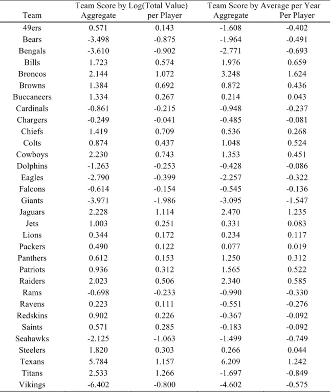
I ran two regressions, both control for all of our variables we previously found as relevant, and both include 31 total dummy variables, one for each team with the Jaguars omitted to ovoid problems with colinearity. I then regressed that set of independent variables on Log(Total Value) and AverageperYear. I highlighted any teams whose
55 https://grades.profootballfocus.com/#/ratings/positions/show/C [11]