MŰHELYTANULMÁNYOK DISCUSSION PAPERS
INSTITUTE OF ECONOMICS, HUNGARIAN ACADEMY OF SCIENCES
MT-DP – 2009/23
A BANKING EXPLANATION OF THE
US VELOCITY OF MONEY: 1919-2004
ISBN 978 963 9796 81 2 ISSN 1785 377X
Discussion papers MT-DP – 2009/23
Institute of Economics, Hungarian Academy of Sciences
KTI/IE Discussion Papers are circulated to promote discussion and provoque comments. Any references to discussion papers should clearly state that the paper is preliminary.
Materials published in this series may subject to further publication.
A Banking Explanation of the US Velocity of Money: 1919-2004
Authors: Szilárd Benk
economist
Economic Analysis and Research Magyar Nemzeti Bank Email: [email protected]
Max Gillman research associate
Institute of Economics - Hungarian Academy of Sciences E-mail: [email protected]
Michal Kejak Associate Professor
The Center for Economic Research and Graduate Education of Charles University (CERGE EI)
E-mail: [email protected]
Az Egyesült Államok 1919 és 2004 közötti pénzforgási
sebességének banki megközelítés
ű
magyarázata
BENK SZILÁRD - MAX GILLMAN - MICHAL KEJAK
Összefoglaló
A tanulmány azt mutatja be, hogy az Egyesült Államokban az 1919 és 2004 közötti időszakban az M1 forgási sebessége átlagosan évi 1,25%-kal növekedett hosszú ciklusokban. A forgásisebesség-ciklusokat egy DSGE-modellből vett sokkokkal, valamint éves adatokkal (Ingram et al., 1994) magyarázza. A modellezett forgási sebesség stabil az endogén növekedésű
és a cserét meghitelező decentralizált banki tevékenységgel jellemzett egyensúlyi növekedési pálya mentén. A hitel termelékenységének és a pénzkínálatnak pozitív sokkja növeli a forgási sebességet, mivel csökken a pénzkereslet; valamint a pozitív árutermelékenységi sokk hatására átmenetileg emelkedik a termelés és a forgási sebesség.
A tanulmány elemzi a forgási sebesség volatilitását üzleti ciklusokon belül, valamint hosszú távon is. A harmincas évektől kezdődően tapasztalt, majd az 1987-es válság idején, továbbá 2003-ban megismétlődött filterezett negatív forgási sebesség azt a felvetést támasztja alá, hogy a pénz- és hitelsokkoknak nagyobb a hatása a forgási sebességre instabil gazdasági időszakokban, míg az árutermelékenységi sokk hatása stabil gazdasági időszakokban jelentősebb.
Tárgyszavak: üzleti ciklus, hitelsokkok, forgási sebesség, volatilitás
CEPR Discussion Paper No. 7544
November 2009
ABSTRACT
A Banking Explanation of the US Velocity of Money: 1919-2004
The paper shows that US GDP velocity of M1 money has exhibited long
cycles around a 1.25% per year upward trend, during the 1919-2004 period. It
explains the velocity cycles through shocks constructed from a DSGE model
and annual time series data (Ingram et al., 1994). Model velocity is stable
along the balanced growth path, which features endogenous growth and
decentralized banking that produces exchange credit. Positive shocks to credit
productivity and money supply increase velocity, as money demand falls,
while a positive goods productivity shock raises temporary output and velocity.
The paper explains such velocity volatility at both business cycle and long run
frequencies. With filtered velocity turning negative, starting during the 1930s
and the 1987 crashes, and again around 2003, results suggest that the money
and credit shocks appear to be more important for velocity during less stable
times and the goods productivity shock more important during stable times.
JEL Classification: E13, E32 and E44
Keywords: business cycle, credit shocks, velocity and volatility
Szilárd Benk
Economist
Economic Analysis and Research
Magyar Nemzeti Bank
Szabadsag ter 8-9
H-1054 Budapest
HUNGARY
Email: [email protected]
For further Discussion Papers by this author see:
www.cepr.org/pubs/new-dps/dplist.asp?authorid=165171
Max Gillman
Cardiff Business School
Cardiff University
Office P01
Colum Drive
Cardiff, CF10 3EU
UK
Email: [email protected]
For further Discussion Papers by this author see:
Michal Kejak
CERGE-EI
Politickych veznu 7
CZ-11121 Prag 1
CZECH REPUBLIC
Email: [email protected]
For further Discussion Papers by this author see:
www.cepr.org/pubs/new-dps/dplist.asp?authorid=132704
Submitted 30 October 2009
The publication of this Paper is funded by the Euro Area Business Cycle
Network (www.eabcn.org). This Network provides a forum for the better
understanding of the euro area business cycle, linking academic researchers
and researchers in central banks and other policy institutions involved in the
empirical analysis of the euro area business cycle. We are grateful to the
referees for excellent critiques and to Jim Bullard for useful comments
1
Introduction
Ireland (1994) modeled the interesting idea that the velocity of money could rise forever, until money was no longer being used, due to continuous techno-logical progress that lowers the cost of credit. This is also the argument that Woodford (2003) makes for why it makes sense to consider monetary policy in an economy without money, the main paradigm of his highly in‡uential work. And this is followed up by Gali (2008), in which money demand plays no role except to equilibrate the money supply as determined residually by the Taylor rule. Hromcova (2008) novelly reformulates the Ireland possibility of an ever rising velocity by using a human capital externality to lower the cost of credit.
Hromcova (2008) uses a Lucas (1988) type endogenous growth economy with human capital and an exchange technology that allows either cash or costly credit use, across a continuum of stores, similar to the cash-credit mix in Gillman (1993) and Ireland (1994). However the cost of credit use is de…ned so that it falls continually as the human capital level in the economy increases. The consumer naturally chooses more credit use over time, and so velocity increases, and the balanced path equilibrium is de…ned as one in which velocity rises steadily, towards in…nity.
We follow the same, well-respected, Lucas (1988) endogenous growth ap-proach, which has support going back to Kocherlakota and Source (1996), however in the form without any human capital externalities which are known to give rise to multiple or indeterminate equilibria. Our cost of credit is not postulated in a general transaction cost form, as in Hromcova (2008), Schmitt-Grohe and Uribe (2004), or as in Bansal and Coleman (1996). Rather it is derived from an equilibrium where credit is produced by an in-dustry -based banking sector with constant returns to scale technology as in Clark (1984). With shocks to credit sector productivity, along with the money supply and goods sector productivity shocks as in the monetary real business cycle (RBC) approach, this economy has a well-de…ned balanced growth path (BGP) equilibrium with a stationary velocity, and not one ris-ing forever (Section 2). Our contribution is then to use this baseline model to explain cycles of the US M1 velocity over a long historical period, with an extension to the UK money velocity for post-1978 data.
Simulations of the model show a good ability to replicate business cycle correlations, both real and "monetary", while explaining 87% of the relative
0% 5% 10% 15% 20% 25% 30% 1919 1923 1927 1931 1935 1939 1943 1947 1951 1955 1959 1963 1967 1971 1975 1979 1983 1987 1991 1995 1999 2003 0.0 1.0 2.0 3.0 4.0 5.0 6.0 7.0 8.0 9.0 10.0 Volatility(Velocity) Velocity (rhs)
Figure 1: Income Velocity Level and its Volatility [Velocity (nominal
GDP=M1). Volatility is de…ned as the standard deviation over a 7-year mov-ing window]
volatility of the M1 income velocity (Section 3). In the Figure 1 graph of US M1 income velocity and its volatility, the data shows a 1.25% average annual upwards trend in the 1919-2004 velocity; in the analysis we use an 86 year Christiano and Fitzgerald (2003) …lter to detrend the data mini-mally to achieve stationarity while leaving in all but the very long run trend component of the data. A decomposition of the velocity volatility provides estimates of the contribution to volatility by each of the three shocks, across various subperiods, and within both business cycle and long run windows. The shocks are constructed from actual annual time series data for the choice variables using the model’s equilibrium solution, following the methodology of Ingram, Kocherlakota, and Savin (1994). In this way the selected group of theoretically plausible RBC style shocks are "backed-out" of the model as in our previous work (Benk, Gillman, and Kejak 2005, Benk, Gillman, and Kejak 2008) and in Nolan and Thoenissen (2009), while constructed so as to have zero mean over the sample period. The paper also illustrates a graphical way to see how the shocks "add up" to explain the velocity cycles over the sample period, and discusses both volatility and level results for the US (Section 4), with extension to the UK (Section 5), and with literature comparison (Section 6).
2
The Model
The representative agent economy is extended from the stochastic shock framework of Benk, Gillman, and Kejak (2008) by decentralizing the bank sector that produces credit; this decentralization follows that of Gillman and Kejak (2009), although there the economy is deterministic. By combining the business cycle with endogenous growth, stationary in‡ation lowers the output growth rate as supported empirically for example in Gillman, Har-ris, and Matyas (2004) and Fountas, Karanasos, and Kim (2006). Over the business cycle, shocks cause changes in growth rates and in stationary ratios. The shocks to the goods sector productivity and the money supply growth rate are standard, while the third shock to the credit sector productivity exists by virtue of the model’s endogeneity of money velocity via a micro-evidence based (Hancock 1985) constant-returns-to-scale (CRS) production of exchange credit as in Clark (1984). This credit technology allows for a unique equilibrium between money and credit use even though they are per-fect substitutes in exchange for the consumer; by including the deposited funds as an "additional factor" of production this gives a rising marginal cost per unit of deposits that equals the marginal cost of money: the nomi-nal interest rate.1
The shocks occur at the beginning of the period, observed by the con-sumer before the decision process, and follow a vector …rst-order autoregres-sive process. For goods sector productivity, zt; the money supply growth
rate, ut;and bank sector productivity, vt:
Zt = ZZt 1+"Zt; (1)
where the shocks are Zt = [zt ut vt]0, the autocorrelation matrix is Z =
diagf'z; 'u; 'vg with 'z; 'u; 'v 2(0;1)as autocorrelation parameters, and the shock innovations are "Zt = [ zt ut vt]0 N(0; ): The general
struc-ture of the second-order moments is assumed to be given by the variance-covariance matrix ; with standard deviations of z, u, and v: These shocks a¤ect the economy as described below.
1Solving this equilibrium problem is discussed as far back as King and Plosser (1984).
Both English (1999) and Gillman (2000), for example, have decentralized bank sectors based on a cash constraint over a goods continuum as in Gillman (1993), with related transaction cost technologies. These have unique money/credit equilibria, but not bank production functions as in Clark (1984). Gillman and Kejak (2004) have a related sec-toral bank decentralization but leave implicit the role of deposits. Without explicit bank deposits, these papers miss how bank pro…t equals the interest return to deposits.
A representative consumer has expected lifetime utility from consumption of goods, ct; and leisure,xt;with 2(0;1)and >0; this is given by
U =E0 1 X t=0 t(ctxt)1 1 : (2)
Output of goods,yt, and increases in human capitalht, are produced with
physical capitalktand e¤ective labor each in Cobb-Douglas fashion; the bank
sector produces exchange credit using labor and deposits dt as inputs. Let
sGt andsHt denote the fractions of physical capital that the agent uses in the
goods production (G) and human capital investment (H), whereby
sGt +sHt = 1: (3)
The agent allocates a time endowment of one amongst leisure, xt; labor
in goods production, lGt, time spent investing in the stock of human capital,
lHt, and time spent working in the bank sector (Q), denoted bylQt:
lGt+lHt+lQt+xt = 1: (4)
Output of goods can be converted into physical capital, kt; without cost
and so is divided between consumption goods and investment, denoted by
it; gross of capital depreciation, where the depreciation rate is K 2 [0;1].
Thus, the capital stock used for production in the next period is given by:
kt+1 = (1 K)kt+it= (1 K)kt+yt ct: (5)
The human capital investment is CRS-produced using capital sHtkt and
ef-fective labor ntht :
H(sHtkt; lHtht) = AH(sHtkt)1 (lHtht) : (6)
And the human capital ‡ow constraint, with depreciation rate H 2 [0;1];
is:
ht+1 = (1 H)ht+H(sHtkt; lHtht): (7)
Withwtandrtdenoting the real wage and real interest rate, the consumer
receives nominal income of wages and rents, Ptwt(lGt+lQt)ht andPtrtsGtkt;
a nominal transfer from the government, Tt; and dividends from the bank.
The consumer buys shares in the bank by making deposits of income at the bank. Each dollar deposited buys one share at a …xed price of one,
and the consumer receives the residual pro…t of the bank as dividend income in proportion to the number of shares (deposits) owned. Denoting the real quantity of deposits by dt;and the dividend per unit of deposits asRQt; the
consumer receives a nominal dividend income ofPtRQtdt:The consumer also
pays to the bank a fee for credit services, whereby one unit of credit service is required for each unit of credit that the bank supplies the consumer for use in buying goods. With PQt denoting the nominal price of each unit of
credit, andqtthe real quantity of credit that the consumer uses in exchange,
the consumer pays PQtqt in credit fees and buys Ptqt in goods with credit.
With total goods expenditures,Ptct;physical capital investment,Ptkt+1
Pt(1 K)kt;and investment in cash for purchases,Mt+1 Mt;the consumer’s
budget constraint is
Ptwt(lGt+lQt)ht+PtrtsGtkt+PtRQtdt+Tt (8)
PQtqt+Ptct+Ptkt+1 Pt(1 K)kt+Mt+1 Mt:
The consumer can purchase the goods by using either moneyMtor credit
services. With the lump sum transfer of cashTtcoming from the government
at the beginning of the period, and with money and credit equally usable to buy goods, the consumer’s exchange technology is
Mt+Tt+Ptqt Ptct: (9)
Since all cash comes out of deposits at the bank, and credit purchases are paid o¤ at the end of the period out of the same deposits, the total deposits are equal to consumption. This gives the constraint that
dt=ct: (10)
The bank produces credit that is available for exchange at the point of purchase. The bank determines the amount of such credit by maximizing its dividend pro…t subject to the labor and deposit costs of producing the credit. The production of credit uses a constant returns to scale technology with e¤ective labor and deposited funds as inputs (physical capital is omitted as a factor for simplicity). This follows the "…nancial intermediation approach" (Matthews and Thompson 2008) that is dominant in the banking literature, which was started by Clark (1984). In particular, withAQ >0and 2(0;1);
qt =AQevt(lQtht) d1t ; (11)
where AQevt is the stochastic factor productivity.2
Subject to the production function in equation (11), the bank maximizes pro…t Qt with respect to the labor ft and deposits dt:
Qt =PQtqt PtwtlQtht PtRQtdt: (12)
Equilibrium implies that
PQt Pt = wt AQevt lQtht dt 1; (13) PQt Pt = RQt (1 )AQevt lQtht dt : (14) Equations (13)-(14) indicate that the marginal cost of credit PQt
Pt equals the marginal factor prices divided by the marginal factor products:
The …rm maximizes pro…t t, given by t=yt wtlGtht rtsGtkt;subject
to a King and Rebelo (1990) technology in e¤ective labor and capital:
yt=AGezt(sGtkt)1 (lGtht) : (15)
The …rst order conditions for the …rm’s problem are
wt= AGezt sGtkt lGtht 1 ; (16) rt= (1 )AGezt sGtkt lGtht : (17)
2This "banking time" model can be interpreted as a special case of the shopping
time model: substituting qt from equation (11) into equation (9), and for dt from equa-tion (10), and solving for the e¤ective banking time as lQtht = ct
Mt+1 Pt AQevtc1t 1= ; then lQtht = g(Mt+1
Pt ; ct); with g1 < 0 and g2 > 0; as in a shopping time model. However there is no Feenstra (1986) equivalence to a standard money-in-the-utility function model in that ht would enter the utility function, as seen by solving for the raw bank time
lQt=g MPt+1t ; ct =ht;substituting forlQtin the allocation of time constraint (4), solving
It is assumed that the government policy includes sequences of nominal transfers which satisfy:
Tt= tMt = ( +eut)Mt; t= [Mt+1 Mt]=Mt: (18)
where t is the growth rate of money and is the stationary growth rate
of money.
The equilibrium can be de…ned by writing the representative agent’s op-timization problem recursively as:
V(s) = max c;x;lG;lH;lQ;sG;sH;q;d;k0;h0;M0 ( cx 1 1 + EV(s 0) ) (19) subject to the conditions (3) to (10), where the state vector of the economy is denoted by s = (k; h; M; z; u; v) and a prime (’) indicates the next-period values. A competitive equilibrium consists of a set of policy functions c(s),
x(s), lG(s),lH(s), lQ(s),sG(s), sH(s); q(s),d(s), k0(s),h0(s), M0(s), pricing
functions P(s), w(s), r(s); RQ(s); PQ(s); a transfer function T(s); a value
function V(s), and initial conditions k0, h0; M0 such that
(i) givens; P(s),w(s),r(s); RQ(s); PQ(s);and T(s);the consumer solves
the optimization problem in equation (19);
(ii) givens; P(s), w(s), RQ(s); and PQ(s), the bank maximizes pro…t in
(12) subject to equation (11);
(iii) given s; P(s), w(s), r(s) the goods producer maximizes pro…t; (iv) the goods, money and credit markets clear, in equations (5), (9), (11), (15) and (18).
2.1
Balanced-Growth Path Equilibrium
As derived from the equilibrium above (see Appendix A.4 for the …rst-order conditions), a partial set of equilibrium conditions along the balanced-growth path (BGP) are given here to describe the deterministic balanced-growth path equilibrium, and how in‡ation a¤ects it. The balanced-growth rate is denoted by g; with ct; kt; ht, qt; dt; and MPt+1t all growing at the rate g;
nominal prices grow at the stationary in‡ation rate denoted by :Dropping time subscripts on stationary variables, the BGP conditions include :
1 + PQt
Pt
x ct = 1 +R wht ; (21) R= 1 qt dt R+ qt dt R; (22) qt dt = (AQ) 1 1 R w 1 ; (23) rH AH sHkt lHht (1 ) (1 x); (24) (1 +g) = (1 +rH H) = (1 +r K): (25)
The solution for consumption-normalized money demand (inverse veloc-ity), 1 qt
ct; is derived from equation (9), (10) and (23); the consumption velocity of money, denoted by Vct; is given by
Vct ct Mt+1 Pt = 1 1 qt ct : (26)
This rises at an increasing rate as the nominal interest rate rises. In particu-lar, the interest elasticity of normalized money,
Mt+1 Pt ct ;is equal to qt dt 1 qt ct (1 ) ;
and this rises in magnitude as the interest rate increases and causes more credit use. The relative price of credit PQt
Pt equals its marginal cost and by equation (20) this equals the nominal interest rate R. At the …rst best op-timum, R equals zero and no credit is used. As in‡ation rises, the agent substitutes from goods towards leisure while equalizing the margin of the ratio of the shadow price of goods to leisure, x=( ct) =
h
1 +Ri=(wht); in
equation (21). HereR;as given in equation (22), is the average exchange cost per unit of output; this equals the average cost of using cash, R; weighted by 1 qt
dt and the average cost of using credit, R; weighted by
qt
dt: Equa-tion (23) gives the soluEqua-tion for qt
dt; and in turn velocity (equation 26), from equations (11), (13), and (20) (the dividend rate RQt follows from equation
14). Equations (24) and (25) indicate the subsequent growth e¤ects that are important in identifying the money and credit shocks within the endoge-nous growth framework. In‡ation-induced increases in leisure decrease the human capital return of equation (24), and lower the growth rate in equation (25). The use of more credit to avoid in‡ation instead of using leisure means that leisure increases by less and the growth rate falls by less (Gillman and
Kejak 2005). Therefore a shock to the money supply causes higher in‡ation, more credit use, less money demand, higher velocity and less growth. If such higher in‡ation and increased credit use are correlated with productivity in-novation in the credit sector, then this leads to a high correlation between the money and credit productivity shocks as identi…ed by the model.
2.2
Exogenous Growth
For comparison, a way of introducing exogenous growth is by letting human capital follow the exogenous trend given by g : ht+1 = ht(1 +g); and with
lHt = sHt = 0. As in endogenous growth, the sectoral productivity
para-meters AG and AQ are constant and also both the income and consumption
velocities of money are constant along the BGP, while all growing variables grow at the same rate of g:
3
Model Simulation
By normalizing the variables that grow along the deterministic steady state, and then log-linearizing the all model equilibrium conditions around this normalized deterministic steady state, we get a stochastic linear system of equations. Here we normalize by dividing by the human capital stockht:This
system of equations is in terms of kt=ht and the three shocks; it is solved by
using standard techniques as in Hartley, She¤rin, and Salyer (1997).
3.1
Calibration
Table 1 presents the parameters for the calibration which are chosen in order to match the Table 2 target values that are average annual values from US time series for 1919-2004 and that re‡ect issues raised by Gomme and Rupert (2007), in their two-sector RBC model; our human capital sector is a related second sector. The capital share in the goods sector is set at 1 = 0:36
as in Jones, Manuelli, and Siu (2005), the annual discount factor is set at
= 0:96, and log-utility is assumed so that = 1: The US average annual output growth rate g is set at 2:4% as in the data. The baseline investment to output ratio target value is i=y = 0:26; implying the annual depreciation rate K = 0:031 and the real interest rate net of depreciation of r K =
0:067:3 The rate of depreciation of human capital is set at
H = 0:025; as in
Jones et al. (2005) and Jorgenson and Fraumeni (1989). The allocation of time is similar to Gomme and Rupert (2007), with the working time set at
lG = 0:2482 and leisure at x = 0:55. Time in human capital investment is
set at lH = 0:2. Given lH; g; and H implies the capital to e¤ective labor
ratio in the human capital sector, its capital share of = 0:83; and in turn an AH = 0:21 and a leisure utility weight of = 1:84:
In the banking sector we set the value of the inverse of the consumption velocity of M1 money, M=(P c), equal to the average annual value for the period 1919-2004, which is 0.38. The average annual in‡ation rate, , over the same period is 2.6% which implies that the annual money growth is equal to 5%. Using an approximate cost of an exchange credit card (American Express) at $100, and the per capita annual consumption expenditure, c=
$15780, both at 2006 prices, the share of the labor in the banking sector
is = 100=[Rc(1 [M=(P c)])] = 0:11: A similar calibration of this labor
share is made in Benk et al (2008). It implies that only 11% of the interest return R is used up in the process of producing the exchange credit, which is a result focused on in Gillman and Kejak (2009). And it follows that the marginal cost per unit of credit is an upward sloping, and for any < 0:5;
convex curve; so with this calibration the supply curve has its typical shape of a marginal cost rising at an increasing rate.
Table 1 also includes the parameters characterizing the shock processes of equation (1); these are chosen through an iterative process by which the assumed shock parameters converge with the actual shock parameters that are in turn estimated from the constructed shock processes described in Ap-pendix A.1. In particular, estimated parameters are inputted back into the model, shocks are re-constructed and parameters re-estimated until conver-gence is achieved in the parameter structure. For comparison, the exogenous growth version of the model without human capital investment assumes the same parameters as those used for the baseline endogenous growth model, except that the target labor time lG increases to include the targeted time
lH in human capital investment.
3For comparisoni=y= 0:13in Gomme and Ruppert (2007) for postwar market
struc-tures, equipment and software; including their consumer durables increases this by0:10;
Preferences
1 Relative risk aversion parameter 1.84 Leisure weight
0.96 Discount factor
Goods Production
0.64 Labor share in goods production
K 0.031 Depreciation rate of goods sector
AG 1 Goods productivity parameter
Human Capital Production
0.83 Labor share in human capital production
H 0.025 Depreciation rate of human capital sector
AH 0.21 Human capital productivity parameter
Banking Sector
0.11 Labor share in credit production
AQ 1.1 Banking productivity parameter
Government
0.05 Money growth rate Shocks processes
Autocorrelation parameters
'"z 0.84 Production productivity
'u 0.74 Money growth rate
'v 0.73 Banking productivity Standard Deviation of Shock Innovations
z 0.77 Production productivity u 0.50 Money growth rate v 1.16 Banking productivity
Table 1: Parameters of Calibration
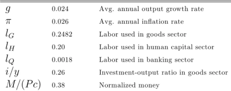
g 0.024 Avg. annual output growth rate 0.026 Avg. annual in‡ation rate
lG 0.2482 Labor used in goods sector
lH 0.20 Labor used in human capital sector
lQ 0.0018 Labor used in banking sector
i=y 0.26 Investment-output ratio in goods sector
M=(P c) 0.38 Normalized money
0 50 0 1 2 PR to vel 0 50 0.5 1 1.5 M to vel 0 50 0.2 0.4 0.6 0.8 1 CR to vel
Figure 2: Impulse Responses of Income Velocity of Money
0 50 1.35 1.4 1.45 1.5 CR to vel 0 50 1.3 1.4 1.5 1.6 PR to vel 0 50 1.35 1.4 1.45 1.5 1.55 M to vel
Figure 3: Transition Dynamics of Income Velocity of Money
3.2
E¤ect of Shocks on Velocity
Figure 2 illustrates the impulse responses of income velocity (vel in …gure) when faced with a temporary 1 % increase in the credit shock (CR), goods productivity shock (PR), and money shock (M). All three shock cause ve-locity to rise initially, with a gradual decrease back to equilibrium for the credit and money shocks, and some decrease in velocity from the PR shock after the initial increase. The productivity shock increases velocity mainly by increasing temporary output; velocity falls after a while, before returning to the original equilibrium, as the increased goods productivity decreases the price of goods relative to labor, so that in‡ation decreases and money de-mand increases. The money shock causes a jump in the price level, in‡ation, and interest rates and decreases real money demand; the credit shock makes the marginal cost of credit lower, inducing a decrease in money demand and an increase in credit use.
Consider in contrast when there is a shock that does not dissipate, so that the shock is permanent, and then velocity transitions from one BGP to another one. Assuming a 10% permanent increase in each of the three shock variables, Figure 3 shows the original (dashed line) BGP equilibrium and the movement to the new BGP equilibrium (solid line). The …gure shows the
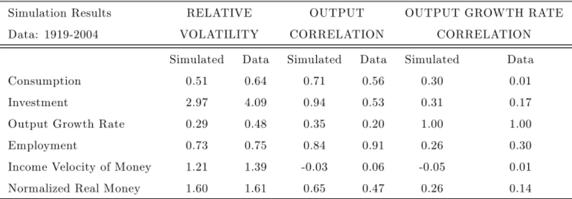
Simulation Results RELATIVE OUTPUT OUTPUT GROWTH RATE Data: 1919-2004 VOLATILITY CORRELATION CORRELATION
Simulated Data Simulated Data Simulated Data Consumption 0.51 0.64 0.71 0.56 0.30 0.01 Investment 2.97 4.09 0.94 0.53 0.31 0.17 Output Growth Rate 0.29 0.48 0.35 0.20 1.00 1.00 Employment 0.73 0.75 0.84 0.91 0.26 0.30 Income Velocity of Money 1.21 1.39 -0.03 0.06 -0.05 0.01 Normalized Real Money 1.60 1.61 0.65 0.47 0.26 0.14
Note: See Appendix for data sources. All data series represent the cyclical component of the data …ltered with the Christiano and Fitzgerald (2003) asymmetric frequency …lter with a band of 2-86 years (86=sample size). Series are in logs except those that represent rates. Relative volatility is measured as
the ratio of standard deviation of the series to the standard deviation of GDP
Table 3: US Business Cycle Facts, 1919-2004, and Simulations
goods sector shocks causes income velocity to initially increase and then fall down to a new lower steady state, while the money and credit shocks cause velocity to rise with virtually no transition dynamics. The goods sector shock causes income to rise initially while prices are gradually decreased; with less in‡ation, more money is used and income velocity eventually falls. The money shock simply makes in‡ation higher and increases velocity, while the credit shock makes credit less expensive and so decreases money demand and increases velocity.
3.3
Simulations
Table 3 presents US data (see Appendix A.3) stylized facts and model sim-ulations, in terms of moments of a set of variables for the period 1919-2004, where the data series have been detrended using the Christiano and Fitzger-ald (2003) asymmetric frequency …lter with a band of 2-86 years (where 86 is the sample size). And in the simulations, the Consumption and Investment level variables are normalized by human capital. The table shows that simu-lated relative volatilities of consumption and investment ratios are 0.51 and 2.97, compared to data of 0.64 and 4.09. Output growth volatility is 0.29 compared to 0.48 for GDP data. And simulated consumption and investment correlation with output is 0.71 and 0.94 versus 0.56 and 0.53 in the data.
of money is 1.21 as compared to 1.39 in the data, which means the model explains 87% of the volatility found in the GDP velocity of M1 that exists in the data. The normalized real money volatility is 1.60, almost identical to 1.61 in the data. The income velocity’s correlation with output is -0.03, compared to the data’s 0.06. Real money correlation with output is 0.65 compared to the data value of 0.47; and with output growth it is 0.26 versus 0.14. Not shown, the simulated correlation of in‡ation with money growth is 0.49, as compared to 0.42 in the data.
4
Decomposing the E¤ect of Shocks on
Ve-locity
We construct the shocks by adapting the methodology of Ingram et al (1994) for this endogenous growth model, a procedure described in Benk et al. (2008). Here we solve the equilibrium solution for each control variable as a function of the endogenous state variable and the three shocks, gather time series for a set of choice variables and use this data to solve for each shock at each timet; please see Appendix A.1. With three such time series the shocks are exactly identi…ed. We use more than three series to base the shocks on more information, thereby over-identifying the shocks, and then estimate the shocks using a minimum distance approach, described in Benk et al. (2008). A di¤erence from previous work is that here we use annual data and a band pass …lter that takes out only the 86 year trend, so as to leave in longer run cycles along with business cycles.
4.1
E¤ect on Velocity Levels
The e¤ects of these shocks on the income velocity of money can be devised by decomposing the cyclical component of velocity into the contributions of productivity, money and credit shocks. A linear decomposition can be done by using the solution of the model that writes every model variable as a linear function of the state vector s = (k[t=ht; z; u; v); where for any ;
^ log( ) log( )is the percentage deviation of from its steady state value
: For the income velocity of money, denoted byVt; it follows that :
b Vt d ytPt Mt+1 = kk[t=ht+ zzt+ uut+ vvt+eVt ; (27)
-45% -35% -25% -15% -5% 5% 15% 25% 35% 1919 1921 1923 1925 1927 1929 1931 1933 1935 1937 1939 1941 1943 1945 1947 1949 1951 1953 1955 1957 1959 1961 1963 1965 1967 1969 1971 1973 1975 1977 1979 1981 1983 1985 1987 1989 1991 1993 1995 1997 1999 2001 2003
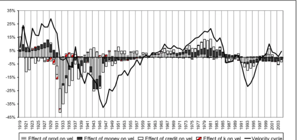
Effect of prod on vel Effect of money on vel Effect of credit on vel Effect of k/h on vel Velocity cycle
Figure 4: E¤ect of Shocks and k=h on US Income Velocity; Endogenous Growth Model, 1919-2004.
where zzt, uut and vvt indicate the contribution of productivity, money
and credit shocks to the cyclical component of velocity.4 Since we use more variables than shocks, the model does not perfectly …t the data series used to construct the shocks, leaving an error term eVt .
Velocity decompositions based on equation (27) are shown in Figure 4, along with the Christiano and Fitzgerald (2003) 86 year detrended velocity itself. Much of the movement of the velocity cycles over time is captured by the shocks of the model, with less success during the 1930s depression and more success since the end of WWII. For example, Figure 4 shows that pro-ductivity shocks contributed to a signi…cant amount of the velocity changes after WWII, but that the money and credit shocks were also important such as during the 1970s in‡ation and the post 2001 velocity movement.
The e¤ect of shocks on the level of …ltered income velocity can also be computed for the exogenous growth version of the model (Figure 5). Com-parison of Figures 4 and 5 gives a distinct sense in which the endogenous growth model is able to explain more of the actual …ltered velocity level than the exogenous growth model. This appears true in the 1920s, from 1939-1959, 1961-1970, and since 1990. The actual shocks of the endogenous growth versus exogenous growth models are compared in Figure 7 in Appen-dix A.1; endogenous growth forces more correlation between the money and
4Fork=hwe are not aware of any human capital estimate back to 1919, and so assume
-45% -35% -25% -15% -5% 5% 15% 25% 35% 1919 1921 1923 1925 1927 1929 1931 1933 1935 1937 1939 1941 1943 1945 1947 1949 1951 1953 1955 1957 1959 1961 1963 1965 1967 1969 1971 1973 1975 1977 1979 1981 1983 1985 1987 1989 1991 1993 1995 1997 1999 2001 2003 Effect of prod on vel Effect of money on vel Effect of credit on vel Effect of k on vel Velocity cycle
Figure 5: E¤ect of Shocks and k=h on US Income Velocity; Exogenous Growth Model, 1919-2004.
credit shocks. There is more "smoothing" for the money shock with exoge-nous growth; and the credit shock behavior during the 1930s di¤ers between the two models.
4.2
E¤ect on Velocity Volatility
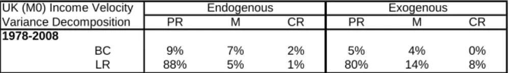
We decompose the ‡uctuations in the cyclical component of the GDP velocity of M1 money (which is from the data) and show how much of the variance is explained within each subperiod by each of the model’s three shocks, the pro-ductivity (PR), money (M) and credit (CR) shocks, and across business cycle (BC) and long run (LR) frequencies such as in Levy and Dezhbakhsh (2003) (see Appendix A.2). With a variation on Ingram et al.(1994), we take an unweighted average over all six possible orderings of the three shocks. Table 4 reports variance decompositions for the entire 2004 period, for 1919-1935 (Roaring 20s-depression), for 1936-1954 (recovery-WWII), for 1955-1982 (postwar and high in‡ation), and for 1983-2004 (Moderation). Here the variance-covariance matrices have been estimated separately for each sub-period so as to obtain simulated series and decompositions that di¤er by subperiods.
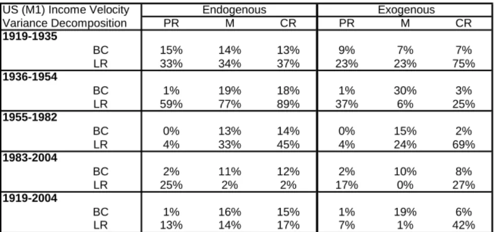
Table 4 shows the US (M1) income velocity variance decomposition re-sults. The columns show the fraction of the data variance, by frequency, that is explained by each shock, for both endogenous and exogenous growth
mod-US (M1) Income Velocity Endogenous Exogenous Variance Decomposition PR M CR PR M CR 1919-1935 BC 15% 14% 13% 9% 7% 7% LR 33% 34% 37% 23% 23% 75% 1936-1954 BC 1% 19% 18% 1% 30% 3% LR 59% 77% 89% 37% 6% 25% 1955-1982 BC 0% 13% 14% 0% 15% 2% LR 4% 33% 45% 4% 24% 69% 1983-2004 BC 2% 11% 12% 2% 10% 8% LR 25% 2% 2% 17% 0% 27% 1919-2004 BC 1% 16% 15% 1% 19% 6% LR 13% 14% 17% 7% 1% 42%
Table 4: Decomposition of Variance of Velocity by Frequency, 1919-2004 els. For example, with endogenous growth, in the subperiod of 1919-1935, the model explains a total of 15+14+13=42% of the actual variance found within the BC frequency, and 33+34+37=104% of the variance within the LR frequency, for a total of 146% of the variance. Therefore the 1919-1935 total model volatility is 46% more than in the data. Similarly the model explains 263% of the volatility for 1936-1954, 109% for 1955-1982, 54% for 1983-2004, and 76% for the whole period, 1919-2004.
The standard deviation and correlation of the shocks di¤er somewhat between the endogenous and exogenous growth versions, for the whole period, and when divided by subperiod (details not reported). Both models have a standard deviation of the productivity shock that drops signi…cantly post 1954. In both models, the standard deviation of the money shock is rather stable across all four subperiods, while the standard deviation of the credit shock is lower in the second two subperiods than the …rst two, as with the goods productivity shock. Focusing on endogenous growth, in the whole 1919-2004 period, the standard deviations are 0.48, 0.28, and 0.68 for P R; M; and CR: And the credit shock standard deviation doubles from 0:21 in 1955-1982 to 0.40 in 1983-2004. In the whole period, the money and credit shocks have a 0.75 correlation, while credit and goods productivity shocks have a -0.51 correlation, and money and goods productivity have a 0.17 correlation. However there is a negative correlation of credit with goods productivity in each of the …rst three subperiods but a positive one during 1983-2004. And money and credit shocks have a high positive correlation (above 0.90) in the latter three subperiods but 0.18 in 1919-1935.
4.3
Discussion of Results
The results show the importance of the contribution of the shocks within the long run frequency, as well as the importance individually of each of the three shocks. A positive goods productivity shock works mainly on the income term in the income velocity of money, by increasing the economy’s temporary output/income. This causes output to rise relative to consumption since consumption follows the permanent income and only increases somewhat when temporary income rises. Therefore the income to consumption ratio rises.
With a standard exchange constraint, and only cash used to buy goods, then the story of income velocity ends with the income to consumption ra-tio since money demand always equals consumpra-tion demand. With credit available, the consumer can substitute away from money towards credit. The money and credit shocks a¤ect this substitution and thereby a¤ect mainly the money to consumption ratio. A positive money shock raises in‡ation and causes substitution towards credit; this shock also decreases the growth rate of income because of the in‡ation tax e¤ect. A positive credit productivity shocks works similarly in that substitution occurs from money to credit, but in reverse has a positive e¤ect on income and its growth rate. The main e¤ect on velocity from the money and credit shocks is the substitution e¤ect rather than the income e¤ect, and both a¤ect velocity similarly in magnitude (as in Figures 2 and 3).
When the productivity shock explains a greater amount of velocity volatil-ity than the money and credit shocks, it means that the period is charac-terized more by simple changes in temporary income that little a¤ect the consumption demand. This type of velocity volatility from goods produc-tivity shocks, is more of the "normal" type associated with the RBC real economy model. However when there are signi…cant variations in the money supply, such as in response to big debt increases from war or bank crises, then there can be more of the traditional monetary type of velocity volatility. And these money shocks either stimulate credit use or credit may be suppressed and cannot respond. In the former case, the velocity rises by more because of both less money and more credit use. If credit is suppressed, such as during the Depression when banks failed, and in the recent bank crises, then velocity volatility would be expected to be explained somewhat more by money than by credit shocks.
4.3.1 US Velocity Volatility
Results show for endogenous growth that money and credit shocks contribute similar amounts to velocity volatility. In the …rst two subperiods before 1955, money contributed marginally more at the business cycle frequency than credit, while in the last two subperiods credit contributed slightly more than money to volatility. This is not inconsistent with credit being more constrained in the …rst two subperiods and less constrained in the second two, when there was steady …nancial innovation as international capital markets expanded after WWII and as deregulation took place in the 1970s and 1980s. The large role of money and credit shocks in the LR frequency indicate that these shocks added up to have an e¤ect of greater permanence than found in the typical business cycle frequency. This can be interpreted as the long run in‡ation tax nature of money shocks being more important than the business cycle e¤ects, all the way from 1919 to 1982. During the 1983-2004 "Moderation" and in‡ation targeting policy, the long term e¤ects of credit and money shocks were not important. Instead the goods productivity e¤ects dominated the long term e¤ects on velocity, in reverse of 1955-1982.
4.3.2 US Velocity Levels
The e¤ect of shocks on the magnitude of …ltered velocity levels shows an additional dimension to the volatility e¤ects. In Figure 4, for example in the 1990s, the level e¤ects are nicely explained by the shocks: during high growth and low in‡ation, velocity levels moved down as explained by goods productivity lowering in‡ation and by money supply policy lowering in‡ation. High credit shock components of velocity at the end of the 1990s and up to 2004 indicate that credit is starting to have a large level e¤ect, while the contribution of goods productivity is receding, a possible warning sign of the ending of the stable period.
Changes in the state variable,k=h (indicated by the red portions on the graph) a¤ect the level of …ltered velocity negligibly post-1955 but signi…cantly pre-1955. The transition dynamics indicate that state variable changes occur mainly from changes in the goods productivity shock, and only slightly from the money and credit shocks (details not shown). This suggests that the high contribution of the state variable to pre-1955 velocity levels is mainly from erratic goods productivity shocks. The lessor e¤ect of the state variable on velocity after 1955 in turn re‡ects how the goods productivity shock is more
stable; indeed the standard deviation of the goods productivity shock falls substantially in the two post-1955 subperiods to 0.07 and 0.11, chronologi-cally, from the two pre-1955 subperiod values of 0.74 and 0.68.
5
Extension to the UK
The analysis can be extended to the UK for a more limited time period. The UK data for the …nancial sector exists starting in 1978, from the O¢ ce for National Statistics, and this determines our period of 1978-2008. Rather than ending at the 2004 moderation end-point, this sample includes moving into the recent bank crises.
The income velocity of the UKM0aggregate increases on average by 2.1% per year over the period, compared to 1.25% average per year increase for the US M1income velocity.5 The calibration of the model is kept similar to the US, except with the money supply growth rate at0:075;in‡ation at0:05;and normalized money at 0:33: The shock processes for this more limited period have higher autocorrelations than for the US, and lower standard deviations.6 The same 2-86 …lter on data is used for more direct comparison, although a 2-31 …lter could also be used and we expect the results to be similar.
Given the greater persistence of the shocks for the UK, the impulse re-sponses for the UK (not shown) re‡ect a slower return to the steady state. The actual computed shocks (not shown) are positively correlated at 0.89 be-tween money and credit shocks, 0.94 bebe-tween money and goods productivity shocks, and 0.73 between credit and goods productivity shocks. The goods productivity shock goes from a positive value to becoming steadily negative after 2001 for the endogenous growth model. The credit productivity shock also turns slightly negative around that time, while the money shock is more correlated with the goods productivity shock.
Figure 6 for the endogenous growth model shows that the model seems
5M0 is used as the money aggregate in the data used to construct the shocks for the
UK, and the cyclical component ofM0 income velocity of money is graphed in Figure 6. The UKM1 aggregate includes overnight deposits of banks that are much higher propor-tionately than in the US or the Euro area, makingM1not so comparable to the broader US monetary aggregates. With the UK money to consumption ratios of the aggregates for the period 1978-2008 beingM0=(P c) = 0:06,M1=(P c) = 0:78,M2=(P c) = 1:27, and
M4=(P c) = 1:24;we use an intermediate value betweenM0 and M1 ofM=(P c) = 0:33
for the UK calibration, which is close to the US value ofM=(P c) = 0:38: 6These are('
-45% -35% -25% -15% -5% 5% 15% 25% 35% 45% 1978 1980 1982 1984 1986 1988 1990 1992 1994 1996 1998 2000 2002 2004 2006 2008 Effect of prod on vel Effect of money on vel Effect of credit on vel Effect of k/h on vel Velocity cycle
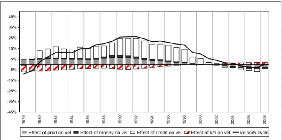
Figure 6: E¤ect of Shocks on UK Income Velocity; Endogenous Growth Model, 1978-2008.
to capture the level of the …ltered UK M0 income velocity well, while the exogenous growth model does not appear to explain the velocity as well (not shown), just as with the US results. Table 5 shows that most of the volatility of the income velocity is explained by the productivity shock in the LR part of the spectrum, and that money plays the next biggest role in explaining volatility.
Comparison of the UK and US endogenous growth results can best be made for the similar periods of 1983-2004 for the US and 1978-2008 for the UK. The productivity shock in both countries during this time plays the biggest role in explaining velocity volatility, while the credit shock contributes more to the volatility in the US than in the UK. For both the US and UK the goods and credit productivity shocks show up signi…cantly in a¤ecting the level of velocity, in Figures 4 and 6. This suggests that the credit shock has been important for both US and UK but more stable in the UK. The UK-US results, for the similar time periods, support the interpretation that "normal" goods productivity e¤ects explain most of the volatility, rather than the money and credit e¤ects as in earlier periods in the US. But at the same time, the drop o¤ of the positive credit shocks and the downturn in …ltered velocity, from 2000-2003 for the US and for 2001-2007 for the UK, indicate potential economy-wide fragility. With hindsight it can be postulated that these credit shocks as seen through velocity were precursors to the ensuing 2007-2009 credit crises: consider that related credit shock and …ltered velocity
UK (M0) Income Velocity Endogenous Exogenous Variance Decomposition PR M CR PR M CR 1978-2008
BC 9% 7% 2% 5% 4% 0% LR 88% 5% 1% 80% 14% 8%
Table 5: Decomposition of Variance of Velocity by Frequency, UK patterns emerge before the troughs of the US 1930s depression and the US 1987 recession. In fact, US …ltered velocity turned negative in the 30s, again in 1986-87, and approached this in 2003; and this happens in the UK in 2004.
6
Comparison to Literature
Ingram et al.(1994) show that the variance decomposition of the goods pro-ductivity shock is not unique but rather depends upon the ordering of the shocks. We verify that result by considering all possible shock orderings, and since there is no obvious rationale for ordering one shock ahead of another, an average is taken across all orderings. Our work is relatively novel in that the shocks considered are the "standard" monetary RBC shocks of goods produc-tivity and money, plus a more novel shock to the credit sector producproduc-tivity. This directly extends the Cooley and Hansen (1989) work to when velocity is endogenous, while using this exciting shock construction technique of Ingram et al, in which the world as we know it is the model, and given this, these are the shocks of this world. Plausibility requires that the exchange credit shock is based in a realistically endogenous velocity. The production of ex-change credit using the empirically robust Clark (1984) production function provides such a plausible endogenous velocity instead of using the standard cash-only consumption velocity of unity; this makes it a reasonable basis for the credit shock that a¤ects velocity. Although such a credit shock is novel to our own work, a related approach is used in Nolan and Thoenissen (2009). They also have standard goods productivity and money supply shocks, and a third, novel, credit shock. Their alternative credit shock is based in a …-nancial accelerator model, and so is more of an intertemporal credit shock rather than the exchange credit shock of this paper. But as in Ingram et al. and this paper, they also back out the shocks using the same methodology. They show how their credit shock is an interesting indicator of economic downturns.
with this methodology, using a plausible credit shock, and its goal is to show that analysis of the identi…ed shocks o¤ers a way to better understand not just velocity per se but also how velocity foreshadows economic crises, especially bank related crises. It is staking out the case that velocity matters not only as another aspect of the long cyclic experience that a good model should be able to explain in conjunction with other "real" aspects, but also as a possible harbinger of crisis that consequently warrants further study.
Finally, our …ltering methodology of including the long run frequency in the data as well as the business cycle frequency is novel in this context and indicates how models that endogenize growth over time may be the best route towards understanding the e¤ect of both the long lasting shocks that indeed should a¤ect growth, as well as those shocks that are more de…ned at business cycle frequencies during which exogenous growth assumptions may be more innocuous.
7
Conclusion
The paper explains US velocity cycles around its 1.25% trend in terms of historically constructed money, credit and goods productivity shocks under endogenous growth. The results show how a signi…cant proportion of the volatility of (86-year band-pass …ltered) velocity can be explained with these shocks, in both business cycle and long run frequencies. Applying the model also to the UK for 1978-2008 supports features seen during the US in the 1983-2004 moderation period, such as stable economic periods coinciding with velocity volatility being explained mainly by the goods productivity shock. An interpretation is that as money supply policy ‡uctuations are stabilized, such as with in‡ation targeting at low levels of the in‡ation rate, there is less of a need to use variations in credit to avoid variations in in‡a-tion, leaving only normal ‡uctuations in temporary income from the goods productivity shock to a¤ect velocity volatility. During more unstable periods of monetary policy, the money and credit shocks can swamp the e¤ect of the goods productivity shocks and explain more of the velocity variation. Given the correlation amongst the identi…ed shocks, it is also plausible that more variable money and credit shocks themselves lead to more variable goods productivity shocks.
Understanding velocity volatility provides another dimension, or re‡ec-tion of activity if you will, that helps explain how we get more stable periods
of aggregate activity, such as after 1982. Conjecturing from here towards recent policy experience, this suggests that the US sustained low nominal in-terest rate policy of 2002-2004, and of 2008 onwards, may be cases described by Friedman (1968) of trying to peg low real interest rates that lead to new eras of unwanted ‡uctuations in government debt, money supply, and private credit. When huge debt build-ups occur, such as during the current bank crisis, then the dominance of goods productivity shocks will likely recede as money and credit shocks again take over in importance in explaining velocity. And should this occur, as it seems it is now likely, it portends the advent of greater in‡ation and even output volatility.
For monetary policy, a "state-dependent" money supply rule that o¤sets velocity changes in order to target in‡ation, as in McCallum (1990) and Keynes (1923), could be directed at the band-pass …ltered velocity. Such a policy in the US historical sample here would have raised money supply growth substantially during the 1930s depression, the 87 stock crash, the 1991 recession and at the end of the sample in 2004 and beyond, in that …ltered velocity has continued to fall. Unlike Taylor interest rate rules with issues of a zero nominal bound, this policy rationalizes the current US policy of "quantitative easing" that involves dramatically increasing the money supply growth rate.
A
Appendix
A.1
Shock ConstructionIn this approach we used six variables to construct the economy’s three shocks, shown in Figure 7, as opposed to …ve variables in Benk et al. (2008), and with the additional variable being the in‡ation rate (others areM=(P y),c=y; i=y,lQand
the wage rate in banking as a proxy for the marginal product of labor in banking). Using data series on these six variables and computed series on the endogenous state variable,k=h; the three shocks are then identi…ed using a minimum distance approach as in Benk et al. (2008). For robustness, the shock construction is repeated for six variables taken …ve at a time, four at a time, and three at a time (exact identi…cation). Nearly the same shock series results for all combinations that include , M=(P y), and either c=y or i=y, and either lQ (banking hours)
or the banking wage rate; this indicates robust shock construction as long as the variables included correspond to the model’s output and banking sectors in which
-.24 -.20 -.16 -.12 -.08 -.04 .00 .04 .08 20 22 24 26 28 30 32 34 36 38 40 42 44 46 48 50 52 54 56 58 60 62 64 66 68 70 72 74 76 78 80 82 84 86 88 90 92 94 96 98 00 02 04 PR endog PR exog -.15 -.10 -.05 .00 .05 .10 .15 .20 20 22 24 26 28 30 32 34 36 38 40 42 44 46 48 50 52 54 56 58 60 62 64 66 68 70 72 74 76 78 80 82 84 86 88 90 92 94 96 98 00 02 04 CR endog CR ex og -.08 -.06 -.04 -.02 .00 .02 .04 .06 20 22 24 26 28 30 32 34 36 38 40 42 44 46 48 50 52 54 56 58 60 62 64 66 68 70 72 74 76 78 80 82 84 86 88 90 92 94 96 98 00 02 04 M endog M exog
Figure 7: Productivity (PR), credit (CR) and money (M) shocks
productivity shocks occur, plus in‡ation which primarily re‡ects the money shock, plus velocity.
A.2
Variance Decomposition By Spectral FrequencyThe variance of velocity is decomposed along a third dimension and it is shown the amount of variance that takes place at business cycle and long run frequencies. The business cycle (BC) frequency band corresponds to cycles of 2-10 years and the long-run (LR) band to cycles of 10 years and longer.
The proportion of variance of a series due to BC and LR components can be obtained as in Levy and Dezhbakhsh (2003): it amounts to estimating the spectral density of the series, normalizing it by the series variance, and then com-puting its integral over the corresponding frequency band. If we denote by f(!)
the spectral density of the series and by 2 its variance, then the fraction of vari-ance due to each frequency component is given by HBC = R2 =2
2 =10f(!)= 2d!,
HLR =R22==110f(!)= 2d!. The frequency bands are determined by the mapping
equivalent measure for the fractions of variance (suggested also by Levy and Dezh-bakhsh (2003)), this consists of passing the series through a Christiano-Fitzgerald (2003) asymmetric band-pass …lter with 2-10 and >10 year windows, estimating the variance of the …ltered series and relating it to the variance of the original series. This procedure is applied to the simulated series of velocity, where simu-lations have been run by feeding back the estimated variance-covariance structure of the shocks into the model. To assess the fraction of variance explained by each shock in turn at each frequency, we decompose each of the frequency component further, by shocks. The procedure here is similar to Ingram et al. (1994), but requires pre-…ltering both the target velocity series and the three shock series to extract the adequate frequency component.
A.3
Data SourcesData used in the paper has been constructed on annual frequency, for the 1919 -2004 time period. The main data sources were the Bureau of Economic Analy-sis (BEA) and the IMF International Financial Statistics (IFS). Series have been extended backwards until 1919 based on the series published in Kuznets (1941), Friedman and Schwartz (1963) (F&S) and the online NBER Macrohistory Data-base (http://www.nber.org/dataData-bases/macrohistory/contents/) (NBER). The data series are as follows: Gross Domestic Product (BEA, Kuznets); Consumer Price Index (BEA, F&S); Price Index for Gross Domestic Product (BEA, Kuznets); Personal Consumption expenditures (BEA, Kuznets); Gross private domestic in-vestment (BEA, Kuznets); Wage and salary accruals (BEA, Kuznets); Wage and salary accruals, Finance, insurance, and real estate (BEA, Kuznets); Full-time equivalent employees (BEA, Kuznets); Full-time equivalent employees, Finance, insurance, and real estate (BEA, Kuznets); M0 (IFS, NBER); M1 (IFS, NBER); M2 (IFS, NBER); Treasury Bill rate (IFS, NBER).
For the UK the data set has been constructed on annual frequency, for the 1978-2008 period. The length of the sample was limited by the availability of …nancial sector data, that we collected only starting from 1978. The main data sources were the IMF International Financial Statistics (IFS), the UK O¢ ce for National Statistics (ONS) and the Bank of England (BoE).The data series are as follows: Gross Domestic Product (IFS); Consumer Price Index (IFS); Household Consumption expenditures (IFS); Gross …xed capital formation (IFS); Labour in banking sector: proxied by the ratio of Jobs in …nancial intermediation (industry J) (ONS) to Total workforce jobs (ONS); Marginal product of labor in banking:
proxied by labour productivity in banking sector, calculated as the ratio of Finan-cial intermediation output (ONS) to Jobs in …nanFinan-cial intermediation (ONS); M0 (IFS); M1 (BoE); M2 (BoE); M4 (BoE).
A.4
Consumer First-Order Conditions
max ct;xt;lGt;lQt;sGt;qt;dt;kt+1;ht+1;Mt+1V (k0; h0; M0;z0; u0; v0) = E0 1 X t=0 t(ctxt )1 1 (28) subject to : wt(lGt+lQt)ht+rtsGtkt+RQtdt+ Tt Pt (29) PQt Pt qt+ct+kt+1 (1 K)kt+ Mt+1 Pt Mt Pt : Mt Pt + Tt Pt +qt ct (30) " : ct =dt (31) : ht+1 = (1 H)ht+AH[(1 lGt lQt xt)ht] [(1 sGt)kt] 1 : (32) 0 = (ctxt ) xt t t+"t; 0 = c1t xt(1 ) 1 t AHht(lHtht) 1 (sHtkt) 1 ; 0 = twtht t AHht(lHtht) 1(sHtkt)1 ; 0 = twtht t AHht(lHtht) 1 (sHtkt) 1 ; 0 = trtkt t(1 )AHkt(lHtht) (sHtkt) ; 0 = t PQt Pt + t; 0 = tRQt "t; 0 = t+ Etf t+1[1 K +rt+1sG;t+1]g + Et t+1(1 )AHsHt+1(lHt+1ht+1) (sHt+1kt+1) ; 0 = t+ Etf t+1wt+1(lGt+1+lQt+1)g + Et t+1 1 H + AHlHt+1(lHt+1ht+1) 1(sHt+1kt+1)1 ; 0 = t Pt + Et t+1+ t+1 Pt+1 :
References
Bansal, R., and W. J. Coleman (1996): “A Monetary Explanation of the
Equity Premium, Term Premium, and Risk-Free Rate Puzzles,”Journal of Po-litical Economy, 104(6), 1135–1171.
Benk, S., M. Gillman, and M. Kejak(2005): “Credit Shocks in the Financial
Deregulatory Era: Not the Usual Suspects,”Review of Economic Dynamics, 8(3), 668–687.
(2008): “Money Velocity in an Endogenous Growth Business Cycle with Credit Shocks,”Journal of Money, Credit, and Banking, 40(6), 1281–1293.
Christiano, L. J., and T. J. Fitzgerald (2003): “The Band Pass Filter,”
International Economic Review, 44(2), 435–465.
Clark, J. A. (1984): “Estimation of Economies of Scale in Banking Using a
Generalized Functional Form,”Journal of Money, Credit, and Banking, 16(1), 53–68.
Cooley, T., and G. Hansen (1989): “The In‡ation Tax in a Real Business
Cycle Model,”American Economic Review, 79(4), 733–748.
English, W. B. (1999): “In‡ation and Financial Sector Size,”Journal of Mone-tary Economics, 44(3), 379–400.
Feenstra, R. C. (1986): “Functional Equivalence Between Liquidity Costs and
the Utility of Money,”Journal of Monetary Economics, 17(2), 271–291.
Fountas, S., M. Karanasos, and J. Kim (2006): “In‡ation Uncertainty,
Out-put Growth Uncertainty and Macroeconomic Performance,”Oxford Bulletin of Economics and Statistics, 68(3), 319–343.
Friedman, M. (1968): “The Role of Monetary Policy,”American Economic
Re-view, 58(1), 1–17.
Friedman, M., and A. J. Schwartz (1963): A Monetary History of the United
States, 1867-1960. Princeton University Press.
Gali, J. (2008): Monetary Policy, In‡ation, and the Business Cycle. Princeton University Press, Princeton.
Gillman, M. (1993): “Welfare Cost of In‡ation in a Cash-in-Advance Economy
with Costly Credit,”Journal of Monetary Economics, 31(1), 22–42.
(2000): “On the Optimality of Restricting Credit: In‡ation-Avoidance and Productivity,”Japanese Economic Review, 51(3), 375–390.
Gillman, M., M. N. Harris, and L. Matyas (2004): “In‡ation and Growth: Explaining a Negative E¤ect,”Empirical Economics, 29(1), 149–167.
Gillman, M., and M. Kejak (2004): “The Demand for Bank Reserves and
Other Monetary Aggregates,”Economic Inquiry, 42(3), 518–533.
(2005): “In‡ation and Balanced-Path Growth with Alternative Payment Mechanisms,”Economic Journal, 115(500), 247–270.
(2009): “In‡ation, Investment and Growth: A Banking Approach,” Eco-nomica, p. Forthcoming.
Gomme, P., and P. Rupert (2007): “Theory, Measurement, and Calibration of
Macroeconomic Models,”Journal of Monetary Economics, 54(2), 460–497.
Hancock, D.(1985): “The Financial Firm: Production with Monetary and
Non-monetary Goods,”Journal of Political Economy, 93(5), 859–880.
Hartley, J., S. Sheffrin, and K. Salyer(1997): “Calibration and Real
Busi-ness Cycle Models: An Unorthodox Experiment,”Journal of Macroeconomics, 19(1), 1–17.
Hromcova, J. (2008): “Learning-or-Doing in a Cash-in-Advance Economy with
Costly Credit,”Journal of Economic Dynamics and Control, 32, 2826–2853.
Ingram, B., N. Kocherlakota, and N. Savin (1994): “Explaining Business
Cycles: A Multiple-Shock Approach,”Journal of Monetary Economics, 34, 415– 428.
Ireland, P. N. (1994): “Economic Growth, Financial Evolution, and the
Long-Run Behavior of Velocity,”Journal of Economic Dynamics and Control, 18, 815–848.
Jones, L. E., R. E. Manuelli, and H. E. Siu (2005): “Fluctuations in
Con-vex Models of Endogenous Growth II: Business Cycle Properties,”Review of Economic Dynamics, 8(4), 805–828.
Jorgenson, D. W., and B. M. Fraumeni (1989): “The Accumulation of
Hu-man and Non-HuHu-man Capital, 1948-1984,”inThe Measurement of Savings, In-vestment and Wealth, ed. by R. E. Lipsey, and H. S. Tice, chap. 6, pp. 272–282. The University of Chicago Press, Chicago.
Keynes, J. M. (1923): A Tract on Monetary Reform. Macmillan, London.
King, R. G., and C. I. Plosser (1984): “Money, Credit and Prices in a Real
King, R. G., and S. Rebelo(1990): “Public Policy and Economic Growth: De-veloping Neoclassical Implications,”Journal of Political Economy, 98(5), S126– 50.
Kocherlakota, N. R., and K.-M. Y. Source (1996): “A Simple Time Series
Test of Endogenous Vs. Exogenous Growth Models: An Application to the United States,”The Review of Economics and Statistics, 78(1), 126–134.
Kuznets, S. (1941): National Income and its Composition, 1919-1938. National Bureau of Economic Research, New York.
Levy, D., and H. Dezhbakhsh (2003): “On the Typical Spectral Shape of an
Economic Variable,”Applied Economics Letters, 10(7), 417–423.
Lucas, Jr., R. E.(1988): “On the Mechanics of Economic Development,”
Jour-nal of Monetary Economics, 22, 3–42.
Matthews, K., and J. Thompson (2008): The Economics of Banking. John
Wiley and Sons, Ltd, West Sussex, second edn.
McCallum, B. T. (1990): “Could a Monetary Base Rule Have Prevented the
Great Depression?,”Journal of Monetary Economics, 26(1), 3–26.
Nolan, C., and C. Thoenissen(2009): “Financial Shocks and the US Business
Cycle,”Journal of Monetary Economics, 56(4), 596–604.
Schmitt-Grohe, S., and M. Uribe (2004): “Optimal Fiscal and Monetary
Policy under Sticky Prices,”Journal of Economic Theory, 114, 198–230.
Discussion Papers published in 2009
Judit KARSAI: The End of the Golden Age - The Developments of the Venture Capital and Private Equity Industry in Central and Eastern Europe. MT-DP. 2009/1
András SIMONOVITS: When and How to Subsidize Tax-Favored Retirement Accounts? MT-DP.2009/2
Mária CSANÁDI: The "Chinese Style Reforms" and the Hungarian "Goulash Communism". MT-DP. 2009/3
Mária CSANÁDI: The Metamorphosis of the Communist Party: from Entity to System and from System towards an Entity. MT-DP. 2009/4
Mária CSANÁDI – Hairong LAI – Ferenc GYURIS: Global Crisis and its Implications on the Political Transformation in China. MT-DP. 2009/5
DARVAS Zsolt - SZAPÁRY György: Árszínvonal-konvergencia az új EU tagországokban: egy panel-regressziós modell eredményei. MT-DP. 2009/6
KÜRTI Andrea - KOZAK Anita - SERES Antal - SZABÓ Márton: Mezőgazdasági kisárutermelők nagy kereskedelmi láncooknak történő beszállítása a nagyvevői igények alapján a zöldség-gyümölcs ágazatban. MT-DP.2009/7
András SIMONOVITS: Hungarian Pension System and its Reform. MT-DP.2009/8 Balázs MURAKÖZY - Gábor BÉKÉS: Temporary Trade. MT-DP. 2009/9
Alan AHEARNE - Herbert BRÜCKER - Zsolt DARVAS - Jakob von WEIZSÄCKER: Cyclical Dimensions of Labour Mobility after EU Enlargement. MT-DP. 2009/10 Max GILLMAN - Michal KEJAK: Inflation, Investment and Growth: a Money and
Banking Approach. MT-DP. 2009/11
Max GILLMAN - Mark N. HARRIS: The Effect of Inflation on Growth: Evidence from a Panel of Transition Countries. MT-DP. 2009/12
Zsolt DARVAS: Monetary Transmission in Three Central European Economies: Evidence from Time-Varying Coefficient Vector Autoregressions. MT-DP. 2009/13 Carlo ALTOMONTE - Gábor BÉKÉS: Trade Complexity and Productivity. MT-DP.
2009/14
András SIMONOVITS: A Simple Model of Tax-Favored Retirement Accounts. MT-DP. 2009/15
Ádám SZENTPÉTERI - Álmos TELEGDY: Political Selection of Firms into Privatization Programs. Evidence from Romanian Comprehensive Data. MT-DP. 2009/16
András SIMONOVITS: Pension Reforms in an Aging Society: A Fully Displayed Cohort Model. MT-DP. 2009/17
VALENTINY Pál-KISS Károly Miklós: A nélkülözhetetlen eszközök értelmezése és a postai szolgáltatások. MT-DP. 2009/18
Gábor BÉKÉS - Péter HARASZTOSI - Balázs MURAKÖZY: Firms and Products in International Trade: Data and Patterns for Hungary. MT-DP. 2009/19
Judit KARSAI: Áldás vagy átok? A magántőke-befektetések hatása a gazdaságra. MT-DP. 2009/20
László HALPERN – Balázs MURAKÖZY: Innovation, Productivity and Exports: the Case of Hungary. MT-DP. 2009/21
Discussion Papers are available at the website of Institute of Economics Hungarian Academy of Sciences: http://econ.core.hu
![Figure 1: Income Velocity Level and its Volatility [Velocity ( nominal GDP=M 1 ). Volatility is de…ned as the standard deviation over a 7-year mov-ing window]](https://thumb-us.123doks.com/thumbv2/123dok_us/6377.3000049/7.892.252.643.191.391/figure-income-velocity-volatility-velocity-volatility-standard-deviation.webp)