Bayesian Mortality Forecasting with Overdispersion
Jackie S. T. Wonga,∗, Jonathan J. Forstera, Peter W. F. Smith ba Mathematical Sciences , University of Southampton, Highfield, Southampton, SO17 1BJ, UK
b Southampton Statistical Sciences Research Institute (S3RI), University of Southampton, Highfield, Southampton,
SO17 1BJ, UK
Abstract
The ability to produce accurate mortality forecasts, accompanied by a set of represen-tative uncertainty bands, is crucial in the planning of public retirement funds and various life-related businesses. In this paper, we focus on one of the drawbacks of the Poisson Lee-Carter model (Brouhns et al., 2002) that imposes mean-variance equality, restricting mortality variations across individuals. Specifically, we present two models to potentially account for overdispersion. We propose to fit these models within the Bayesian framework for various advantages, but primarily for coherency. Markov Chain Monte Carlo (MCMC) methods are implemented to carry out parameter estimation. Several comparisons are made with the Bayesian Poisson Lee-Carter model (Czado et al., 2005) to highlight the impor-tance of accounting for overdispersion. We demonstrate that the methodology we developed prevents over-fitting and yields better calibrated prediction intervals for the purpose of mor-tality projections. Bridge sampling is used to approximate the marginal likelihood of each candidate model to compare the models quantitatively.
Keywords: Mortality forecast; Overdispersion; Bayesian methods; MCMC; Bridge sampling.
∗
Corresponding Author.
E-mail addresses: [email protected] (J.S.T. Wong), [email protected] (J.J. Forster), [email protected] (P.W.F. Smith)
1
Introduction
Mortality forecasting is becoming an increasingly important issue especially recently in a wide variety of areas: funding of public retirement systems, planning of social security, medical health care systems, and actuarial applications (pricing and reserving of annuity portfolios). It is well established that mortality has been improving over the years. This poses an immediate threat to the government and various institutions because calculation of the expected present values of numerous life-related products using life annuities functions relies on an accurate projection of the mortality rates (longevity risk). Hence, development of appropriate models to model and forecast mortality is crucial to avoid adverse costs.
Stochastic models have gained a lot of popularity in mortality projection due to their abil-ity to produce probabilistic intervals that encapsulate uncertainties associated with the fore-casts, thereby facilitating informed decision making within an acceptable risk margin. The first stochastic mortality model was pioneered by Lee and Carter (henceforth LC) in 1992, and has since then become the focus of most of the subsequent research in this regard. This model has gained worldwide acceptance too and is often applied in the context of stochastic mortality forecasting (Tuljapurkar et al., 2000). For instance, it is used by the US census Bureau as a benchmark in their population forecasts. Lee and Miller (2001) demonstrated that the LC based forecasts led to a systematic underestimation of future life expectancies in the United States (see Girosi and King, 2008 for more criticisms). Various modifications of the LC approach began to emerge thereafter. Brouhns et al. (2002) proposed a Poisson-equivalent version of the LC model by introducing Poisson random variation for the number of deaths rather than an additive error term for the logarithm of mortality rates. Cairns et al. (2006) developed the CBD mortality model, which is a simple two-factor model that imposes a log-linear relationship be-tween the death probabilities (in their definition) and age-time covariates. They demonstrated that the CBD model fits UK mortality data for ages above 60 and years 1961-2002 substantively well. For a comprehensive review of the recent development of mortality forecasting, readers are referred to Booth and Tickle (2008).
In this paper, we focus on one of the drawbacks of the Poisson LC model in Brouhns et al.
(2002) that the mean and variance are restricted to be the same. This problem has been
considered by several papers, which mainly recommend using mixed Poisson models. Renshaw and Haberman (2005) introduced a single dispersion parameter into the quasi-Poisson likelihood to increase the flexibility of their model specification, but made no attempt to assess the impact of this parameter on the prediction intervals. Their approach also suffers from the issue that the relationship between the expectation, variance and probability function of death data under the model are internally inconsistent (see Li et al., 2009). Delwarde et al. (2007) then proposed a direct extension of the Poisson LC model to form the Poisson gamma/negative binomial LC model (again, they did not consider the construction of prediction intervals). In addition, Li et al. (2009) attempted to account for mortality variations by introducing an age-specific latent variable that accounts for heterogeneity of individuals, which upon marginalisation, leads to the negative binomial LC model as well. They also extended the parametric bootstrap approach in Brouhns et al. (2002) for the generation of prediction intervals. All these approaches considered model fitting within the classical framework, which suffers from issues of the inconsistent two-stage model fitting procedure (see Section 4 for more details) and the inability to account for multiple sources of uncertainties coherently. Czado et al. (2005) partially solved these issues by implementing a fully integrated Bayesian approach of fitting the Poisson LC model, but did not consider the presence of overdispersion. Therefore, our main aim is to combine their methodologies, that is to fit the mixed Poisson LC models within a Bayesian paradigm, which has the primary advantage of producing properly calibrated uncertainty bands that incorporate
various sources of uncertainties. More advantages of Bayesian mortality modelling/forecasting will be discussed in detail in Section 4. Bayesian mortality forecasting has generated some literature in its own right. For instance, Girosi and King (2008) introduced Bayesian modelling of mortality data in the presence of some exogenous covariates. On the other hand, Pedroza (2006) innovatively performed mortality forecasting using a Bayesian state-space model (treating ages as “space”) using Kalman’s filtering estimation procedure, with a built-in ability to handle missing data. Li (2014) applied Bayesian methods in their mortality projections for countries with limited data by appropriately modifying the original LC method. For more, see Antonio
et al. (2015), Wi´sniowski et al. (2015), Raftery and Chunn (2013) etc.
On top of fitting the Poisson gamma LC model (Delwarde et al., 2007) to deal with overdis-persion, we also consider another mixed Poisson LC model, the Poisson log-normal LC model, as a possible alternative candidate model. This is because we would like to investigate which of these two distributions better describes the variability due to overdispersion, that clearly de-pends on the underlying shape of the tail distributions (unknown a priori). This is apparently a classic dilemma in the specification of error distributions within the generalised linear model framework. For instance, Firth (1988) investigated the efficiency of the modelling procedure under reciprocal misspecification of the multiplicative errors. Cox (1961) discussed the appli-cation of Neyman-Pearson maximum likelihood ratio test to compare between the two models (see also Cox, 1962 and Atkinson, 1970). For more on gamma versus log-normal errors, see Wiens (1999), Dick (2004), Alzaid and Sultan (2009), Cho et al. (2004) etc.
We begin this paper by briefly reviewing the Poisson LC model in Section 2. The existence of overdispersion in the England and Wales female mortality data is also illustrated through a heat map. In Section 3, two extensions of the Poisson Lee-Carter model to account for overdispersion are presented. Section 4 discusses a coherent modelling approach by implementing the Bayesian methodology. The prior distributions of each of the unknown parameters are then provided. In Section 5, approaches to computation are given. In particular, we describe the Markov Chain Monte Carlo (MCMC) algorithm for posterior sample generation by deriving the conditional posterior distributions. Some numerical results, including the fitted/projected parameters and Bayesian model determination, are presented in Section 7.
2
The Poisson LC (PLC) Model
Let Dxt denote the number of deaths of age group x in year t, where x = x1, x2, . . . , xA and
t=t1, t2, . . . , tT represent a set ofA different age groups andT years respectively. Also let ext
and µxt be the corresponding central exposed to risk and central mortality rate of age groupx
in year t.
Then, as proposed by Brouhns et al. (2002), the PLC model is given by
Dxt∼Poisson(extµxt) with logµxt=αx+βxκt. (1)
For model identifiability, the constraints
X x βx= 1 and X t κt= 0
are adopted as the model parameters are invariant to the following transformations: βx 7→
βx
b κt 7→ b(κt−k)
for anyb∈R\{0}andk∈R. After imposing the constraints, the parameters can be interpreted as follows:
αx : is the average of the logarithm of mortality rates over time (i.e. αx =
P
tlogµxt T ).
βx : is the age-specific pattern of mortality improvement, measuring the sensitivity of the
mortality at each age to overall changes in the mortality on the log scale.
κt : captures the overall time trend of mortality change (after being appropriately modulated
by βx).
To fit this model, weighted least squares (with Dxt as the weights) or Newton’s iterative
updating scheme can be used to obtain the maximum likelihood estimates ˆαx, ˆβx and ˆκt (see
Renshaw and Haberman, 2005 for details). The ordinary generalized regression method does not work here due to the bilinear terms in Equation (1). One can, however, fit this model within the generalized linear model framework by iteratively conditioning on one of beta or kappa (so
the parameters are now log-linear with respect toµxt) and estimating the remaining parameters
until convergence. Note that there is no need to perform second stage estimation ofκtto match
the fitted deaths with observed deaths as in the original LC approach because Poisson variations
automatically adjust for these discrepancies by modelling Dxt directly instead of µxt.
The key advantage of LC based models is that age and time components are partitioned such that the age components remain constant through time, while the time component intrinsically forms the stochastic part of the model to be projected forward in time. Hence, in terms of
projection, the time parameter, κt, is simply modelled and projected using an appropriate
autoregressive integrated moving average (ARIMA) model (e.g. random walk with drift).
2.1 Data
The data chosen for illustrative purposes are the female death data and the corresponding
exposures of England and Wales, extracted from the Human Mortality Database (HMD)1. They
are classified by single year of age from 0 to 99, and years ranging from 1961 to 2002. Hence,
here we have{x1, . . . , xA}={0, . . . ,99} and{t1, . . . , tT}={1961, . . . ,2002}withA= 100 and
T = 42. We intentionally held back the data for years 2003−2013 as the validation set, see
Section 7.
2.2 Overdispersion
The PLC model induces mean-variance equality (E[Dxt] = Var[Dxt] =extµxt), which implies a
rigid model structure with strong assumption of homogeneity within each age-period cell. In
other words, individuals born in the same year (samex at any given time) are assumed to have
the exact same mortality experience. This is an undesirable mortality assumption in reality since it is well established that other factors such as smoking prevalence, income, ethnicity, genetic backgrouds etc. have significant impacts on mortality (see Brown, 2003), thereby causing extra mortality variations across the individuals, a phenomenon known as overdispersion.
To further illustrate this point, we monitor the square of Pearson residuals under the PLC model given as:
rxt2 = (dxt−E[Dxt]) 2 Var[Dxt] µxt=ˆµxt = (dxt−extexp( ˆαx+ ˆβxκˆt)) 2 extexp( ˆαx+ ˆβxκˆt) , (2) 1 See http://www.mortality.org.
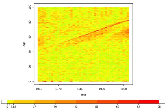
0 20 40 60 80 100 Poisson LC Year Age 1961 1970 1980 1990 2000 0 3.84 17 30 43 56 69 82 95
Figure 1: Heat map of r2xt for the PLC model, accompanied by the corresponding colour code.
Green/yellow rectangular cells indicate areas with good fit, while orage/red coloured cells indi-cate areas with significantly poor fit.
where dxt is the observed number of deaths at age x in year t and ˆµxt = exp( ˆαx+ ˆβxˆκt) is
the maximum likelihood estimate (MLE) of the underlying mortality rate. A colour-coded heat
map ofr2xtcan then be constructed to visualise the lack of fit of the PLC model to our mortality
data, as depicted in Figure 1.
Under the null hypothesis that the PLC model is the true underlying model (and some
mild conditions), eachr2xthas an approximate chi-squared distribution with degrees of freedom
one (χ21) asymptotically. Ideally, we should expect only around 5% of the rectangular cells
(AT ×0.05 = 210) to have poor fit (defined as rxt2 >3.84, where 3.84 is the 95th precentile of
χ21). However, it is evident from Figure 1 that the heat map is scattered with more than the
expected amount of orange/red cells (about 25%), and is especially obvious for the infants and ages above 40, suggesting model inadequancy in accounting for extra variations in the data. Additionally, we can also perform the Pearson’s chi-squared overall goodness of fit test. In
particular, the model deviance computed as the sum of rxt2 ,
r2=X x,t rxt2 =X x,t (dxt−extexp( ˆαx+ ˆβxκˆt))2 extexp( ˆαx+ ˆβxκˆt) ,
has a value of 15378.73. Again, under the null hypothesis that this model is a good fit to the
data, the r2 should follow an approximate chi-squared distribution with degrees of freedom
(df) given as df = (A−1)(T −2) = 3960 (see Renshaw and Haberman, 2005). Since the
model deviance of 15378.73 is substantially larger than the critical value of the conventional
chi-squared statistics (i.e. the 95th percentile of χ2(A−1)(T−2) is 4107.51), this clearly suggests
that the PLC model does not provide a satisfactory fit to the data. Note that the obvious red/orange diagonal lines displayed in Figure 1 correspond to possible cohort effects which we
do not attempt to address in this paper, but will do so in our future work. Setting aside the lack of fit of the PLC model as evidenced by the systematic pattern of orange/red cells in the heat map (mainly due to the uncaptured cohort effect), there is still a considerable amount of orange/red cells scattering around various regions in the heat map, particularly at older ages, indicating the presence of overdispersion.
In general, failure to account for overdispersion typically leads to under-smoothing, where the variance imposed by a model that ignores overdispersion forces the fitted values to adhere more closely to the data. Fundamentally, this is because the likelihood function of a model with smaller variance heavily penalizes fitted values that are distant from the observed values. This forces the fitted values to be undesirably close to the observed values which prevents an accurate
description of the underlying process. Ignoring overdispersion also leads to over-optimistic
forecast uncertainty because the extra source of uncertainty due to heterogeneity is effectively neglected. Appropriately accounting for overdispersion, on the other hand, provides a greater flexibility for the fitted values to adhere less to the observed data and allow for the possibility of greater smoothing, potentially resulting in an improved description of the underlying mortality trend. This prevents over-fitting and offers a better calibration of the unexplained variation, thereby producing a much more representative prediction interval for the associated mortality forecast (see Section 7.2 for more details).
3
Overdispersion Models
In this section, we present two models to account for overdispersion, both of which extend the PLC model in a rather straightforward manner. Both these models introduce a general dispersion parameter to relax the stringent assumption of a Poisson distribution.
3.1 Poisson Log-Normal Lee-Carter (PLNLC) Model
The first model we introduce is essentially a direct combination of the original LC model with its Poisson based equivalent, which we refer to as the Poisson Log-Normal LC model. In particular,
a normal perturbation term is added onto logµxt for an extra layer of variability in the model:
Dxt|µxt ind ∼ Poisson(extµxt) logµxt = αx+βxκt+νxt (3) νxt|σµ2 ind ∼ N(0, σµ2).
Here, σ2µ is regarded as the general dispersion parameter, whose role is to capture the global
level of extra variability in the data. The likelihood function now consists of two parts: i. f(d|logµ) = Y x,t exp(−extµxt)(extµxt)dxt dxt! ∝exp −X x,t extµxt ! Y x,t µdxt xt ; ii. f(logµ|α,β,κ, σ2µ) = Y x,t 1 q 2πσ2 µ exp − 1 2σ2 µ (logµxt−αx−βxκt)2 ∝ (σ2µ)−AT2 exp " − 1 2σ2 µ X x,t (logµxt−αx−βxκt)2 # ,
where α = (α1, α2, . . . , αA)>, β = (β1, β2, . . . , βA)> and κ = (κ1, κ2, . . . , κT)> are vectors of
parameters, while µ and d are matrices of the latent variables, µxt, and the observed death
data, dxt, respectively. Under this model,
E[Dxt] =Eµxt(EDxt[Dxt|µxt]) =extexp αx+βxκt+ 1 2σ 2 µ , (4) and Var[Dxt] = E[Dxt]× 1 +E[Dxt](exp(σ2µ)−1) >E[Dxt]. (5)
Hence, this model possesses a larger variance than its mean in general, with σµ2 governing
the relative excess spread, providing more flexibility in the model specification. Note that
equation (4) implies that the mean of Dxt under the PLNLC model is slightly different from
the PLC model (due to the extra term σ2µ/2). Some researchers (e.g. Dick, 2004) apply a
correction by directly subtractingσµ2/2 from the rate model in equation (3). However, we chose
to retain a similar model structure between the overdispersion models for easy interpretation and comparison, since the magnitude of the correction term is small relative to the overall
magnitude of logµxt.
3.2 Negative Binomial Lee-Carter (NBLC) Model
The second model is a classic extension of the Poisson distribution to incorporate overdispersion. Specifically, it is a gamma mixture of Poisson as follows:
Dxt|µxt ind ∼ Poisson(extµxt) logµxt = αx+βxκt+ logνxt (6) νxt|φ ind ∼ Gamma(φ, φ),
whereφis regarded as the general dispersion parameter in this case. Similarly, the expectation
and variance of this model are given by
E[Dxt] =extexp(αx+βxκt) (7) and Var[Dxt] = E[Dxt]× 1 +E[Dxt] φ >E[Dxt]. (8)
Therefore, this model possesses the same mean as the PLC model (as opposed to the PLNLC
model), while at the same time has a larger variance depending on the value ofφ. In particular,
the smaller the value of φ, the larger the variance, and hence the stronger the evidence of
overdispersion; while the larger the φ, the more this model approaches the PLC model, with
exact resemblance when φ → ∞. In other words, 1/φ represents the overall magnitude of
overdispersion in the data.
One attractive feature about this model is that the latent variables,µxt, can be conveniently
integrated out, producing its equivalent version, which we call the NBLC model. That is,
Dxt|αx, βx, κt, φ∼ Neg-Bin φ, φ extexp(αx+βxκt) +φ . (9)
The likelihood function now consists of only 1 part: f(d|α,β,κ, φ) = Y x,t ( Γ(dxt+φ) Γ(φ)Γ(dxt+ 1) extexp(αx+βxκt) extexp(αx+βxκt) +φ dxt φ extexp(αx+βxκt) +φ φ) ∝ φ AT φ [Γ(φ)]AT Y x,t Γ(dxt+φ) exp[dxt(αx+βxκt)] [extexp(αx+βxκt) +φ]dxt+φ .
The prominent advantage of the marginalisation is that we avoid the need to simulate the
high-dimensional µxt (dimension=AT=4200 in our case), at the expense of having a slightly
more complicated likelihood function. In particular, we found in our preliminary study that
the computational gain from marginalising µxt substantially outweighs the burden of dealing
with the more complicated negative binomial likelihood (by comparing the effective number of samples generated per unit time). Note that this model has already been considered by Delwarde et al. (2007), but within a classical framework. Hence, one of our contributions in this paper is to fit this model within a Bayesian paradigm for an integrated modelling procedure.
4
Advantages of Bayesian Mortality Modelling/Forecasting
The rationale for considering Bayesian methodology is it provides a natural framework in which prior knowledge can be incorporated and various sources of uncertainty (due to inherent random variation, parameter estimation, projection and model misspecification) can be coherently in-cluded to provide a more representative prediction interval. Classical LC approach often ignores uncertainty due to parameter estimation. Although it has been shown in Lee and Carter (1992) that the forecast uncertainty will dominate over parameter uncertainty in long term projection, the same is not true for short to moderate term projection. Computing parameter uncertainty within the frequentist framework typically necessitates bootstrapping (see for example Brouhns et al., 2005). In Bayesian framework, parameter uncertainty is incorporated in the form of probability distributions through prior specification for each of the unknown parameters. In addition, we also acknowledge the presence of model uncertainty by performing Bayesian model determination using posterior model probabilities, instead of assuming in advance, a single underlying model.
Moreover, a major criticism on the traditional LC approach is the potential inconsistencies that may arise due to its two-stage model fitting procedures: the parameters are first estimated using maximum likelihood approach, they are then separately fitted using the ARIMA time series model solely for the purpose of projection. Technically, the ARIMA model, being part of the model specification, should have contributed directly in the parameter estimation stage.
Bayesian modelling solves this issue by directly specifying an ARIMA prior on κt, forming a
single framework of a hierarchical model. Parameter estimation then proceeds simultaneously through the computation of joint posterior distribution. Additionally, this allows for the pos-sibility of performing smoothing over time (as mentioned in Czado et al., 2005), depending on the ARIMA model fitted. Projection of mortality then follows naturally within the Bayesian framework based on the ARIMA model chosen (see Section 5.5).
Furthermore, carefully calibrated percentiles of the posterior predictive distribution carry valuable information necessary to characterize the uncertainties we encounter during forecasting. In practice, any percentile can be used as a point estimate other than the posterior mean or median in the context of probabilistic forecasts (see for example Berger, 2013). This provides more flexibility to users who are involved in risk-controlled decision making.
4.1 Prior Distributions
In this section, we provide the prior distributions used for each parameters. Ideally, the prior dis-tributions chosen should reflect our uncertainty/prior knowledge about mortality (e.g. smooth-ness of mortality rates across age). However, we do not pursue this matter here. Rather, we specify some commonly used priors rendered sufficiently diffuse for data-dominated infer-ence. In addition, we also attempt to be indifferent in terms of prior specification under both overdispersion models to facilitate model comparison later on. Note that even though our prior specification differs considerably from that of Czado et al. (2005), this difference should not be consequential in terms of the parameter estimation, given the size of our mortality data.
4.1.1 Prior Distribution for αx, βx, σ2β, σµ2, andφ
From here on, we denote1n as a length−nvector of ones, while Jnand Inas a matrix of ones
and the identity matrix respectively of dimension n×n. For simplicity, we assign independent
normal priors on αx, i.e.
α∼N(α01A, σα2IA).
Here, we set α0 = 0, while σα2 is chosen to be relatively large, say σα2 = 100 for a vague prior.
Similarly, we impose, a priori
β∼N(0, σβ2IA),
subject to the constraint P
xβx = 1. Applying the constraint on the marginal prior of βx,
and using the conditional property of a normal distribution, we obtain the following prior for
β−1 = (β2, β3, . . . , βA)>, β−1 ∼N 1 A1A−1, σ 2 β IA−1− 1 AJA−1 .
That way, the constraint is automatically accounted for by the above prior withβ1
determinis-tically computed fromβ1 = 1−β2−. . .−βA. This corresponds to transforming the constraint
into a proper point mass prior on the unidentified β parameters, which automatically yields
proper posterior inference, as stated by Gelfand and Sahu (1999). They also note the issue of a slower rate of convegence of this constraint-handling approach (due to the correlations induced), which we propose to solve using the blocking strategy (see Section 5). Moreover, the
hierarchical variance,σ2β is now treated as a hyperparameter with the conventional prior
σ−β2 ∼Gamma(aβ, bβ),
where aβ =bβ = 0.001. The result of this is a heavier-tailed Student’s t-distribution on βx a
priori, characterizing our larger uncertainty inβx due to its more erratic behaviour as compared
toαx empirically.
As pointed out in Section 3.1 and 3.2, σ2µ and φ serve as the dispersion parameter in each
model. Since we have no knowledge on the appropriate extent of overdispersion in our data, we assign the conditional conjugate (see Gelman, 2006) prior
σ−µ2 ∼Gamma(aµ, bµ),
withaµ=bµ= 0.0001 for computational purposes under the PLNLC model. In order to specify
a prior with similar amount of information embedded within the distribution for φ, we need
approximation to logµxt under the NBLC model, and ignoring the variabilities due toαx,βx, and κt, we have Var(logµxt) = Var(logνxt)≈ dlogz dz 2 z=E(νxt) ×Var(νxt) = 1 φ.
Knowing that Var(logµxt) = σµ2 (conditional upon αx, βx and κt) under the PLNLC model,
this implies that a sensible prior for φcould be
φ∼Gamma(aφ, bφ),
whereaφ=bφ= 0.0001.
4.1.2 Prior Distribution for κt
For reasons mentioned in Section 4, an ARIMA time series model is imposed on κt, which can
then be straightforwardly extrapolated forward in time for mortality projection. On various
occasions, a random walk with drift was empirically found to provide an adequate fit forκt (see
Tuljapurkar et al., 2000). Following Czado et al. (2005) though, we fit a first order autoregressive (AR(1)) model with linear drift. Specifically,
κt−ηt=ρ(κt−1−ηt−1) +t, fort= 2,3, . . . , T,
κ1=η1+1,
(10)
where ηt =ψ1 +ψ2t denotes the linear drift and t
ind
∼ N(0, σ2
κ) are random errors. Note that
Equation (10) includes random walk with drift as a special case when ρ = 1, provided that
it is not ruled out a priori. In other words, we allow the data to choose either an AR(1) or random walk with drift instead of specifying beforehand the appropriate model since it is entirely possible that random walk with drift fits our data poorly. We also adopt a different constraint
forκt,κ1= 0 as compared to the conventionalPtκt= 0. This changes the interpretation ofαx
slightly, whereαxnow represents log mortality rates in the base year. Fixingκ1 = 0 also has the
effect of setting the first year as the baseline year, where values ofκtfor the remaining years are
estimated relative to the value ofκ1. In other words,κtshould be interpreted as the parameter
that represents the overall mortality trend with respect to the baseline year. Elsewhere, the
impact of this is purely computational, the posterior distribution of logµxtwill not be affected.
This model can be equivalently expressed in its multivariate form (with the constraint) as
κ−1 ∼N(Y−1ψ−ρR−1Y1ψ, σκ2Q −1) κ1= 0 , (11) where P = 0 0 · · · 0 ρ 0 ... 0 ρ . .. ... .. . . .. ... ... ... 0 · · · 0 ρ 0 (T−1)×(T−1) , Y−1= 1 2 1 3 .. . ... 1 T (T−1)×2 , Y1 = 1 1 0 0 .. . ... 0 0 (T−1)×2 ,
R=IT−1−P,Q=R>R,ψ = (ψ1, ψ2)>, andκ−1= (κ2, κ3, . . . , κT)>. For complete
specifi-cation of the model onκt, the unknown parametersρ,σ2κandψ are treated as hyperparameters
with the following standard vague priors:
where σ2ρ = 100, aκ = bκ = 0.001, ψ0 = (0,0)>, and Σψ =
1000 0
0 10
. These priors are chosen to be conditionally conjugate with respect to the AR(1) model, which ease the subsequent computation of the conditional posterior distributions as we shall see later in Section 5.
5
Computation
5.1 MCMC Method
The MCMC method we propose is the variable-at-a-time Metropolis-Hastings (MH) algorithm as described in O’Hagan and Forster (2004), where each component of the parameters are updated sequentially through MH algorithm in each iteration, conditional on the rest of the parameters. In the case where the conditional posterior distributions are tractable, typically where conditional conjugate priors are used, the Gibbs algorithm is undertaken (MH algorithm with acceptance probability equals to 1).
In addition, we will be adopting the idea of blocking of parameters wherever possible within our MCMC updating scheme. The motivation of considering blocking is the fact that it enables the MCMC algorithm to acknowledge the correlation structure of the parameters in order to make informed movements/jumps across the parameter spaces, facilitating the exploration of posterior distributions. For instance, Roberts and Sahu (1997) suggest that blocking, if done efficiently, is capable of improving the convergence rate of the resulting MCMC sampler substantially. However, the efficacy of performing blocking is clearly dictated by the dimensions of parameters involved and the resulting complexity of the conditional posterior distributions of the respective blocks. Therefore, our general strategy of blocking is to allocate highly-correlated parameters in a single block such that the correlations between blocks are reduced (rather than allocating all in one block).
5.2 MCMC Scheme for the PLNLC Model
Suppose we allocate theαx,βx andκteach in one separate block, and the rest of the parameters
updated univariately. Due to the model structure, the conditional posterior distributions of all of the parameters can be conveniently recognized as standard distributions (Appendix A),
except for the logµxt. Hence, the MCMC updating scheme for the PLNLC model can be easily
implemented by iterating through a series of Gibbs steps, together with some MH steps for
the remaining logµxt. We describe in detail the MH step for the remaining logµxt in the next
subsection.
5.2.1 MH Step for logµxt
We forfeited the concept of blocking here due to the immense dimensionality involved. Instead,
each logµxtis updated univariately using random walk MH algorithm (see for example O’Hagan
and Forster, 2004). In particular, using the assumption thatDare mutually independent given
logµ, and logµare independent elementwise given (α,β−1,κ−1, σµ2), the conditional posterior
density of logµxt can be expressed as
f(logµxt|α,β−1,κ−1,d,logµ−xt, σκ2, σβ2, ρ,ψ, σ2µ)∝µ dxt xt exp −extµxt− 1 2σ2 µ (logµxt−αx−βxκt)2 ,
where µ−xt = (µ11, µ21, . . . , µx−1t, µx+1t, . . . , µAT)> is a vector of all the mortality rates
ex-cluding thextth component. Next, we propose a value at theith iteration,
where logµixt−1is the current value of logµxt, andσ2µxt are the proposal variances to be specified
deterministically. The proposal is then accepted according to the following probability, a(logµ∗xt|logµixt−1) = min
( 1, µ∗xt µixt−1 dxt exp −ext(µ∗xt−µixt−1) − 1 2σ2 µ ((logµ∗xt−αx−βxκt)2−(logµixt−1−αx−βxκt)2) .
The choice of σ2µxt is arbitrary, but has a direct impact on the speed of convergence of the
constructed chain. In practice, σµ2xt are carefully chosen such that the acceptance rates of
logµxt are within the recommended range 0.15-0.45 (Roberts and Rosenthal, 2001). Following
Czado et al. (2005), we develop a simple automatic trial and error search algorithm for tuning
σµ2xt, which starts off with a crude search:
i. Set initial values ofσ2µxt = 0.01 for allx and t.
ii. A pilot run of 100 iterations is executed.
iii. Proposal variances that correspond to acceptance rates smaller than 0.15 are halved. iv. Proposal variances that correspond to acceptance rates exceeding 0.45 are doubled.
v. Repeat steps ii-iv until a predefined threshold is achieved (e.g. when 4000 of the acceptance rates are within 0.15-0.45).
The search can then be further refined by shrinking the increments (or decrements) of the adjustments within the above algorithm, so instead of a multiplicative factor of two, we can add (or subtract) a small amount, say 0.001, during the tuning of the proposal variances. As a
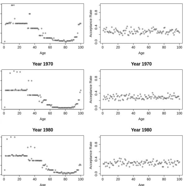
result, theσ2µxt can be numerically determined and are depicted in Figure 2.
Interestingly, σµ2xt exhibit a consistent age pattern across the years. It turns out that the
rough pattern of posterior variances of logµxt in a given year can potentially be deduced from
this set of approximate optimal proposal variances, which can be verified by referring to Ap-pendix C. This can be attributed to the finding in Roberts and Rosenthal (2001) that the optimal proposal variance for a MH algorithm with a univariate normal distribution as its
target is proportional to the posterior variance (with 2.382 as the proportionality constant).
5.3 MCMC Scheme for the NBLC Model
Here, we apply the random walk MH algorithm onα,β−1 and κ−1 instead because the normal
priors are no longer conditionally conjugate. Nevertheless, the Gibbs steps for ρ, σ2κ, σβ2,ψ are
unaffected (refer to Appendix A) because they belong to the lower part of the hierarchical model,
hence their conditional posterior distributions remain the same conditional upon α,β−1, and
κ−1. Note that our preliminary study also revealed that performing the sequential updating
scheme univariately without blocking is more efficient here in terms of the effective number of posterior samples generated per unit time.
5.3.1 MH Steps for αx, βx, κt, and φ
The conditional posterior densities and expressions for the MH acceptance probabilities are displayed in Appendix B. Using obvious notation, a set of numerically determined proposal variances for the random walk MH algorithm (derived from similar search algorithm as in
● ●●●●● ●●● ●● ● ● ● ●●●●●●●●●●●●●●●● ●● ●● ●●●●●●●●●●● ●●● ● ● ● ●● ● ●●●●●●●●● ● ● ●●●●●●●●●●●●●●●●●●●●●●●●●● ●●●● ● ●●●● 0 20 40 60 80 100 0.00 0.02 0.04 Year 1961 Age Proposal V ar iance ● ● ● ● ● ●●●●●● ● ●● ● ● ● ● ●●● ● ● ●● ● ●● ● ● ●● ●● ● ● ● ● ●● ● ● ● ●●● ● ● ●●● ● ● ● ● ●●● ● ● ● ●● ● ● ● ●●●● ● ● ●●●● ●● ● ●● ●●●●● ●●●●● ● ● ● ●● ●●● ● 0 20 40 60 80 100 0.0 0.4 0.8 Year 1961 Age Acceptance Rate ● ●●●●●● ● ●●●● ● ●●● ● ●●● ● ●●●●●●●●● ● ● ●●● ● ●●●●●●●●● ● ● ● ●●● ●●●● ●●●●●●● ●●●●●●●●●●●●●●●●●●●●●●●●●●●●●● ●●●● ●● ● ● 0 20 40 60 80 100 0.01 0.03 Year 1970 Age Proposal V ar iance ● ● ● ● ● ● ● ● ● ● ●● ● ● ● ●● ● ●● ● ● ● ●● ●● ●●●● ●● ●● ●●●● ● ● ● ● ●● ● ●● ● ● ●●●● ● ●● ●● ● ●● ●● ● ● ● ● ● ●●● ● ●● ● ●● ●●●●●● ● ●● ● ● ● ● ● ● ● ●●●●● ● 0 20 40 60 80 100 0.0 0.4 0.8 Year 1970 Age Acceptance Rate ● ●● ● ●●●● ● ●●●● ● ●●●●●●●●●●●●●●●● ● ●●● ● ● ●●● ● ●●●●●●●●● ● ●●●● ● ● ●●●●●●●● ●● ● ●●●●●●●●● ●●●●●●●●●●●●●●● ●●● ●●● ●●● 0 20 40 60 80 100 0.00 0.02 0.04 Year 1980 Age Proposal V ar iance ●●● ● ● ● ●● ● ● ●● ●● ● ● ●●●● ● ● ● ● ● ● ●● ● ● ● ●● ● ● ●●●● ● ●●● ● ● ● ●● ● ●● ● ● ● ●● ●● ●● ● ●● ● ● ● ● ●● ●● ●●●●●● ●● ● ●● ●● ● ● ● ● ● ●● ● ●● ●● ●● ●● 0 20 40 60 80 100 0.0 0.4 0.8 Year 1980 Age Acceptance Rate
Figure 2: Plots of proposal variances,σ2µxt (left panels) and the corresponding acceptance rates
of µxt (right panels) for years 1961, 1970 and 1980 under the PLNLC model.
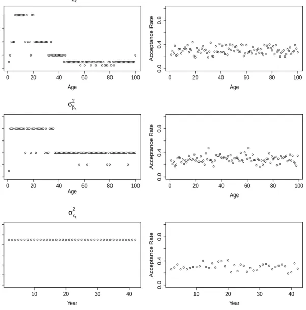
According to Figure 3, σ2
αx demonstrates a rather similar age pattern to σ
2
µxt at any given
time as before. This is perhaps not so surprising since αx represent the log mortality rates in
the base year. However, the age pattern exhibited by σ2β
x is less sensitive to age than those
of the σ2
µxt as well asσ
2
αx, albeit still having a rather similar pattern. On the other hand, the
σκ2t derived from the search algorithm, are strikingly identical across the years. This signifies
that the marginal posterior variances of κt are very similar, in contrast to αx and βx, where
their proposal variances vary substantially across ages. To verify that the marginal posterior variances of these parameters do exhibit similar shapes as the chosen proposal variances, please refer to Appendix C.
A proposal variance of σ2
φ = 0.08 will return an acceptance rate of approximately 0.30 for
● ● ●●● ●●●●●●●● ● ● ●● ● ●● ●●●●●●●●●●● ●● ● ●●●●●●●●● ● ● ●●●●●●●●●●● ● ●● ● ●●●● ● ●●● ● ●●●● ● ● ●●● ●● ● ● ● ●●●●●●●●●●●●●●●● ● 0 20 40 60 80 100 0.000 0.004 0.008 σα2x Age Proposal V ar iance ● ● ● ● ●● ●● ●● ●●● ● ●●● ● ●● ● ●●● ●● ●● ● ● ● ● ●● ● ● ●● ● ● ● ● ● ● ● ● ● ● ● ● ●● ●●● ●● ●● ● ●●●● ● ● ● ●● ● ● ● ● ● ● ● ● ● ● ● ● ● ● ●● ● ●●● ●● ● ● ● ●● ● ● ● ● 0 20 40 60 80 100 0.0 0.4 0.8 Age Acceptance Rate ● ●●● ● ●●●●●●●● ● ●●● ● ●●● ● ●●●●●● ● ● ●● ●●●● ●●●●●●●●●●●●●●●●●●● ● ●●●●● ● ●●●●●●●●●●●●●●● ● ● ● ●●●●●●●●●●●●● ● ●●●●●● 0 20 40 60 80 100 0 2 4 6 8 10 σβ2x Age Proposal V ar iance ( 1 × 10 − 7) ● ●● ●● ●●● ● ● ● ● ●● ● ●●● ● ●●●● ● ●● ● ● ● ● ●● ● ● ● ●●●● ●●●●●● ● ● ● ● ●●●● ● ● ●● ● ● ● ● ● ● ● ●● ● ●● ● ● ● ●●●● ● ● ● ●●● ● ● ● ● ●●●● ●● ● ● ● ● ● ● ● 0 20 40 60 80 100 0.0 0.4 0.8 Age Acceptance Rate ● ● ● ● ● ● ● ● ● ● ● ● ● ● ● ● ● ● ● ● ● ● ● ● ● ● ● ● ● ● ● ● ● ● ● ● ● ● ● ● ● 10 20 30 40 0 1 2 3 4 5 6 σκ2t Year Proposal V ar iance ●● ● ●●●●● ● ● ● ●● ● ● ● ● ● ● ● ● ● ●● ● ● ● ● ●● ●● ●● ●●● ●● ● ● 10 20 30 40 0.0 0.4 0.8 Year Acceptance Rate
Figure 3: Plots of the proposal variances (top panels), σ2αx, σβ2x, σκ2t, and their corresponding
acceptance rates (bottom panels) for the NBLC model.
5.4 Generating µxt under the NBLC Model
Although the mortality rates, µxt, have been integrated out for the NBLC model, it can still
be useful to simulate them to potentially learn about their posterior distributions. The latent
variables can be retrieved by noting that for anyx= 1, . . . , Aand t= 1, . . . , T,
f(µxt|d) = Z
f(µxt|αx, βx, κt, φ,d)f(αx, βx, κt, φ|d)dαxdβxdκtdφ,
wheref(αx, βx, κt, φ|d) is the joint posterior density ofαx,βx,κt, andφ, whilef(µxt|αx, βx, κt, φ,d)
can be derived as f(µxt|αx, βx, κt, φ,d)∝µ(dxt+φ) −1 xt exp − ext+ φ exp(αx+βxκt) µxt ,
implying that µxt|αx, βx, κt, φ,d∼Gamma dxt+φ, ext+ φ exp(αx+βxκt) . (12)
Therefore, the posterior samples ofµxt can be generated by simulating from the expression in
(12), where the joint posterior samples of αx, βx, κt, and φ (which are readily available from
our MCMC outputs) are substituted wherever applicable.
5.5 Mortality Forecast
Projection within the Bayesian framework is particularly natural through the derivation of posterior predictive distribution. Specifically, the posterior predictive distribution of 1-year ahead log mortality rates for each age group (with the age parameters held fixed), under the PLNLC model for instance, can be written as
f(logµx T+1|d) = Z
f(logµx T+1|αx, βx, κT+1, σµ2)f(αx, βx, σ2µ|d)f(κT+1|κT, ρ, σ2κ,ψ) ×f(κT, ρ, σ2κ,ψ|d)dαxdβxdκTdκT+1dρdσ2κdψdσµ2, (13)
wheref(αx, βx, σµ2|d) andf(κT, ρ, σκ2,ψ|d) are the joint posterior distributions. Hence, posterior
uncertainties, with respect to the model likelihood, prior distributions and the projection model, are fully integrated in the posterior predictive distribution. The density in (13) is analytically intractable, but can be empirically estimated using our MCMC samples. Essentially, generation
of the posterior samples of logµx T+1 proceeds in two steps:
1. GenerateκT+1 from the AR(1) model,
κT+1 ∼N(ψ1+ψ2(T + 1) +ρ(κT −ψ1−ψ2T), σκ2),
where joint posterior samples of (κT, ρ, σκ2, ψ1, ψ2) from the MCMC output are substituted
into the expression.
2. Generate logµx T+1 from
logµx T+1 ∼N(αx+βxκT+1, σµ2),
where κT+1 is from step 1 and (αx, βx, σ2µ) are joint posterior samples from the MCMC
output.
By analogy,h-year ahead projections can be obtained by recursive implementation of the above
generation procedures. Having generated a set of posterior predictive samples, a fanplot of carefully calibrated percentiles (see Abel, 2015) can then be constructed to better visualise the underlying uncertainty associated with our probabilistic forecast.
Once the future underlying mortality rates, for instance logµx T+h , have been simulated,
we can generate the h-year ahead number of deaths simply through
Dx T+h ∼Poisson(ex T+hµx T+h),
where ex T+h is the future exposure at age x in year T +h (which we assumed known). The
future crude mortality rates can subsequently be obtained by ˆ
µx T+h=
Dx T+h
ex T+h
The key difference between them is that the projected crude mortality rates include the Poisson variation in their prediction intervals, whereas the projected underlying mortality rates do not. The choice of which one to use depends on the users’ preference, whether or not they prefer to base their policy making on the underlying rates (unobservable), or the crude rates (observable). We chose to present the projected crude mortality rates in the result section purely because plots of observable quantities provide a more sensible visualisation in terms of validating the models against the observed crude death rates (see Section 7.3). Indeed, it should also be noted that computation of the future crude death rates requires the availability of future exposures, which can be an unrealistic assumption at times.
6
Initialization and Convergence Diagnostics
For initialization ofα,β−1 and κ−1, we use the MLEs obtained using Goodman’s method (see
Renshaw and Haberman, 2005). On the other hand, the initial values ofσκ2 andρ are obtained
by fitting an AR(1) with linear drift model onκ(using the ‘arima’ function within the ‘forecast’
package in R), whileσ2β is initialised by the empirical variance of the MLEs of β. Finally,ψ is
initialised as (0,0)>, while the overdispersion parameters, σµ2 andφ, are initialised by 0.01 and
100 respectively. Under the PLNLC model, the latent parameters, µxt, are initialized using the
empirical death rates, dxt/ext. Note that the initialization is proposed based on values close
to the MLEs to possibly speed up convergence, but should not be impactful in terms of the parameter estimation. Ideally, multiple chains with different initializations should be run to ascertain the convergence of the chains. Specifically, Gelman and Rubin (1992) proposed the use of multiple sequences with starting values initialised from an overdispersed distribution, and developed a quantity as a function of within and across chains variance to assess convergence. Instead, we assume here that a burn-in phase of 10000 iterations is sufficiently long to mitigate
the effect of initialization. In addition, we applied 100th posterior sample thinning (collecting
one realization every 100 iterations) for each of the parameters to reduce the autocorrelations of these series. After discarding the burn-in iterations and applying thinning, we obtain a sample of size 10000 for each of the paramaters under the NBLC model and a sample of size 100000 for those under the PLNLC model (a larger sample size is required to learn about the posterior under the PLNLC model due to high-dimensionality).
Before making any inferential comparisons, trace plots and auto-correlation plots (see for example Lunn et al., 2013) can be used as diagnostic tools for detecting anomalies in the MCMC generated posterior samples. By referring to Appendix D, the trace plots of some of the randomly selected parameters emerge as if convergence has been attained, with proper mixing and no apparent anomaly. The sample auto-correlations also appear to decay fairly quickly
after applying thinning, except perhaps κt, which are relatively more correlated. In summary,
the MCMC generated posterior samples seem to be well-behaved and, thus, are ready to be used to perform subsequent computations for accurate inferences to be drawn.
7
Numerical Results
In this section, we compare our proposed models with the Bayesian PLC model (i.e. the PLNLC
model or NBLC model without the overdispersion component, νxt) by Czado et al. (2005) to
highlight the importance of accounting for overdispersion. The data used for this purpose are as described in Section 2.1. The Bayesian PLC model is fitted using Czado’s methodology, except we adopt the same prior specification as in Section 4.1 (for all the parameters and hyperparam-eters involved) to facilitate model comparison later on. We also provide a comparison of our
proposed models with each other.
7.1 Estimated Parameters
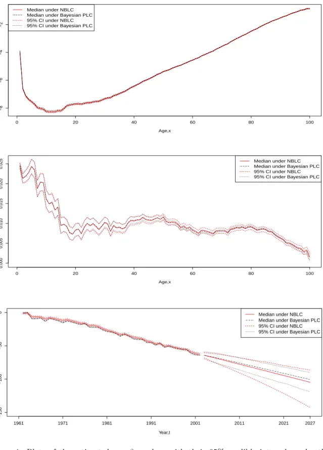
Figures 4 depicts the fitted values (posterior medians) of α, β and κ, accompanied by the
associated 95% credible intervals (computed from the sample quantiles) under the Bayesian
PLC and NBLC models. Also included is the projection of κt, 25 years into the future (until
year 2027), for illustrative purposes. Note that the fitted values under the PLNLC model are not displayed for some of the plots here because they almost coincide with those of the NBLC model, and hence are excluded for a better visualisation. According to Figure 4, the fitted
values of α and β under these models are rather similar (because the same vague priors are
specified across the models), with the overdispersion models producing slightly wider credible intervals in general. This is the general feature of a model which accounts for overdispersion,
where the responses (Dxt) are allowed to have more variabilities due to the extra flexibility
offered by the model likelihood, permitting the parameters to be more volatile, and hence, the wider credible intervals. Additionally, the width of the credible intervals also appears to be noticeably different as age increases.
The main difference arises from the parameter κ, where the fitted values are larger and
much smoother under the overdispersion models (with arguably wider credible intervals yet again). Furthermore, in terms of projection, not only do the overdispersion models forecast
a larger mortality improvement (indicated by more negative values of the projected κt), the
corresponding prediction intervals for the projected κt are also substantially wider. This is
perhaps a little interesting considering that the same AR(1) prior is imposed on κt under all
approaches. An intuitive explanation for this is that the dispersion parameter provides more flexibility for the model to describe the variabilities present in the data (where the model likelihood penalizes less on fitted values that are distant from the observed data due to the larger variance postulated), thereby allowing more priority to be put on fitting the AR(1) prior during the Bayesian estimation, hence the smoother fitted values. On the other hand, with less
variabilities imposed for Dxt under the Bayesian PLC model, their fitted values are restricted
to stay close to the observed values, implying that less smoothing is applied. The exact reason
behind this finding will be further explored when the marginal posterior distribution of ρ is
examined in the next paragraph.
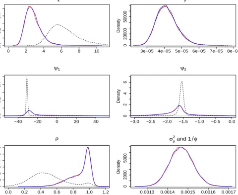
Kernel estimates of the marginal posterior density of the rest of the parameters, derived from
the posterior samples, are presented in Figure 5. The kernel densities ofσ2β are almost identical.
The most apparent discrepancies occur at the marginal posterior of σκ2 and ρ. Specifically,
the density of σ2κ for the Bayesian PLC model concentrates more at higher values, suggesting
larger residuals for κt under this model. Interestingly, the marginal posterior of ρ has the
same characteristics as a two-component mixture distribution under all models, consisting of a
stationary AR(1) component (ρ <1) and a non-stationary component close to a random walk
(ρ = 1). Closer inspection shows that peaks of the marginal posterior of ρ occur at 0.42 and
1 for Bayesian PLC model, while for the overdispersion models, the peaks are at 0.85 and 1.
This indicates that the projection model fitted on κt, in some sense, resembles a mixture of a
stationary AR(1) model and a random walk with drift model. In addition, the allocation of proportion is also different, with the overdispersion models allocating a higher proportion for
the peak at around ρ= 1 than the Bayesian PLC model.
The marginal posterior of ρ enables us to justify our earlier findings onκt. Firstly, as the
fitted ρ increases towards larger values for the overdispersion models, the fitted time series
model imposes a stronger smoothing on κt. Hence, the smoother fitted κt for this model as
0 20 40 60 80 100 −8 −6 −4 −2 Age,x αx Median under NBLC Median under Bayesian PLC 95% CI under NBLC 95% CI under Bayesian PLC 0 20 40 60 80 100 0.000 0.005 0.010 0.015 0.020 0.025 Age,x βx Median under NBLC Median under Bayesian PLC 95% CI under NBLC 95% CI under Bayesian PLC −150 −100 −50 0 Year,t κt 1961 1971 1981 1991 2001 2011 2021 2027 Median under NBLC Median under Bayesian PLC 95% CI under NBLC 95% CI under Bayesian PLC
Figure 4: Plots of the estimated αx, βx and κt with their 95% credible intervals under the
Bayesian PLC model and the NBLC model. The 25-years ahead projection of κt, accompanied
these models because their projection model is largely dominated by the values of ρ ≈ 1 that
almost correspond to a random walk model (ρ = 1), and a random walk model is known to
produce relatively wider intervals than a stationary AR(1) model. Note also that this effect
overshadows the fact that the residual variance, σκ2, is larger for the Bayesian PLC model.
Nevertheless, the projections of κt into the future under these models are expected to exhibit
less explosive behaviour than what would be obtained if a pure random walk with drift was used.
There are also slight differences forψ1 andψ2 between the models, with the overdispersion
models yielding heavier tails in both cases. Fundamentally, this is directly related to the mixture
posterior distribution of ρ, where when a random walk model (ρ= 1) is used, the model on κt
reduces to
κt=κt−1+ψ2+t,
whereψ2 is now the drift term, andψ1 becomes a redundant parameter that is non-identifiable
under the model, hence, the large uncertainty. To be more specific, the conditional posterior
distribution of ψ1 reduces analytically to N(0,1000) when ρ = 1, which does not depend on
the data and other parameters. This implies that its marginal posterior distribution is indeed
N(0,1000), which is exactly the same as its prior distribution. This happens because ψ1 and
ψ2 are assumed to be independent a priori, so nothing is learned about ψ1 given that it is a
non-identifiable parameter as far as the likelihood is concerned. In other words, the posterior
distribution of ψ1 also behaves like a mixture distribution, formed by mixing its prior
distri-bution (which is relatively vague) and the posterior distridistri-bution when ρ < 1. On the other
hand, all the uncertainties regarding the drift ofκtare now absorbed by ψ2 since it is the only
remaining drift parameter whenρis very close to 1, hence a heavier tail for the marginal
poste-rior distribution of ψ2. Therefore, with the overdispersion models highly favouring values ofρ
that are close to 1 (corresponding to a random walk model), the much heavier-tailed posterior
distributions for ψ1 and ψ2 are justified.
Regarding the overdispersion parameters, there is a substantial amount of Bayesian learning
for both σµ2 and 1/φ, as indicated by the obvious shifts of their posterior distributions (proper
unimodal distributions with 95% quantiles of around [0.00136,0.00158]) from the arbitrarily
dif-fuse prior distributions (which have close to negligible densities for the region of values presented in Figure 5). Recall also that the Poisson distribution is the limiting case of a negative binomial
distribution as φ→ ∞ (or 1/φ→ 0). Based on the MCMC samples generated, the posterior
median ofφis approximately 681 (1/φ= 0.001468), implying that the level of overdispersion is
non-negligible. To further strengthen this argument, we can assess the practical significance of
the magnitude of this value ofφestimated using the expression for the variance ofDxtunder the
NBLC model, given in Equation (8). The term E[Dxt]
φ can be interpreted as the relative increase
in the variance of Dxt with respect to its mean, which measures the extent of overdispersion
in the mortality data. For the purpose of a simple illustration of the level of overdispersion
implied, a crude calculation can be carried out by replacing E[Dxt] with observed deaths. For
example, using the mean observed number of deaths and the median ofφ, we obtain a value of
2846.945/681≈ 4,implying that there is a roughly four times increase in the variance of Dxt
(relative to the mean) on average under the NBLC model. More importantly, for the age and
time with the largest observed number of deaths, the relative increase is 12399/681≈18,which
is massive. Both these examples indicate that the extent of overdispersion implied by the value
of φfitted is rather substantial, and hence, should not be ignored. On the other hand, for the
PLNLC model, the Bayesian PLC model can be retrieved whenσµ2 = 0. Since the posterior
me-dian ofσ2µis around 0.001465, this indicates again the presence of non-negligible overdispersion.
Similar calculation as above can be undertaken for an interpretation of the magnitude of the
0 2 4 6 8 10 0.0 0.2 0.4 σk2 Density
3e−05 4e−05 5e−05 6e−05 7e−05 8e−05
0 20000 50000 σβ2 Density −40 −20 0 20 40 0.0 0.2 0.4 ψ1 Density −3.0 −2.5 −2.0 −1.5 −1.0 −0.5 0.0 0 2 4 6 ψ2 Density 0.0 0.2 0.4 0.6 0.8 1.0 1.2 0 1 2 3 4 5 6 ρ Density 0.0013 0.0014 0.0015 0.0016 0.0017 0 2000 5000 σµ2 and 1 φ Density
Figure 5: Kernel density plots of σκ2, σ2β, ψ1, ψ2, ρ, and φ under the Bayesian PLC (black
dotted), PLNLC (blue solid) and NBLC model (red solid).
in the variance of Dxt over its mean. It is straightforward to see that the variance ofDxt can
easily increase by several folds for this value of σ2µ(= 0.001465). For instance, replacingE[Dxt]
with max [dxt] = 12399 yields a relative increase of 12399×(exp(0.001465)−1)≈18, suggesting
the practical significance of accounting for overdispersion.
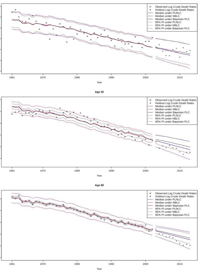
7.2 Fitted Crude Mortality Rates
Figure 6 shows the fitted and projected log mortality rates for ages 30, 55 and 80 plotted against time, 11 years into the future. According to the figure, there are considerable differences between the Bayesian PLC model and the overdispersion models in terms of the fitted rates. Firstly, the median fitted rates for the overdispersion models are slightly smoother than the Bayesian PLC model across the ages. More crucially, the credible intervals of fitted rates for the overdispersion models are substantially wider than that of the Bayesian PLC model. These are consistent with our conjecture before on the failure to account for overdispersion, where the fitted values are generally under-smoothed due to the model’s rigid structure as evidenced by the zig-zag patterns of the medians and are accompanied by over-optimistic credible intervals due to the lower variance by construction. In other words, we witness here that ignoring overdispersion has the tendency to force the fitted values to adhere more closely to the data due to the smaller variance imposed by the model (over-fitting), causing under-smoothing and narrower intervals. Both of these properties, when projected into the future, are detrimental to the resulting mortality forecasts due to the poor description of underlying trends and variabilities. On the contrary, the greater flexibility of the overdispersion models allow the fitted values to adhere less to the data (encouraging more smoothing), where the residuals due to the unexplained variations are then absorbed into the dispersion parameters, resulting in wider intervals in general. The trade-off
between adherence to the data and smoothness clearly favours the overdispersion models here, where their credible intervals provide reasonably good coverages of the observed rates across the ages, with most points lying within the intervals, while the credible intervals for the Bayesian PLC model appear to be overly narrow, with a large number of points still lying outside the intervals (particularly for age 55).
7.3 Projected Crude Mortality Rates and Out-of-Sample Validation
According to Figure 6, the overdispersion models clearly forecast a larger improvement in the mortality rates, and also produce considerably wider prediction intervals in all cases (and for the rest of the ages). This is a sensible result as Lee and Miller (2001) illustrated that the original LC approach has a tendency to underestimate mortality improvement, which may well be inherited by the Bayesian PLC model. Moreover, the prediction intervals under the Bayesian PLC model also appear to be implausibly narrow, which is consistent with the findings by Alho (1992). This
can also be explained by the time series model fitted on κt, where the overdispersion models
favour a random walk with drift model (which is known to produce wide prediction intervals). Hence, the inclusion of dispersion parameters provides a more sensible improvement in the rates as well as better calibrated probabilistic intervals in terms of the projection.
Then, we validate the candidate models against the holdout data to assess their predictive abilities. First, this is undertaken based on a disaggregate mortality quantity, the projected age-specific crude mortality rates as shown in Figure 6, derived using the projected underlying mortality rates and the holdout exposure data (see Section 5.5). The performances of the models in terms of their coverages vary across ages. In particular, the median projections of mortality improvement and the associated 95% prediction intervals for age 30 are rather similar across all three candidate models, with good predictive properties (appropriately projected past trend with good coverages for the prediction intervals) when assessed against the holdout samples. On the contrary, the projected mortality improvements for age 55 are somewhat pessimistic,
especially for the Bayesian PLC model. In particular, the coverage of the 95% prediction
intervals for the Bayesian PLC model is rather low due to the overly narrow intervals, while the overdispersion models yield prediction intervals that are wide enough to cover most of the holdout rates. For age 80 (where it is rich in death data), the coverages of all of the models are satisfactory, with the overdispersion models slightly outperforming the Bayesian PLC model by having smaller biases and better coverages. Overall, the validation process using the disaggregate mortality quantity indicates that the overdispersion models outperform the Bayesian PLC model in terms of predictive ability for this particular dataset.
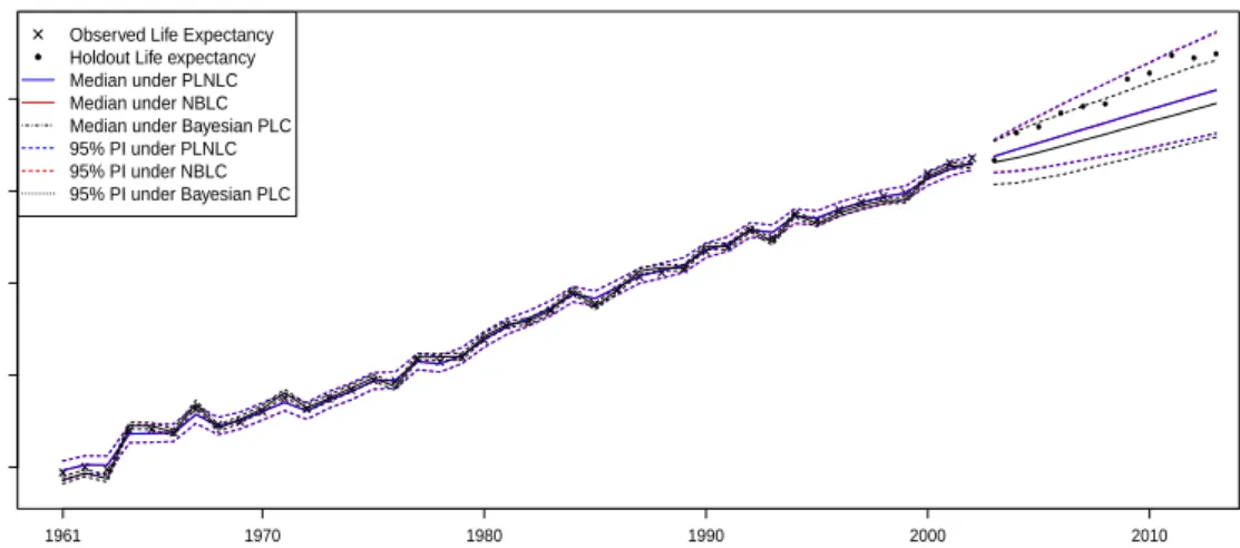
It is perhaps more useful to perform the validation based on an aggregate mortality quantity (instead of focusing on a specific age), the life expectancy at birth, derived from the projected crude mortality rates (where the holdout central exposed to risks are used). As illustrated in Figure 7, the overdispersion models forecast larger life expectancies at birth consistently and produce wider prediction intervals than the Bayesian PLC model. Moreover, the holdout life expectancies at birth all lie well within the 95% prediction intervals of the overdispersion models, while the Bayesian PLC model clearly underestimates the gains in the future life expectancy at birth, as well as producing an overly narrow prediction interval. All in all, the overdispersion models offer a better predictive power than their counterpart for this particular dataset. One concern is that the overdispersion models seemingly also yield a systematic underestimation of the life expectancy, even though their prediction intervals provide satisfactory coverages.
−8.2 −8.0 −7.8 −7.6 −7.4 −7.2 −7.0 Age 30 Year 1961 1970 1980 1990 2000 2010 ●
Observed Log Crude Death Rates Holdout Log Crude Death Rates Median under PLNLC Median under NBLC Median under Bayesian PLC 95% PI under PLNLC 95% PI under NBLC 95% PI under Bayesian PLC ● ● ● ● ● ● ● ● ● ● ● −5.8 −5.6 −5.4 −5.2 −5.0 −4.8 Age 55 Year 1961 1970 1980 1990 2000 2010 ●
Observed Log Crude Death Rates Holdout Log Crude Death Rates Median under PLNLC Median under NBLC Median under Bayesian PLC 95% PI under PLNLC 95% PI under NBLC 95% PI under Bayesian PLC ● ● ● ● ● ● ● ● ● ● ● −3.4 −3.2 −3.0 −2.8 −2.6 −2.4 Age 80 Year 1961 1970 1980 1990 2000 2010 ●
Observed Log Crude Death Rates Holdout Log Crude Death Rates Median under PLNLC Median under NBLC Median under Bayesian PLC 95% PI under PLNLC 95% PI under NBLC 95% PI under Bayesian PLC ● ● ● ● ● ● ● ● ● ● ●
Figure 6: Plots of the observed log crude death rates, log(dxt/ext), fitted log crude death rates
and the associated 11-years ahead projection of the crude log death rates for age 30 (upper panel), age 55 (middle panel) and 80 (lower panel) under the Bayesian PLC model and the overdispersion models, accompanied by 95% credible intervals.
74 76 78 80 82 Years Lif e Expectancy at Bir th 1961 1970 1980 1990 2000 2010 ● ● ● ● ● ● ● ● ● ● ● ●
Observed Life Expectancy Holdout Life expectancy Median under PLNLC Median under NBLC Median under Bayesian PLC 95% PI under PLNLC 95% PI under NBLC 95% PI under Bayesian PLC
Figure 7: Plots of the observed, fitted life expectancy at birth and the associated 11-years ahead forecast under the Bayesian PLC and the overdispersion models, accompanied by the 95% prediction intervals.
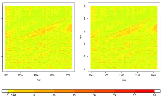
7.4 Model Assessment
We can similarly construct a heat map of the squared Pearson residuals for the overdispersion models. Expressions of the squared Pearson residuals for the PLNLC and NBLC models are given respectively as
[dxt−extexp(αx+βxκt+σ2µ/2)]2
extexp(αx+βxκt+σµ2/2) +e2xt[exp(σµ2)−1] exp(2(αx+βxκt) +σµ2)
, and [dxt−extexp(αx+βxκt)]2 extexp(αx+βxκt) h 1 +extexp(αx+φβxκt) i,
where now the posterior mean of the parametersαx,βx,κt,σ2µ and φare substituted into the
expression for an estimate. As illustrated in Figure 8, the heat maps of the overdispersion models are much “greener” than before (Figure 1), indicating an overall improvement in goodness of fit.
The sum of squared Pearson residuals for the PLNLC and the NBLC model are now 4235.24 and
4235.83 respectively, which are considerably smaller than 15378.73 of the original PLC model,
and 15379.91 of the Bayesian PLC model. The improvement is substantial, but is still not ideal
mostly because of the un-captured cohort effects, emerged as yellow/orange diagonal lines in Figure 8. Nevertheless, it is rather obvious that the overdispersion models outperformed both the original PLC and Bayesian PLC model by a considerable margin.
Note that the distribution of the sum of squared Pearson residuals, is no longer Chi-squared, but can be properly calibrated against its empirical distribution to then carry out posterior predictive checking. Following Gelman et al. (1995), we first generate a set of replicated data,
drep, which has a density representation
fM(drep) = Z
0 20 40 60 80 100 NBLC Year Age 1961 1970 1980 1990 2000 0 20 40 60 80 100 PLNLC Year Age 1961 1970 1980 1990 2000 0 3.84 17 30 43 56 69 82 95
Figure 8: Heat map of squared Pearson residuals,rxt2 , under the PLNLC model (left panel) and
the NBLC model (right panel), accompanied by the corresponding colour code.
from the posterior samples ofθM under each model, whereMis the model indicator,fM(drep|θM)
is the likelihood function, fM(θM|d) is the posterior of θM. Next, we define our test quantity
as T(d,θM) = X x,t (dxt−E[Dxt|θM, M])2 Var[Dxt|θM, M] ,
which is the usual χ2 discrepancy (that depends on both the data and parameters). An
ex-pression of T(d,θM) for each of the models under consideration is presented in Appendix E.
The test quantity is then evaluated at the replicated data to yield T(drep,θM), from which
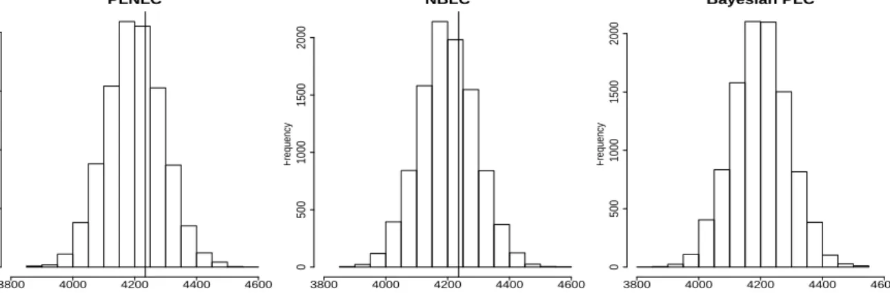
histograms can be constructed (Figure 9). The sum of squared Pearson residuals (or
equiva-lently T(d,θ¯M), where ¯θM is the posterior mean under model M) for each model is displayed
in Figure 9 to highlight the magnitude of its discrepancy with the T(drep,θM). It can be seen
that the sum of squared Pearson residuals for the overdispersion models lies somewhere in the
middle of the histograms; while that of the Bayesian PLC model (15379.91) is completely off
the charts. Moreover, the posterior predictive p-value, defined as
pB= Pr(T(drep,θM)≥T(d,θM)|d),
can be used to assess statistical significance formally. In practice, it is easily computed as the
proportion of the predictive test quantity,T(drep,θM), which equals or exceeds the realized test
quantity,T(d,θM). The posterior predictive p-values of the PLNLC, NBLC and Bayesian PLC
models are 0.0161, 0.0156 and 0.00 respectively. Therefore, there is no evidence at 1% level that
the overdispersion models are inadequate in this aspect of the data; while the extreme p-value of the Bayesian PLC model strongly indicate model inadequacy.
PLNLC Frequency 0 500 1000 1500 2000 3800 4000 4200 4400 4600 NBLC Frequency 0 500 1000 1500 2000 3800 4000 4200 4400 4600 Bayesian PLC Frequency 0 500 1000 1500 2000 3800 4000 4200 4400 4600
Figure 9: Histograms of T(drep,θM) for the PLNLC, NBLC, and Bayesian PLC model, with
their corresponding sum of squared Pearson residuals,r2 included as the vertical solid lines.
7.5 Bayesian Model Determination
Most of the previous results suggest that the two overdispersion models are very similar. This prompts the initiative to compare the fitted log mortality rates using sample quantiles-quantiles (QQ) plots. It is evident from Appendix F (Figure F.1) that all of the sample QQ plots appear to lie reasonably close to the reference line, with no peculiar behaviour (no U or S-shape). This
suggests that the posterior distributions of logµxt have similar skewness and tail distributions
under both overdispersion models. Furthermore, the QQ plot of σµ2 against 1/φ is remarkably
close to the reference line as depicted in Appendix F (Figure F.2), suggesting that their posterior distributions are essentially the same. In other words, the overall level of overdispersion indi-cated under both models are virtually the same, supporting our conjecture derived from Taylor’s approximation (Section 4.1). Again, this signifies model similarity. Therefore, Bayesian model comparison is carried out to ascertain this observation.
Formal Bayesian model comparison proceeds through the computation of posterior model
probabilities (e.g. Kass and Raftery, 1995). For a set of modelsM ∈MS under consideration,
the posterior model probability of model M,f(M|d) is given by
f(M|d) = Pf(M)fM(d) j∈MSf(j)fj(d)
,
where fM(d) is the marginal likelihood (ML) of model M and f(M) is the prior model
prob-ability of model M. Typically, we assume equal prior model probabilities so that models are
compared directly using their MLs, expressed as fM(d) =
Z
fM(d|θM)fM(θM)dθM, (14)
which is effectively the normalising constant of the joint posterior distribution. For the compu-tation of MLs, we use bridge sampling (Meng and Wong, 1996), which is an efficient method of approximating ratio of normalising constants. In the context of approximating ML, we con-struct the bridge sampling algorithm such that the second normalising constant is known. In particular, the asymptotically optimal iterative formula for bridge sampling suggested by Meng