lavaan : An R Package for Structural Equation Modeling

(1)

May 2012, Volume 48, Issue 2. http://www.jstatsoft.org/

lavaan: An

R

Package for Structural Equation

Modeling

Yves Rosseel Ghent University

Abstract

Structural equation modeling (SEM) is a vast field and widely used by many applied researchers in the social and behavioral sciences. Over the years, many software pack-ages for structural equation modeling have been developed, both free and commercial. However, perhaps the best state-of-the-art software packages in this field are still closed-source and/or commercial. The Rpackagelavaanhas been developed to provide applied researchers, teachers, and statisticians, a free, fully open-source, but commercial-quality package for latent variable modeling. This paper explains the aims behind the develop-ment of the package, gives an overview of its most important features, and provides some examples to illustrate howlavaanworks in practice.

Keywords: structural equation modeling, latent variables, path analysis, factor analysis.

1. Introduction

This paper describes packagelavaan, a package for structural equation modeling implemented in theRsystem for statistical computing (RDevelopment Core Team 2012). The package is available from the ComprehensiveRArchive Network (CRAN) at http://CRAN.R-project. org/package=lavaan and supported by the website http://lavaan.org/. lavaan is an acronym for latent variable analysis, and its name reveals the long-term goal: to provide a collection of tools that can be used to explore, estimate, and understand a wide family of latent variable models, including factor analysis, structural equation, longitudinal, multilevel, latent class, item response, and missing data models (Skrondal and Rabe-Hesketh 2004;Lee 2007;Muth´en 2002).

However, the development of lavaan has only begun and much remains to be done to reach this ambitious goal. To date, the development of lavaanhas focused on structural equation modeling (SEM) with continuous observed variables (Bollen 1989), which is the focus of this

(2)

paper. Structural equation models encompass a wide range of multivariate statistical tech-niques. The history of the field traces back to three different traditions: (1) path analysis, originally developed by the geneticist Sewall Wright (Wright 1921), later picked up in sociol-ogy (Duncan 1966), (2) simultaneous-equation models, as developed in economics (Haavelmo 1943; Koopmans 1945), and (3) factor analysis from psychology (Spearman 1904; Lawley 1940; Anderson and Rubin 1956). The three traditions were ultimately merged in the early 1970s and although many different researchers have made significant contributions (Jöreskog 1970; Hauser and Goldberger 1971;Zellner 1970; Keesling 1973; Wiley 1973; Browne 1974), it was the work of Karl Jöreskog (Jöreskog 1973), that came to dominate the field. Not least because he (together with Dag Sörbom) developed a computer program called LISREL (for LInear Structural RELations), providing many applied researchers access to this new and exciting field of structural equation modeling. From 1974 onwards, LISREL was distributed commercially by Scientific Software International. In the following decades, the wide avail-ability ofLISREL initiated a methodological revolution in the social and behavioral sciences. Today, almost four decades later, LISREL 8 (Jöreskog and Sörbom 1997) is still one of the most widely used software packages for structural equation modeling.

In the years after the birth of LISREL, many technical advances were made and several new software packages for structural equation modeling were developed. Some of the more popular ones that are still in wide use today are EQS (Bentler 2004), AMOS (Arbuckle 2011) and Mplus (Muth´en and Muth´en 2010), all of which are commercial. The few non-commercial SEM programs outside theRenvironment areMx (Neale, Boker, Xie, and Maes 2003) (free, but closed-source), andgllamm, which is implemented inStata(Rabe-Hesketh, Skrondal, and Pickles 2004).

Within theRenvironment, there are two approaches to estimate structural equation models. The first approach is to connect R with external commercial SEM programs. This is often useful in simulation studies where fitting a model with SEM software is one part of the simulation pipeline (see, for example, van de Schoot, Hoijtink, and Dekovi´c 2010). During one run of the simulation, syntax is written to a file in a format that can be read by the external SEM program (say,MplusorEQS); the model is fitted by the external SEM program and the resulting output is written to a file that needs to be parsed manually to extract the relevant information for the study at hand. Depending on the SEM program, the connection protocols can be tedious to set up. Fortunately, twoRpackages have been developed to ease this process: MplusAutomation(Hallquist 2012) andREQS(Mair, Wu, and Bentler 2010), to communicate with theMplusand EQSprogram respectively. The second approach is to use a dedicated Rpackage for structural equation modeling. At the time of writing, apart from lavaan, there are two alternative packages available. The sem package, developed by John Fox, has been around since 2001 (Fox, Nie, and Byrnes 2012;Fox 2006) and for a long time, it was the only package for SEM in theRenvironment. The second package isOpenMx(Boker, Neale, Maes, Wilde, Spiegel, Brick, Spies, Estabrook, Kenny, Bates, Mehta, and Fox 2011), available fromhttp://openmx.psyc.virginia.edu/. As the name of the package suggests, OpenMxis a complete rewrite of the Mx program, consisting of three parts: a front end in

R, a back end written in C, and a third-party commercial optimizer (NPSOL). All parts of OpenMxare open-source, except of course the NPSOL optimizer, which is closed-source. The rest of the paper is organized as follows. First, I describe why I began developing lavaan and how my initial objectives impacted the software design. Next, I illustrate the most characteristic feature oflavaan: the ‘lavaanmodel syntax’. In the sections that follow,

(3)

I present two well-known examples from the SEM literature (a CFA example, and a SEM example) to illustrate the use oflavaanin practice. Next, I discuss the use of multiple groups, and in the last section before the conclusion, I provide a brief summary of features included inlavaanthat may be of interest to applied researchers.

2. Why do we need

lavaan?

As described above, many SEM software packages are available, both free and commercial, including a couple of packages that run in theRenvironment. Why then is there a need for yet another SEM package? The answers to this question are threefold:

1. lavaan aims to appeal to a large group of applied researchers that needs SEM software to answer their substantive questions. Many applied researchers have not previously used R and are accustomed to commercial SEM programs. Applied researchers often value software that is intuitive and rich with modeling features, andlavaantries to fulfill both of these objectives.

2. lavaan aims to appeal to those who teach SEM classes or SEM workshops; ideally, teachers should have access to an easy-to-use, but complete, SEM program that is inexpensive to install in a computer classroom.

3. lavaanaims to appeal to statisticians working in the field of SEM. To implement a new methodological idea, it is advantageous to have access to an open-source SEM program that enables direct access to the SEM code.

The first aim is arguably the most difficult one to achieve. If we wish to convince users of commercial SEM programs to use lavaan, there must be compelling reasons to switch. That lavaan is free is often irrelevant. What matters most to many applied researchers is that (1) the software is easy and intuitive to use, (2) the software has all the features they want, and (3) the results of lavaanare very close, if not identical, to those reported by their current commercial program. To ensure that the software is easy and intuitive to use, I developed the ‘lavaanmodel syntax’ which provides a concise approach to fitting structural equation models. Two features that many applied researchers often request are support for non-normal (but continuous) data, and handling of missing data. Both features have received careful attention in lavaan. And lastly, to ensure that the results reported by lavaan are comparable to the output of commercial programs, all fitting functions inlavaancontain amimicoption. Ifmimic = "Mplus", lavaan makes an effort to produce output that resembles the output of Mplus, both numerically and visually. If mimic = "EQS", lavaan produces output that approaches the output ofEQS, at least numerically (not visually). In future releases of lavaan, we plan to addmimic = "LISREL" and mimic = "AMOS" (but users of those programs can currently use mimic = "EQS" as a proxy for those).

The second aim targets those of us that teach SEM techniques in classes or workshops. For teachers, the fact that lavaanis free isimportant. If the software is free, there is no longer a need to install limited ‘student-versions’ of the commercial programs to accompany the SEM course. Of course, teachers will also appreciate an easy and intuitive user experience, so that they can spend more time discussing and interpreting the substantive results of a SEM anal-ysis, instead of expending time explaining the awkward model syntax of a specific program.

(4)

Finally, themimicoption makes a smooth transition possible fromlavaanto one of the major commercial programs, and back. Therefore, students who received initial instruction in SEM withlavaanshould have little difficulty using other (commercial) SEM programs in the future. The third aim targets professional statisticians working in the field of structural equation modeling. For too long, this field has been dominated by closed-source commercial software. In practice, this meant that many of the technical contributions in the field were realized by those research groups (and their collaborators) that had access to the source code of one of the commercial programs. They could use the infrastructure that was already there to implement and evaluate their newest ideas. Outsiders were forced to write their own software. Some of them, faced with the enormous time-investment that is needed for writing SEM software from scratch, may have given up, and changed their research objectives altogether. Indeed, it seems unfortunate that new developments in this field have potentially been hindered by the lack of open-source software that researchers can use, and reuse, to bring computational and statistical advances to the field. This is in sharp contrast to other fields such as statistical genetics or neuroimaging, where nearly exponential progress has been made in part because both fields rely heavily on, and are driven by, open-source packages. Therefore, I chose to keeplavaanfully open-source, without any dependencies on commercial and/or closed-source components. In addition, the design oflavaanis extremely modular. Adding a new function for computing standard errors, for example, would require just two steps: (1) adding the new function to the source file containing all the other functions for computing various types of standard errors, and (2) adding an option to the se argument in the fitting functions of lavaan, allowing the user to request this new type of standard errors.

3. From model to syntax

Path diagrams are often a starting point for applied researchers seeking to fit a SEM model (see Figure 2 for an example). Informally, a path diagram is a schematic drawing that represents a concise overview of the model the researcher aims to fit. It includes all the relevant observed variables (typically represented by square boxes) and the latent variables (represented by circles), with arrows that illustrate the (hypothesized) relationships among these variables. A direct effect of one variable on another is represented by a single-headed arrow, while (unexplained) correlations between variables are represented by double-headed arrows. The main problem for the applied researcher is typically to convert this diagram into the appropriate input expected by the SEM program. In addition, the researcher has to take extra care to ensure the model is identifiable and estimable.

3.1. Specifying models in commercial SEM programs

In the early days of SEM, the only way to specify a model was by setting up the model matrices directly. This was the case forLISREL, and many generations of SEM users (including the author of this paper) have come to associate the practice of SEM modeling with setting up a LISRELsyntax file. This required a good grasp of the underlying theory, and – for some – an incentive to review the Greek alphabet once more. For many first time users, the translation of their diagram directly toLISREL syntax was an unpleasant experience. And it added to the still wide-spread belief that SEM modeling is something that should be left to experts, well-versed in matrix algebra (and the Greek alphabet).

(5)

In the mid-1980s, EQSwas the first program to offer a matrix-free model specification. The EQSmodel syntax distinguishes among four fundamental variable types: (1) measured vari-ables, (2) latent variables or factors, (3) measured variable residuals or errors, and (4) latent variable residuals or disturbances. The four types are labeled V, F, E and D respectively. Rather than providing a full model matrix specification, users needed only to identify these four types of variables and their relations. For many applied researchers, this was a giant leap forward, and the EQS program quickly became successful. Soon after, this regression-oriented approach was adopted by many other programs (includingLISREL, which introduced the SIMPLIS language with LISREL 8).

In the 1990s, the rise of operating systems with a graphical user interface led to a new evolution in the SEM world. The AMOS program, originally developed by James L. Arbuckle, offered a comprehensive graphical interface that allowed users to specify their model by drawing its path diagram. There is no doubt that this approach was very appealing to many SEM users, and again, many commercial SEM packages (includingEQSandLISREL) added similar capabilities to their programs.

But a pure graphical approach is not without its limitations. Sometimes, it can be very tedious to draw each and every element of a path diagram, especially for large models. In addition, many (advanced) features do not translate easily in a graphical environment. For example, how do you specify nonlinear inequality constraints without relying on additional syntax? Although a graphical interface may be excellent as a teaching tool, or as an entry point for first-time users, an accessible text-based syntax may ultimately be more convenient. This is the approach used byMplus. In theMplusprogram, no graphical interface is available to specify the model, yet many models can be specified in a very concise and compact way. Only the core measurement and structural parameters of a model need to be specified. For example, in Mplus, there is no need to list all the residual variances that are part of the model. Mpluswill add these parameters automatically, keeping the syntax short and easy to understand.

3.2. Specifying models in lavaan

In the lavaan package, models are specified by means of a powerful, easy-to-use text-based syntax describing the model, referred to as the ‘lavaan model syntax’. Consider a simple regression model with a continuous dependent variable y, and four independent variables x1,

x2,x3 and x4. The usual regression model can be written as follows:

yi=β0+β1x1i+β2x2i+β3x3i+β4x4i+i

where β0 is called the intercept, β1 to β4 are the regression coefficients for each of the four variables, and i is the residual error for observation i. One of the attractive features of the

R environment is the compact way we can express a regression formula like the one above:

y ~ x1 + x2 + x3 + x4

In this formula, the tilde sign (‘~’) is the regression operator. On the left-hand side of the operator, we have the dependent variable (y), and on the right-hand side, we have the independent variables, separated by the ‘+’ operator. Note that the intercept is not explicitly included in the formula. Nor is the residual error term. But when this model is fitted (say,

(6)

using the lm() function), both the intercept and the variance of the residual error will be estimated. The underlying logic, of course, is that an intercept and residual error term are (almost) always part of a (linear) regression model, and there is no need to mention them in the regression formula. Only the structural part (the dependent variable, and the independent variables) needs to be specified, and the lm() function takes care of the rest.

One way to look at SEM models is that they are simply an extension of linear regression. A first extension is that you can have several regression equations at the same time. A second extension is that a variable that is an independent (exogenous) variable in one equation can be a dependent (endogenous) variable in another equation. It seems natural to specify these regression equations using the same syntax as used for a single equation in R; we only have more than one of them. For example, we could have a set of three regression equations:

y1 ~ x1 + x2 + x3 + x4 y2 ~ x5 + x6 + x7 + x8 y3 ~ y1 + y2

This is the approach taken by lavaan. Multiple regression equations are simply a set of regression formulas, using the typical syntax of anRformula.

A third extension of SEM models is that they include continuous latent variables. In lavaan, any regression formula can contain latent variables, both as a dependent or as an independent variable. For example, in the syntax shown below, the variables starting with an ‘f’ are latent variables:

y ~ f1 + f2 + x1 + x2 f1 ~ x1 + x2

This part of the model syntax would correspond with the ‘structural part’ of a SEM model. To describe the ‘measurement part’ of the model, we need to specify the (observed or latent) indicators for each of the latent variables. In lavaan, this is done with the special operator ‘=~’, which can be read as is manifested by. The left-hand side of this formula contains the name of the latent variable. The right-hand side contains the indicators of this latent variable, separated by the ‘+’ operator. For example:

f1 =~ item1 + item2 + item3

f2 =~ item4 + item5 + item6 + item7 f3 =~ f1 + f2

In this example, the variables item1 to item7 are observed variables. Therefore, the latent variables f1 and f2 are first-order factors. The latent variable f3 is a second-order factor, since all of its indicators are latent variables themselves.

To specify (residual) variances and covariances in the model syntax,lavaanprovides the ‘~~’ operator. If the variable name at the left-hand side and the right-hand side are the same, it is a variance. If the names differ, it is a covariance. The distinction between residual (co)variances and non-residual (co)variances is made automatically. For example:

item1 ~~ item1 # variance item1 ~~ item2 # covariance

(7)

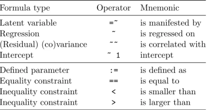
Formula type Operator Mnemonic Latent variable =~ is manifested by Regression ~ is regressed on (Residual) (co)variance ~~ is correlated with

Intercept ~ 1 intercept

Defined parameter := is defined as Equality constraint == is equal to Inequality constraint < is smaller than Inequality constraint > is larger than

Table 1: Top panel of the table contains the four formula types that can be used to specify a model in thelavaanmodel syntax. The lower panel contains additional operators that are allowed in thelavaanmodel syntax.

Finally, intercepts for observed and latent variables are simple regression formulas (using the ‘~’ operator) with only an intercept (explicitly denoted by the number ‘1’) as the only predictor:

item1 ~ 1 # intercept of an observed variable f1 ~ 1 # intercept of a latent variable

Using these fourformula types, a large variety of latent variable models can be described. For reference, we summarize the four formula types in the top panel of Table1.

A typical model syntax describing a SEM model will contain multiple formula types. Inlavaan, to glue them together, they must be specified as a literal string. In theRenvironment, this can be done by enclosing the formula expressions with (single) quotes. For example,

myModel <- '# regressions y ~ f1 + f2 y ~ x1 + x2 f1 ~ x1 + x2 # latent variables

f1 =~ item1 + item2 + item3 f2 =~ item4 + item5 +

item6 + item7 f3 =~ f1 + f2

# (residual) variances and covariances item1 ~~ item1

item1 ~~ item2 # intercepts

item1 ~ 1 f1 ~ 1'

This piece of code will produce a model syntax object calledmyModelthat can be used later when calling a function that estimates this model given a dataset, and it illustrates several

(8)

features of thelavaan model syntax. Formulas can be split over multiple lines, and you can use comments (starting with the ‘#’ character) and blank lines within the single quotes to improve readability of the model syntax. The order in which the formulas are specified does not matter. Therefore, you can use the latent variables in the regression formulas even before they are defined by the ‘=~’ operator. And finally, since this model syntax is nothing more than a literal string, you can type the syntax in a separate text file and use a function like

readLines()to read it in. Alternatively, the text processing infrastructure ofRmay be used to generate the syntax for a variety of models, perhaps when running a large simulation study.

4. A first example: Confirmatory factor analysis

Thelavaanpackage contains a built-in dataset calledHolzingerSwineford1939. We therefore start with loading the lavaanpackage:

R> library("lavaan")

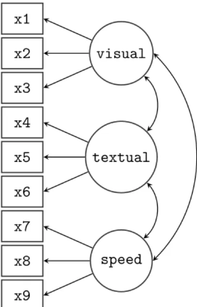
The Holzinger & Swineford 1939 dataset is a ‘classic’ dataset that has been used in many papers and books on structural equation modeling, including some manuals of commercial SEM software packages. The data consists of mental ability test scores of seventh- and eighth-grade children from two different schools (Pasteur and Grant-White). In our version of the dataset, only 9 out of the original 26 tests are included. A CFA model that is often proposed for these 9 variables consists of three correlated latent variables (or factors), each with three indicators:

a visualfactor measured by 3 variables: x1,x2 and x3,

a textual factor measured by 3 variables: x4,x5 andx6,

a speedfactor measured by 3 variables: x7,x8and x9.

x1 x2 x3 x4 x5 x6 x7 x8 x9 visual textual speed

(9)

id lhs op rhs user free ustart 1 visual =~ x1 1 0 1 2 visual =~ x2 1 1 NA 3 visual =~ x3 1 2 NA 4 textual =~ x4 1 0 1 5 textual =~ x5 1 3 NA 6 textual =~ x6 1 4 NA 7 speed =~ x7 1 0 1 8 speed =~ x8 1 5 NA 9 speed =~ x9 1 6 NA 10 x1 ~~ x1 0 7 NA 11 x2 ~~ x2 0 8 NA 12 x3 ~~ x3 0 9 NA 13 x4 ~~ x4 0 10 NA 14 x5 ~~ x5 0 11 NA 15 x6 ~~ x6 0 12 NA 16 x7 ~~ x7 0 13 NA 17 x8 ~~ x8 0 14 NA 18 x9 ~~ x9 0 15 NA 19 visual ~~ visual 0 16 NA 20 textual ~~ textual 0 17 NA 21 speed ~~ speed 0 18 NA 22 visual ~~ textual 0 19 NA 23 visual ~~ speed 0 20 NA 24 textual ~~ speed 0 21 NA

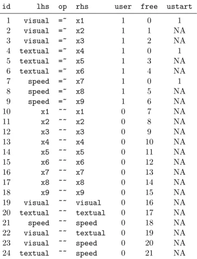
Table 2: A complete list of all parameters in the three-factor CFA model for the Holzinger & Swineford data.

In what follows, we will refer to this 3 factor model as the ‘H&S model’, graphically rep-resented in Figure 1. Note that the path diagram in the figure is simplified: it does not indicate the residual variances of the observed variables or the variances of the exogenous latent variables. Still, it captures the essence of the model. Before discussing the lavaan model syntax for this model, it is worthwhile first to identify the free parameters in this model. There are three latent variables (factors) in this model, each with three indicators, resulting in nine factor loadings that need to be estimated. There are also three covariances among the latent variables – another three parameters. These 12 parameters are represented in the path diagram as single-headed and double-headed arrows, respectively. In addition, however, we need to estimate the residual variances of the nine observed variables and the variances of the latent variables, resulting in 12 additional free parameters. In total we have 24 parameters. But the model is not yet identified because we need to set the metric of the latent variables. There are typically two ways to do this: (1) for each latent variable, fix the factor loading of one of the indicators (typically the first) to a constant (conventionally, 1.0), or (2) standardize the variances of the latent variables. Either way, we fix three of these parameters, and 21 parameters remain free. Table2, produced by the parTable()method, contains an overview of all the relevant parameters for this model, including three fixed factor

(10)

loadings. Each row in the table corresponds to a single parameter. The ‘rhs’, ‘op’ and ‘lhs’ columns uniquely define the parameters of the model. All parameters with the ‘=~’ operator are factor loadings, whereas all parameters with the ‘~~’ operator are variances or covariances. The nonzero elements in the ‘free’ column are the free parameters of the model. The zero elements in the ‘free’ column correspond to fixed parameters, whose value is found in the ‘ustart’ column. The meaning of the ‘user’ column will be explained below.

4.1. Specifying a model using the lavaan model syntax

There are three approaches in lavaan to specify a model. In the first approach, a minimal description of the model is given by the user and the remaining elements are added automat-ically by the program. This ‘user-friendly’ approach is implemented in the fitting functions

cfa() and sem(). In the second approach, a complete explication of all model parameters must be provided by the user – nothing is added automatically. This is the ‘power-user’ ap-proach, implemented in the functionlavaan(). Finally, in a third approach, the minimalist and complete approaches are blended by providing an incomplete description of the model in the model syntax, but adding selected groups of parameters using theauto.* arguments of thelavaan function. We illustrate and discuss each of these approaches in turn.

Method 1: Using the cfa() and sem() functions

In the first approach, the idea is that the model syntax provided by the user should be as concise and intelligible as possible. To accomplish this, typically only the latent variables (using the ‘=~’ operator) and regressions (using the ‘~’ operator) are included in the model syntax. The other model parameters (for this model: the residual variances of the observed variables, the variances of the factors and the covariances among the factors) are added automatically. Since the H&S example contains three latent variables, but no regressions, the minimalist syntax is very short:

R> HS.model <- 'visual =~ x1 + x2 + x3

+ textual =~ x4 + x5 + x6

+ speed =~ x7 + x8 + x9'

We can now fit the model as follows:

R> fit <- cfa(HS.model, data = HolzingerSwineford1939)

The function cfa() is a dedicated function for fitting confirmatory factor analysis (CFA) models. The first argument is the object containing the lavaan model syntax. The second argument is the dataset that contains the observed variables. The ‘user’ column in Table 2

shows which parameters were explicitly contained in the user-specified model syntax (= 1), and which parameters were added by thecfa() function (= 0). If a model has been fitted, it is always possible (and highly informative) to inspect this parameter table by using the following command:

parTable(fit)

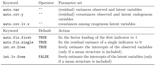
When using the cfa() (or sem()) function, several sets of parameters are included by de-fault. A complete list of these parameter sets is provided in the top panel of Table 3. In

(11)

Keyword Operator Parameter set

auto.var ~~ (residual) variances observed and latent variables

auto.cov.y ~~ (residual) covariances observed and latent endogenous variables

auto.cov.lv.x ~~ covariances among exogenous latent variables Keyword Default Action

auto.fix.first TRUE fix the factor loading of the first indicator to 1

auto.fix.single TRUE fix the residual variance of a single indicator to 0

int.ov.free TRUE freely estimate the intercepts of the observed variables (only if a mean structure is included)

int.lv.free FALSE freely estimate the intercepts of the latent variables (only if a mean structure is included)

Table 3: Top panel: Sets of parameters that are automatically added to the model repre-sentation when the functions cfa() or sem() are used. Bottom panel: The set of actions automatically taken in an attempt to fulfill the minimum requirements for an identifiable model. These defaults are used by thecfa()orsem()functions only.

addition, several steps are taken in an attempt to fulfill the minimum requirements for an identifiable model. These steps are listed in the bottom panel of Table3. In our example, only the first action (fixing the factor loadings of the first indicator) is used. The second one (auto.fix.single) is only needed if the model contains a latent variable that is manifested by a single indicator. The third and the fourth actions (int.ov.free and int.lv.free, respectively) are only needed if a mean structure is added to the model.

Before we move on to the next method, it is important to stress that all of these ‘automatic’ actions can be overridden. The model syntax always has precedence over the automatically generated actions. If, for example, one wishes not to fix the factor loadings of the first indicator, but instead to fix the variances of the latent variances, the model syntax would be adapted as follows:

R> HS.model.bis <- 'visual =~ NA*x1 + x2 + x3

+ textual =~ NA*x4 + x5 + x6

+ speed =~ NA*x7 + x8 + x9

+ visual ~~ 1*visual

+ textual ~~ 1*textual

+ speed ~~ 1*speed'

As illustrated above, model parameters are fixed by pre-multiplying them with a numeric value, and otherwise fixed parameters are freed by pre-multiplying them with ‘NA’. The model syntax above overrides the default behavior of fixing the first factor loading and es-timating the factor variances. In practice, however, a much more convenient method to use this parameterization is to keep the original syntax, but add thestd.lv = TRUE argument to thecfa()function call:

(12)

Method 2: Using the lavaan() function

In many situations, using the concise model syntax in combination with the cfa()andsem()

functions is extremely convenient, particularly for many conventional models. But sometimes, these automatic actions may get in the way, especially when non-standard models need to be specified. For these situations, users may prefer to use thelavaan() function instead. The

lavaan()function has the ‘feature’ that it does not add any extra parameters to the model by default, nor does it attempt to make the model identifiable. If the lavaan()function is called without any use of theauto.*arguments, it becomes the user’s responsibility to specify the correct model syntax. This can lead to lengthier model specifications, but the user has full control. For the H&S model, the fulllavaanmodel syntax would be:

R> HS.model.full <- '# latent variables

+ visual =~ 1*x1 + x2 + x3

+ textual =~ 1*x4 + x5 + x6

+ speed =~ 1*x7 + x8 + x9

+ # residual variances observed variables

+ x1 ~~ x1 + x2 ~~ x2 + x3 ~~ x3 + x4 ~~ x4 + x5 ~~ x5 + x6 ~~ x6 + x7 ~~ x7 + x8 ~~ x8 + x9 ~~ x9 + # factor variances + visual ~~ visual + textual ~~ textual + speed ~~ speed + # factor covariances

+ visual ~~ textual + speed

+ textual ~~ speed'

R> fit <- lavaan(HS.model.full, data = HolzingerSwineford1939)

Method 3: Using the lavaan() function with the auto.* arguments

When using thelavaan()function, the user has full control, but the model syntax may be-come long and contain many formulas that could easily be added automatically. To compro-mise between a complete model specification usinglavaansyntax and the automatic addition of certain parameters, thelavaan()function provides several optional arguments that can be used to add a particular set of parameters to the model, or to fix a particular set of parameters (see Table 3). For example, in the model syntax below, the first factor loadings are explicitly fixed to one, and the covariances among the factors are added manually. It would be more convenient and concise, however, to omit the residual variances and factor variances from the model syntax. The following model syntax and call to lavaan()achieves this:

(13)

R> HS.model.mixed <- '# latent variables

+ visual =~ 1*x1 + x2 + x3

+ textual =~ 1*x4 + x5 + x6

+ speed =~ 1*x7 + x8 + x9

+ # factor covariances

+ visual ~~ textual + speed

+ textual ~~ speed'

R> fit <- lavaan(HS.model.mixed, data = HolzingerSwineford1939,

+ auto.var = TRUE)

4.2. Examining the results

All three methods described above fit the same model. The cfa(), sem() and lavaan()

fitting functions all return an object of class “lavaan”, for which several methods are available to examine model fit statistics and parameters estimates. Table 4 contains an overview of some of these methods.

The summary() method

Perhaps the most useful method to view results from a SEM fitted with lavaanissummary(). The summary() method can be called without any extra arguments, in which case only a short description of the model fit is displayed, together with the parameter estimates. Some extra arguments of the summary()method are fit.measures,standardized, and rsquare.

Method Description

summary() print a long summary of the model results

show() print a short summary of the model results

coef() returns the estimates of the free parameters in the model as a named numeric vector

fitted() returns the implied moments (covariance matrix and mean vector) of the model

resid() returns the raw, normalized or standardized residuals (difference between implied and observed moments)

vcov() returns the covariance matrix of the estimated parameters

predict() compute factor scores

logLik() returns the log-likelihood of the fitted model (if maximum likelihood es-timation was used)

AIC(),BIC() compute information criteria (if maximum likelihood estimation was used)

update() update a fittedlavaan object

inspect() peek into the internal representation of the model; by default, it returns a list of model matrices counting the free parameters in the model; can also be used to extract starting values, gradient values, and much more Table 4: Some methods for objects of class “lavaan”. See the help page for the lavaan class for more details (typeclass?lavaan at theRprompt).

(14)

If one or more of these is set to TRUE, the output will be enriched with additional fit mea-sures, standardized estimates, andR2 values for the dependent variables, respectively. In the example below, we request only the additional fit measures.

+ speed =~ x7 + x8 + x9'

R> fit <- cfa(HS.model, data = HolzingerSwineford1939) R> summary(fit, fit.measures = TRUE)

lavaan (0.4-14) converged normally after 41 iterations

Number of observations 301

Estimator ML

Minimum Function Chi-square 85.306

Degrees of freedom 24

P-value 0.000

Chi-square test baseline model:

P-value 0.000

Full model versus baseline model:

Comparative Fit Index (CFI) 0.931

Tucker-Lewis Index (TLI) 0.896

Loglikelihood and Information Criteria:

Loglikelihood user model (H0) -3737.745

Loglikelihood unrestricted model (H1) -3695.092

Number of free parameters 21

Akaike (AIC) 7517.490

Bayesian (BIC) 7595.339

Sample-size adjusted Bayesian (BIC) 7528.739

Root Mean Square Error of Approximation:

RMSEA 0.092

90 Percent Confidence Interval 0.071 0.114

P-value RMSEA <= 0.05 0.001

(15)

SRMR 0.065 Parameter estimates:

Information Expected

Standard Errors Standard

Estimate Std.err Z-value P(>|z|) Latent variables: visual =~ x1 1.000 x2 0.553 0.100 5.554 0.000 x3 0.729 0.109 6.685 0.000 textual =~ x4 1.000 x5 1.113 0.065 17.014 0.000 x6 0.926 0.055 16.703 0.000 speed =~ x7 1.000 x8 1.180 0.165 7.152 0.000 x9 1.082 0.151 7.155 0.000 Covariances: visual ~~ textual 0.408 0.074 5.552 0.000 speed 0.262 0.056 4.660 0.000 textual ~~ speed 0.173 0.049 3.518 0.000 Variances: x1 0.549 0.114 x2 1.134 0.102 x3 0.844 0.091 x4 0.371 0.048 x5 0.446 0.058 x6 0.356 0.043 x7 0.799 0.081 x8 0.488 0.074 x9 0.566 0.071 visual 0.809 0.145 textual 0.979 0.112 speed 0.384 0.086

The output consists of three sections. The first section (the first 6 lines) contains the package version number, an indication whether the model has converged (and in how many iterations), and the effective number of observations used in the analysis. Next, the modelχ2test statistic,

(16)

degrees of freedom, and a p value are printed. If fit.measures = TRUE, a second section is printed containing the test statistic of the baseline model (where all observed variables are assumed to be uncorrelated) and several popular fit indices. If maximum likelihood estimation is used, this section will also contain information about the loglikelihood, the AIC, and the BIC. The third section provides an overview of the parameter estimates, including the type of standard errors used and whether the observed or expected information matrix was used to compute standard errors. Then, for each model parameter, the estimate and the standard error are displayed, and if appropriate, azvalue based on the Wald test and a corresponding two-sided p value are also shown. To ease the reading of the parameter estimates, they are grouped into three blocks: (1) factor loadings, (2) factor covariances, and (3) (residual) variances of both observed variables and factors.

TheparameterEstimates() method

Although thesummary() method provides a nice summary of the model results, it is useful for display only. An alternative is the parameterEstimates() method, which returns the parameter estimates as a data.frame, making the information easily accessible for further processing. By default, theparameterEstimates()method includes the estimates, standard errors,zvalue, p value, and 95% confidence intervals for all the model parameters.

R> parameterEstimates(fit)

lhs op rhs est se z pvalue ci.lower ci.upper

1 visual =~ x1 1.000 0.000 NA NA 1.000 1.000 2 visual =~ x2 0.553 0.100 5.554 0 0.358 0.749 3 visual =~ x3 0.729 0.109 6.685 0 0.516 0.943 4 textual =~ x4 1.000 0.000 NA NA 1.000 1.000 5 textual =~ x5 1.113 0.065 17.014 0 0.985 1.241 6 textual =~ x6 0.926 0.055 16.703 0 0.817 1.035 7 speed =~ x7 1.000 0.000 NA NA 1.000 1.000 8 speed =~ x8 1.180 0.165 7.152 0 0.857 1.503 9 speed =~ x9 1.082 0.151 7.155 0 0.785 1.378 10 x1 ~~ x1 0.549 0.114 4.833 0 0.326 0.772 11 x2 ~~ x2 1.134 0.102 11.146 0 0.934 1.333 12 x3 ~~ x3 0.844 0.091 9.317 0 0.667 1.022 13 x4 ~~ x4 0.371 0.048 7.779 0 0.278 0.465 14 x5 ~~ x5 0.446 0.058 7.642 0 0.332 0.561 15 x6 ~~ x6 0.356 0.043 8.277 0 0.272 0.441 16 x7 ~~ x7 0.799 0.081 9.823 0 0.640 0.959 17 x8 ~~ x8 0.488 0.074 6.573 0 0.342 0.633 18 x9 ~~ x9 0.566 0.071 8.003 0 0.427 0.705 19 visual ~~ visual 0.809 0.145 5.564 0 0.524 1.094 20 textual ~~ textual 0.979 0.112 8.737 0 0.760 1.199 21 speed ~~ speed 0.384 0.086 4.451 0 0.215 0.553 22 visual ~~ textual 0.408 0.074 5.552 0 0.264 0.552 23 visual ~~ speed 0.262 0.056 4.660 0 0.152 0.373 24 textual ~~ speed 0.173 0.049 3.518 0 0.077 0.270

(17)

The confidence level can be changed by setting thelevelargument. Settingci = FALSE sup-presses the confidence intervals. Another use of this function is to obtain several standardized versions of the estimates, by settingstandardized = TRUE:

R> Est <- parameterEstimates(fit, ci = FALSE, standardized = TRUE) R> subset(Est, op == "=~")

lhs op rhs est se z pvalue std.lv std.all std.nox

1 visual =~ x1 1.000 0.000 NA NA 0.900 0.772 0.772 2 visual =~ x2 0.553 0.100 5.554 0 0.498 0.424 0.424 3 visual =~ x3 0.729 0.109 6.685 0 0.656 0.581 0.581 4 textual =~ x4 1.000 0.000 NA NA 0.990 0.852 0.852 5 textual =~ x5 1.113 0.065 17.014 0 1.102 0.855 0.855 6 textual =~ x6 0.926 0.055 16.703 0 0.917 0.838 0.838 7 speed =~ x7 1.000 0.000 NA NA 0.619 0.570 0.570 8 speed =~ x8 1.180 0.165 7.152 0 0.731 0.723 0.723 9 speed =~ x9 1.082 0.151 7.155 0 0.670 0.665 0.665

Here, only the factor loadings are shown. Relative to the prior output, three columns with standardized values were added. In the first column (std.lv), only the latent variables have been standardized; in the second column (std.all), both the latent and the observed variables have been standardized; in the third column (std.nox), both the latent and the observed variables have been standardized, except for the exogenous observed variables. The last of these options may be useful if the standardization of exogenous observed variables has little meaning (for example, binary covariates). Since there are no exogenous covariates in this model, the last two columns are identical in this output.

ThemodificationIndices() method

If the model fit is not superb, it may be informative to inspect the modification indices (MIs) and their corresponding expected parameter changes (EPCs). In essence, modification indices provide a rough estimate of how theχ2test statistic of a model would improve, if a particular parameter were unconstrained. The expected parameter change is the value this parameter would have if it were included as a free parameter. ThemodificationIndices()method (or the alias with the shorter name, modindices()) will print out a long list of parameters as a

data.frame. In the output below, we only show those parameters for which the modification index is 10 or higher.

R> MI <- modificationIndices(fit) R> subset(MI, mi > 10)

lhs op rhs mi epc sepc.lv sepc.all sepc.nox 1 visual =~ x7 18.631 -0.422 -0.380 -0.349 -0.349

2 visual =~ x9 36.411 0.577 0.519 0.515 0.515

3 x7 ~~ x8 34.145 0.536 0.536 0.488 0.488

4 x8 ~~ x9 14.946 -0.423 -0.423 -0.415 -0.415

The last three columns contain the standardized EPCs, using the same standardization con-ventions as for ordinary parameter estimates.

(18)

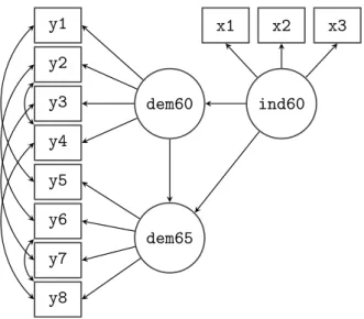
y1 y2 y3 y4 y5 y6 y7 y8 x1 x2 x3 dem60 dem65 ind60

Figure 2: Path diagram of the structural equation model used to fit the Political Democracy data.

5. A second example: Structural equation modeling

In our second example, we will explore the ‘Industrialization and Political Democracy’ dataset previously used by Bollen in his 1989 book on structural equation modeling (Bollen 1989), and included with lavaan in the PoliticalDemocracy data.frame. The dataset contains various measures of political democracy and industrialization in developing countries. In the model, three latent variables are defined. The focus of the analysis is on the structural part of the model (i.e., the regressions among the latent variables). A graphical representation of the model is depicted in Figure2.

5.1. Specifying and fitting the model, examining the results

For this example, we will only use the user-friendlysem()function to keep the model syntax as concise as possible. To describe the model, we need three different formula types: latent variables, regression formulas, and (co)variance formulas for the residual covariances among the observed variables. After the model has been fitted, we request a summary with no fit measures, but with standardized parameter estimates.

R> model <- ' + # measurement model + ind60 =~ x1 + x2 + x3 + dem60 =~ y1 + y2 + y3 + y4 + dem65 =~ y5 + y6 + y7 + y8 + # regressions + dem60 ~ ind60

+ dem65 ~ ind60 + dem60

+ # residual covariances

+ y1 ~~ y5

+ y2 ~~ y4 + y6

(19)

+ y4 ~~ y8

+ y6 ~~ y8'

R> fit <- sem(model, data = PoliticalDemocracy) R> summary(fit, standardized = TRUE)

Estimator ML

P-value 0.329

Parameter estimates:

Estimate Std.err Z-value P(>|z|) Std.lv Std.all Latent variables: ind60 =~ x1 1.000 0.670 0.920 x2 2.180 0.139 15.742 0.000 1.460 0.973 x3 1.819 0.152 11.967 0.000 1.218 0.872 dem60 =~ y1 1.000 2.223 0.850 y2 1.257 0.182 6.889 0.000 2.794 0.717 y3 1.058 0.151 6.987 0.000 2.351 0.722 y4 1.265 0.145 8.722 0.000 2.812 0.846 dem65 =~ y5 1.000 2.103 0.808 y6 1.186 0.169 7.024 0.000 2.493 0.746 y7 1.280 0.160 8.002 0.000 2.691 0.824 y8 1.266 0.158 8.007 0.000 2.662 0.828 Regressions: dem60 ~ ind60 1.483 0.399 3.715 0.000 0.447 0.447 dem65 ~ ind60 0.572 0.221 2.586 0.010 0.182 0.182 dem60 0.837 0.098 8.514 0.000 0.885 0.885 Covariances: y1 ~~ y5 0.624 0.358 1.741 0.082 0.624 0.296 y2 ~~

(20)

y4 1.313 0.702 1.871 0.061 1.313 0.273 y6 2.153 0.734 2.934 0.003 2.153 0.356 y3 ~~ y7 0.795 0.608 1.308 0.191 0.795 0.191 y4 ~~ y8 0.348 0.442 0.787 0.431 0.348 0.109 y6 ~~ y8 1.356 0.568 2.386 0.017 1.356 0.338 Variances: x1 0.082 0.019 0.082 0.154 x2 0.120 0.070 0.120 0.053 x3 0.467 0.090 0.467 0.239 y1 1.891 0.444 1.891 0.277 y2 7.373 1.374 7.373 0.486 y3 5.067 0.952 5.067 0.478 y4 3.148 0.739 3.148 0.285 y5 2.351 0.480 2.351 0.347 y6 4.954 0.914 4.954 0.443 y7 3.431 0.713 3.431 0.322 y8 3.254 0.695 3.254 0.315 ind60 0.448 0.087 1.000 1.000 dem60 3.956 0.921 0.800 0.800 dem65 0.172 0.215 0.039 0.039

5.2. Parameter labels and simple equality constraints

Inlavaan, each parameter has a name, referred to as the ‘parameter label’. The naming scheme is automatic and follows a simple set of rules. Each label consists of three components that describe the relevant formula defining the parameter. The first part is the variable name that appears on the left-hand side of the formula operator. The second part is the operator type of the formula, and the third part is the variable on the right-hand side of the operator that corresponds with the parameter. To see the naming mechanism in action, we can use the coef() function, which returns the (estimated) values of the free parameters and their corresponding parameter labels.

R> coef(fit)

ind60=~x2 ind60=~x3 dem60=~y2 dem60=~y3 dem60=~y4 dem65=~y6

2.180 1.819 1.257 1.058 1.265 1.186

dem65=~y7 dem65=~y8 dem60~ind60 dem65~ind60 dem65~dem60 y1~~y5

1.280 1.266 1.483 0.572 0.837 0.624

y2~~y4 y2~~y6 y3~~y7 y4~~y8 y6~~y8 x1~~x1

1.313 2.153 0.795 0.348 1.356 0.082

x2~~x2 x3~~x3 y1~~y1 y2~~y2 y3~~y3 y4~~y4

(21)

y5~~y5 y6~~y6 y7~~y7 y8~~y8 ind60~~ind60 dem60~~dem60

2.351 4.954 3.431 3.254 0.448 3.956

dem65~~dem65 0.172

Custom labels may be provided by the user in the model syntax, by pre-multiplying a variable name with that label. Consider, for example, the following regression formula:

y ~ b1*x1 + b2*x2 + b3*x3 + b4*x4

Here we have ‘named’ or ‘labeled’ the four regression coefficients asb1,b2,b3andb4. Custom labels are convenient because you can refer to them in other places of the model syntax. In particular, labels can be used to impose equality constraints on certain parameters. If two parameters have the same name, they will be considered to be the same, and only one value will be computed for them (i.e., a simple equality constraint). To illustrate this, we will respecify the model syntax of the Political Democracy data. In the original example in Bollen’s book, the factor loadings of the dem60 factor are constrained to be equal to the factor loadings of the dem65 factor. This make sense, since it is the same construct that is measured on two time points. To enforce these equality constraints, we label the factor loadings of the dem60

factor (arbitrarily) asd1,d2, and d3. Note that we do not label the first factor loading since it is a fixed parameter (equal to 1.0). Next, we use the same labels for the factor loadings of the dem65factor, effectively imposing three equality constraints.

R> model.equal <- '# measurement model

+ ind60 =~ x1 + x2 + x3

+ dem60 =~ y1 + d1*y2 + d2*y3 + d3*y4

+ dem65 =~ y5 + d1*y6 + d2*y7 + d3*y8

+ # regressions

+ dem60 ~ ind60

+ dem65 ~ ind60 + dem60

+ # residual covariances + y1 ~~ y5 + y2 ~~ y4 + y6 + y3 ~~ y7 + y4 ~~ y8 + y6 ~~ y8'

R> fit.equal <- sem(model.equal, data = PoliticalDemocracy) R> summary(fit.equal)

Estimator ML

(22)

Estimate Std.err Z-value P(>|z|) Latent variables: ind60 =~ x1 1.000 x2 2.180 0.138 15.751 0.000 x3 1.818 0.152 11.971 0.000 dem60 =~ y1 1.000 y2 (d1) 1.191 0.139 8.551 0.000 y3 (d2) 1.175 0.120 9.755 0.000 y4 (d3) 1.251 0.117 10.712 0.000 dem65 =~ y5 1.000 y6 (d1) 1.191 0.139 8.551 0.000 y7 (d2) 1.175 0.120 9.755 0.000 y8 (d3) 1.251 0.117 10.712 0.000 Regressions: dem60 ~ ind60 1.471 0.392 3.750 0.000 dem65 ~ ind60 0.600 0.226 2.661 0.008 dem60 0.865 0.075 11.554 0.000 Covariances: y1 ~~ y5 0.583 0.356 1.637 0.102 y2 ~~ y4 1.440 0.689 2.092 0.036 y6 2.183 0.737 2.960 0.003 y3 ~~ y7 0.712 0.611 1.165 0.244 y4 ~~ y8 0.363 0.444 0.817 0.414 y6 ~~ y8 1.372 0.577 2.378 0.017 Variances: x1 0.081 0.019 x2 0.120 0.070 x3 0.467 0.090

(23)

y1 1.855 0.433 y2 7.581 1.366 y3 4.956 0.956 y4 3.225 0.723 y5 2.313 0.479 y6 4.968 0.921 y7 3.560 0.710 y8 3.308 0.704 ind60 0.449 0.087 dem60 3.875 0.866 dem65 0.164 0.227

The fit of the constrained model is slightly worse compared to the unconstrained model. But is it significantly worse? To compare two nested models, we can use the anova() function, which will compute theχ2 difference test:

R> anova(fit, fit.equal)

Chi Square Difference Test

Df AIC BIC Chisq Chisq diff Df diff Pr(>Chisq)

fit 35 3157.6 3229.4 38.125

fit.equal 38 3153.6 3218.5 40.179 2.0543 3 0.5612

5.3. Extracting fit measures

The summary() method with the argument fit.measures = TRUE will output a number of fit measures. If fit statistics are needed for further processing, thefitMeasures() method is preferred. The first argument tofitMeasures() is the fitted object and the second argument is a character vector containing the names of the fit measures one wish to extract. For example, if we only need the CFI and RMSEA values, we can use:

R> fitMeasures(fit, c("cfi", "rmsea"))

cfi rmsea 0.995 0.035

Omitting the second argument will return all the fit measures computed bylavaan. 5.4. Using the inspect() method

To finish our SEM example, we will briefly mention theinspect() method which allows the user to peek under the hood of a lavaan object. By default, calling inspect() on a fitted lavaan object returns a list of the model matrices that are used internally to represent the model. The free parameters are nonzero integers.

(24)

$lambda

ind60 dem60 dem65

x1 0 0 0 x2 1 0 0 x3 2 0 0 y1 0 0 0 y2 0 3 0 y3 0 4 0 y4 0 5 0 y5 0 0 0 y6 0 0 6 y7 0 0 7 y8 0 0 8 $theta x1 x2 x3 y1 y2 y3 y4 y5 y6 y7 y8 x1 18 x2 0 19 x3 0 0 20 y1 0 0 0 21 y2 0 0 0 0 22 y3 0 0 0 0 0 23 y4 0 0 0 0 13 0 24 y5 0 0 0 12 0 0 0 25 y6 0 0 0 0 14 0 0 0 26 y7 0 0 0 0 0 15 0 0 0 27 y8 0 0 0 0 0 0 16 0 17 0 28 $psi

ind60 dem60 dem65 ind60 29

dem60 0 30

dem65 0 0 31

$beta

ind60 dem60 dem65

ind60 0 0 0

dem60 9 0 0

dem65 10 11 0

The output reveals that lavaan is currently using the LISREL matrix representation, albeit with no distinction between endogenous and exogenous variables. This is the so-called ‘all-y’ representation. In future releases, I plan to allow for alternative matrix representations, including the Bentler-Weeks and the reticular action model (RAM) approach (Bollen 1989, chapter 9). To see the starting values of the parameters in each model matrix, type

(25)

$lambda

ind60 dem60 dem65 x1 1.000 0.000 0.000 x2 2.193 0.000 0.000 x3 1.824 0.000 0.000 y1 0.000 1.000 0.000 y2 0.000 1.296 0.000 y3 0.000 1.055 0.000 y4 0.000 1.294 0.000 y5 0.000 0.000 1.000 y6 0.000 0.000 1.303 y7 0.000 0.000 1.403 y8 0.000 0.000 1.401 $theta x1 x2 x3 y1 y2 y3 y4 y5 y6 y7 y8 x1 0.265 x2 0.000 1.126 x3 0.000 0.000 0.975 y1 0.000 0.000 0.000 3.393 y2 0.000 0.000 0.000 0.000 7.686 y3 0.000 0.000 0.000 0.000 0.000 5.310 y4 0.000 0.000 0.000 0.000 0.000 0.000 5.535 y5 0.000 0.000 0.000 0.000 0.000 0.000 0.000 3.367 y6 0.000 0.000 0.000 0.000 0.000 0.000 0.000 0.000 5.612 y7 0.000 0.000 0.000 0.000 0.000 0.000 0.000 0.000 0.000 5.328 y8 0.000 0.000 0.000 0.000 0.000 0.000 0.000 0.000 0.000 0.000 5.197 $psi

ind60 dem60 dem65 ind60 0.05

dem60 0.00 0.05

dem65 0.00 0.00 0.05 $beta

ind60 dem60 dem65

ind60 0 0 0

dem60 0 0 0

dem65 0 0 0

Many more inspect options are described in the help page for thelavaan class.

6. Multiple groups

The lavaanpackage has full support for multiple-groups SEM. To request a multiple-groups analysis, the variable defining group membership in the dataset can be passed to the group

(26)

argument of the cfa(), sem(), or lavaan() function calls. By default, the same model is fitted in all groups without any equality constraints on the model parameters. In the following example, we fit the H&S model for the two schools (Pasteur and Grant-White).

+ speed =~ x7 + x8 + x9'

R> fit <- cfa(HS.model, data = HolzingerSwineford1939, group = "school")

The summary() output is rather long and not shown here. Essentially, it shows a set of parameter estimates for the Pasteur group, followed by another set of parameter estimates for the Grant-White group. If we wish to impose equality constraints on model parame-ters across groups, we can use the group.equal argument. For example, group.equal = c("loadings", "intercepts")will constrain both the factor loadings and the intercepts of the observed variables to be equal across groups. Other options that can be included in the

group.equal argument are described in the help pages of the fitting functions. As a short example, we will fit the H&S model for the two schools, but constrain the factor loadings and intercepts to be equal. Theanovafunction can be used to compare the two model fits.

R> fit.metric <- cfa(HS.model, data = HolzingerSwineford1939,

+ group = "school", group.equal = c("loadings", "intercepts"))

R> anova(fit, fit.metric)

Chi Square Difference Test

Df AIC BIC Chisq Chisq diff Df diff Pr(>Chisq)

fit 48 7484.4 7706.8 115.85

fit.metric 60 7508.6 7686.6 164.10 48.251 12 2.826e-06

If the group.equal argument is used to constrain the factor loadings across groups, all fac-tor loadings are affected. If some exceptions are needed, one can use the group.partial

argument, which takes a vector of parameter labels that specify which parameters will re-main free across groups. Therefore, the combination of thegroup.equalandgroup.partial

arguments gives the user a flexible mechanism to specify across group equality constraints.

7. Can

lavaan

do this? A short feature list

Thelavaanpackage has many features, and we foresee that the feature list will keep growing in the next couple of years. To present the reader a flavor of the current capabilities oflavaan, I will use this section to mention briefly a variety of topics that are often of interest to users of SEM software.

7.1. Non-normal and categorical data

The 0.4 version of thelavaanpackage only supports continuous data. Support for categorical data is expected in the 0.5 release. In the current release, however, I have devoted considerable attention to dealing with non-normal continuous data. In the SEM literature, the topic of

(27)

dealing with non-normal data is well studied (seeFinney and DiStefano 2006, for an overview). Three popular strategies to deal with non-normal data have been implemented in thelavaan package: asymptotically distribution-free estimation; scaled test statistics and robust standard errors; and bootstrapping.

Asymptotically distribution-free (ADF) estimation

The asymptotically distribution-free (ADF) estimator (Browne 1984) makes no assumption of normality. Therefore, variables that are skewed or kurtotic do not distort the ADF based standard errors and test statistic. The ADF estimator is part of a larger family of estimators called weighted least squares (WLS) estimators. The discrepancy function of these estimators can be written as follows:

F = (s−σˆ)>W−1(s−σˆ)

where s is a vector of the non-duplicated elements in the sample covariance matrix (S), ˆσ is a vector of the non-duplicated elements of the model-implied covariance matrix ( ˆΣ), and W is a weight matrix. The weight matrix utilized with the ADF estimator is the asymp-totic covariance matrix: a matrix of the covariances of the observed sample variances and covariances. Theoretically, the ADF estimator seems to be a perfect strategy to deal with non-normal data. Unfortunately, empirical research (e.g., Olsson, Foss, Troye, and Howell 2000) has shown that the ADF method breaks down unless the sample size is huge (e.g.,

N >5000).

In lavaan, the estimator can be set by using the estimator argument in one of the fitting functions. The default is maximum likelihood estimation, orestimator = "ML". To switch to the ADF estimator, you can setestimator = "WLS".

Satorra-Bentler scaled test statistic and robust standard errors

An alternative strategy is to use maximum likelihood (ML) for estimating the model param-eters, even if the data are known to be non-normal. In this case, the parameter estimates are still consistent (if the model is identified and correctly specified), but the standard errors tend to be too small (as much as 25–50%), meaning that we may reject the null hypothesis (that a parameter is zero) too often. In addition, the model (χ2) test statistic tends to be too large, meaning that we may reject the model too often.

In the SEM literature, several authors have extended the ML methodology to produce stan-dard errors that are asymptotically correct for arbitrary distributions (with finite fourth-order moments), and where a rescaled test statistic is used for overall model evaluation.

Standard errors of the maximum likelihood estimators are based on the covariance matrix that is obtained by inverting the associated information matrix. Robust standard errors replace this covariance matrix by a sandwich-type covariance matrix, first proposed byHuber

(1967) and introduced in the SEM literature byBentler (1983);Browne (1984);Browne and Arminger(1995) and many others. Inlavaan, theseargument can be used to switch between different types of standard errors. Settingse = "robust"will produce robust standard errors based on a sandwich-type covariance matrix.

The best known method for correcting the model test statistic is the so-called Satorra-Bentler scaled test statistic (Satorra and Bentler 1988, 1994). Their method rescales the value of the ML-based χ2 test statistic by an amount that reflects the degree of kurtosis. Several

(28)

simulation studies have shown that this correction is effective with non-normal data (Chou, Bentler, and Satorra 1991;Curran, West, and Finch 1996), even in small to moderate samples. And because applying the correction often results in a better model fit, it is not surprising that the Satorra-Bentler rescaling method has become popular among SEM users.

Inlavaan, thetest argument can be used to switch between different test statistics. Setting

test = "satorra.bentler"supplements the standardχ2 model test with the scaled version. In the output produced by thesummary()method, both scaled and unscaled model tests (and corresponding fit indices) are displayed in adjacent columns. Because one typically wants both robust standard errors and a scaled test statistic, specifying estimator = "MLM" fits the model using standard maximum likelihood to estimate the model parameters, but with robust standard errors and a Satorra-Bentler scaled test statistic.

R> fit <- cfa(HS.model, data = HolzingerSwineford1939, missing = "listwise",

+ estimator = "MLM", mimic = "Mplus")

R> summary(fit, estimates = FALSE, fit.measures = TRUE)

Estimator ML Robust

Minimum Function Chi-square 85.306 81.908

Degrees of freedom 24 24

P-value 0.000 0.000

Scaling correction factor 1.041

for the Satorra-Bentler correction (Mplus variant) Chi-square test baseline model:

P-value 0.000 0.000

Full model versus baseline model:

Comparative Fit Index (CFI) 0.931 0.932

Tucker-Lewis Index (TLI) 0.896 0.898

Loglikelihood and Information Criteria:

Loglikelihood user model (H0) -3737.745 -3737.745

Loglikelihood unrestricted model (H1) -3695.092 -3695.092

Number of free parameters 30 30

Akaike (AIC) 7535.490 7535.490

Bayesian (BIC) 7646.703 7646.703

(29)

Root Mean Square Error of Approximation:

RMSEA 0.092 0.090

90 Percent Confidence Interval 0.071 0.114 0.069 0.111

P-value RMSEA <= 0.05 0.001 0.001

Standardized Root Mean Square Residual:

SRMR 0.060 0.060

In this example, the mimic = "Mplus" argument was used to mimic the way the Mplus program computes the Satorra-Bentler scaled test statistic. By default (i.e., when themimic

argument is omitted),lavaanwill use the method that is used by theEQSprogram. To mimic the exact value of the Satorra-Bentler scaled test statistic as reported by the EQSprogram, one can use

R> fit <- cfa(HS.model, data = HolzingerSwineford1939, estimator = "MLM",

+ mimic = "EQS")

R> fit

Estimator ML Robust

P-value 0.000 0.000

Scaling correction factor 1.048

for the Satorra-Bentler correction

If two models are nested, but the model test statistics are scaled, the usual χ2 difference test can no longer be used. Instead, a special procedure is needed known as the scaled χ2

difference test (Satorra and Bentler 2001). Theanova()function inlavaanwill automatically detect this and compute a scaled χ2 _{difference test if appropriate.}

Bootstrapping: The na¨ıve bootstrap and the Bollen-Stine bootstrap

The third strategy for dealing with non-normal data is bootstrapping. For standard errors, we can use the standard nonparametric bootstrap to obtain bootstrap standard errors. However, to bootstrap the test statistic (and its p value), the standard (na¨ıve) bootstrap is incorrect because it reflects not only non-normality and sampling variability, but also model misfit. Therefore, the original sample must first be transformed so that the sample covariance matrix corresponds with the model-implied covariance. In the SEM literature, this model-based bootstrap procedure is known as the Bollen-Stine bootstrap (Bollen and Stine 1993).

In lavaan, bootstrap standard errors can be obtained by setting se = "bootstrap". In this case, the confidence intervals produced by the parameterEstimates() method will be

(30)

bootstrap-based confidence intervals. If test = "bootstrap" or test = "bollen.stine", the data are first transformed to perform a model-based ‘Bollen-Stine’ bootstrap. The boot-strap standard errors are also based on these model-based bootboot-strap draws, and the standard

p value of the χ2 test statistic is supplemented with a bootstrap probability value, obtained by computing the proportion of test statistics from the bootstrap samples that exceed the value of the test statistic from the original (parent) sample.

By default,lavaangenerates R= 1000 bootstrap draws, but this number can be changed by setting thebootstrap argument. It may be informative to set verbose = TRUE to monitor the progress of bootstrapping.

7.2. Missing data

If the data contain missing values, the default behavior in lavaan is listwise deletion. If the missing mechanism is MCAR (missing completely at random) or MAR (missing at random), the lavaan package provides case-wise (or ‘full information’) maximum likelihood (FIML) estimation (Arbuckle 1996). FIML estimation can be enabled by specifying the argument

missing = "ml" (or its alias missing = "fiml") when calling the fitting function. An un-restricted (h1) model will automatically be estimated, so that all common fit indices are available. Robust standard errors are also available, as is a scaled test statistic (Yuan and Bentler 2000) if the data are both incomplete and non-normal.

7.3. Linear and nonlinear equality and inequality constraints

In many applications, it is necessary to impose constraints on some of the model parameters. For example, one may wish to enforce that a variance parameter is strictly positive. For some models, it is important to specify that a parameter is equal to some (linear or nonlinear) function of other parameters. The aim of thelavaanpackage is to make such constraints easy to specify using the lavaan model syntax. A short example will illustrate constraint syntax inlavaan. Consider the following regression:

y ~ b1*x1 + b2*x2 + b3*x3

where we have explicitly labeled the regression coefficients as b1, b2 and b3. We create a toy dataset containing these four variables and fit the regression model:

R> set.seed(1234)

R> Data <- data.frame(y = rnorm(100), x1 = rnorm(100), x2 = rnorm(100),

+ x3 = rnorm(100))

R> model <- 'y ~ b1*x1 + b2*x2 + b3*x3'

R> fit <- sem(model, data = Data) R> coef(fit)

b1 b2 b3 y~~y

-0.052 0.084 0.139 0.970

Suppose that we wish to impose two (nonlinear) constraints on b1: b1 = (b2 +b3)2 and

b1 ≥ exp(b2 +b3). The first constraint is an equality constraint, whereas the second is an inequality constraint. Both constraints are nonlinear. In lavaan, this is accomplished as follows:

(31)

R> model.constr <- '# model with labeled parameters

+ y ~ b1*x1 + b2*x2 + b3*x3

+ # constraints

+ b1 == (b2 + b3)^2

+ b1 > exp(b2 + b3)'

R> fit <- sem(model.constr, data = Data) R> summary(fit)

Estimator ML

P-value 0.000

Estimate Std.err Z-value P(>|z|) Regressions: y ~ x1 (b1) 0.495 x2 (b2) -0.405 0.092 -4.411 0.000 x3 (b3) -0.299 0.092 -3.256 0.001 Variances: y 1.610 0.228 Constraints: Slack (>=0) b1 - (exp(b2+b3)) 0.000 b1 - ((b2+b3)^2) 0.000

The reader can verify that the constraints are indeed respected. The equality constraint holds exactly. The inequality constraint has resulted in an equality between the left-hand side (b1) and the right-hand side (exp(b2+b3)). Since in both cases, the left-hand side is equal to the right-hand side, the ‘slack’ (= the difference between the two sides) is zero.

7.4. Indirect effects and mediation analysis

Once a model has been fitted, we may be interested in values that are functions of the original estimated model parameters. One example is an indirect effect which is a product of two (or more) regression coefficients. Consider a classical mediation setup with three variables: Yis the dependent variable,Xis the predictor, andMis a mediator. For illustration, we again create

(32)

a toy dataset containing these three variables, and fit a path analysis model that includes the direct effect ofXonYand the indirect effect of Xon Yvia M.

R> set.seed(1234) R> X <- rnorm(100)

R> M <- 0.5 * X + rnorm(100) R> Y <- 0.7 * M + rnorm(100)

R> Data <- data.frame(X = X, Y = Y, M = M)

R> model <- '# direct effect

+ Y ~ c*X

+ # mediator

+ M ~ a*X

+ Y ~ b*M

+ # indirect effect (a*b)

+ ab := a*b

+ # total effect

+ total := c + (a*b)'

R> fit <- sem(model, data = Data) R> summary(fit)

Estimator ML

P-value 0.000

Estimate Std.err Z-value P(>|z|) Regressions: Y ~ X (c) 0.036 0.104 0.348 0.728 M ~ X (a) 0.474 0.103 4.613 0.000 Y ~ M (b) 0.788 0.092 8.539 0.000 Variances: Y 0.898 0.127 M 1.054 0.149

(33)

Defined parameters:

ab 0.374 0.092 4.059 0.000

total 0.410 0.125 3.287 0.001

The example illustrates the use of the ‘:=’ operator in thelavaanmodel syntax. This operator ‘defines’ new parameters which take on values that are an arbitrary function of the original model parameters. The function, however, must be specified in terms of the parameterlabels that are explicitly mentioned in the model syntax. By default, the standard errors for these defined parameters are computed using the delta method (Sobel 1982). As with other models, bootstrap standard errors can be requested simply by specifying se = "bootstrap" in the fitting function.

8. Concluding remarks

This paper described the R package lavaan. Despite its name, the current version (0.4) of lavaanshould be regarded as a package for structural equation modeling with continuous data. One of the main attractions oflavaanis its intuitive and easy-to-use model syntax. lavaanis also fairly complete, and contains most of the features that applied researchers are looking for in a modern SEM package. So when willlavaanbecome a package for latent variable analysis? In due time.

References

Anderson TW, Rubin H (1956). “Statistical Inference in Factor Analysis.” In Proceedings of the Third Berkeley Symposium on Mathematical Statistics and Probability, pp. 111–150. University of California Press, Berkeley.

Arbuckle JL (1996). “Full Information Estimation in the Presence of Incomplete Data.” In GA Marcoulides, RE Schumacker (eds.),Advanced Structural Equation Modeling, pp. 243– 277. Lawrence Erlbaum, Mahwah.

Arbuckle JL (2011). IBM SPSSAMOS 20 User’s Guide. IBM Corporation, Armonk. Bentler PM (1983). “Some Contributions to Efficient Statistics in Structural Models:

Speci-fication and Estimation of Moment Structures.”Psychometrika,48, 493–517.

Bentler PM (2004). EQS6 Structural Equations Program Book. Multivariate Software, Inc., Encino.

Boker S, Neale M, Maes HH, Wilde M, Spiegel M, Brick T, Spies J, Estabrook R, Kenny S, Bates T, Mehta P, Fox J (2011). “OpenMx: An Open Source Extended Structural Equation Modeling Framework.”Psychometrika,76, 306–317.

Bollen KA (1989). Structural Equations with Latent Variables. John Wiley & Sons.

Bollen KA, Stine RA (1993). “Bootstrapping Goodness-of-fit Measures in Structural Equation Models.” In KA Bollen, JS Long (eds.),Testing Structural Equation Models, pp. 111–135. Sage Publications, Newbury Park.