MODEL CHECKING IN TOBIT REGRESSION MODEL VIA
NONPARAMETRIC SMOOTHING
by
SHAN LIU
B.S., Central University of Finance and Economics, Beijing, China,
2009
A REPORT
submitted in partial fulfillment of the
requirements for the degree
MASTER OF SCIENCE
Department of Statistics
College of Arts and Sciences
KANSAS STATE UNIVERSITY
Manhattan, Kansas
2012
Approved by:
Major Professor Weixing Song
Copyright
Shan Liu
Abstract
A nonparametric lack-of-fit test is proposed to check the adequacy of the presumed parametric form for the regression function in Tobit regression models by applying Zheng’s device with weighted residuals. It is shown that testing the null hypothesis for the standard Tobit regression models is equivalent to test a new null hypothesis of the classic regression models. An optimal weight function is identified to maximize the local power of the test. The test statistic proposed is shown to be asymptotically normal under null hypothesis, consistent against some fixed alternatives, and has nontrivial power for some local nonpara-metric power for some local nonparanonpara-metric alternatives. The finite sample performance of the proposed test is assessed by Monte-Carlo simulations. An empirical study is conducted based on the data of University of Michigan Panel Study of Income Dynamics for the year 1975.
Table of Contents
Table of Contents iv List of Figures v List of Tables vi Acknowledgements vii Dedication viii 1 Introduction 11.1 The Tobit Regression Model . . . 1
1.2 The Research Objective . . . 4
2 Model Checking in Tobit Regression Model via Nonparametric
Smooth-ing 9
2.1 Test Statistics and Assumptions . . . 9
2.2 Main Results . . . 12
2.3 Proofs of the Main Results . . . 14
3 Numerical Studies 25
3.1 Simulation Studies . . . 25
3.2 A Real Data Application . . . 31
4 Conclusion 34
Bibliography 35
List of Figures
List of Tables
3.1 d=1. Empirical powers based on Model I, left panel based on normal simu-lation, right panel based on bootstrap . . . 26
3.2 d=1. Empirical powers based on Model II, left panel based on normal simu-lation, right panel based on bootstrap . . . 27
3.3 d=1. Empirical powers with optimal weights, left panel based on Model I, right panel based on Model II . . . 28
3.4 d=2, ρ(X1, X2) = 0.2, Empirical powers based on Model I, left panel based on normal simulation, right panel based on bootstrap . . . 29
3.5 d=2, ρ(X1, X2) = 0.1, Empirical powers based on Model II, left panel based on normal simulation, right panel based on bootstrap . . . 29
3.6 d=2, ρ(X1, X2) = 0.2, Empirical powers, left panel based on Model I, right panel based on Model II . . . 30
3.7 d=2, ρ(X1, X2) = 0.5, Empirical powers, left panel based on Model I, right panel based on Model II . . . 30
3.8 Simulation results for the simple hypotheses, left panel based on Model I, right panel based on Model II . . . 30
3.9 Simulation results for the simple hypotheses, left panel whenρ(X1, X2) = 0.2, right panel when ρ(X1, X2) = 0.5 . . . 31
Acknowledgments
First and for most, I am heartily thankful to my major professor, Dr. Weixing Song, whose encouragement, guidance and support from the initial to the final stage enabled my understanding of the subject.
I’d like to thank Dr. Paul Nelson and Dr. Weixin Yao as being my committee members. My gratefulness extends to all the people who supported me in any respect during the completion of the report.
Dedication
To all the people by my side, through thick and thin; To all the people in my way, opponent and foe;
To all the fortune I am so blessed to have as the source of joy and wisdom;
To all the mishap I am so reluctant to accept as the grindstone of my will and my persistence.
Also to anyone who finds themselves at a place in life where the question of why seems unanswerable, you are not alone.
Chapter 1
Introduction
1.1
The Tobit Regression Model
Household expenditures on various categories of goods vary with household income. The expenditures for many categories are zero when the income levels are low. Most households would report no expenditures on automobiles or major household durable goods during any given year. Among those households who made any such expenditure, there would be wide variability in amount. The behavior of consumption is reflected in the Engel curve, where a straight line can’t represent the expenditure on durable goods for both low and high incomes. In an effort to quantify the behavior of consumption as described before, while get around the inefficiency of Probit analysis caused by throwing away available information on the value of the dependent variable, Professor James Tobin in 1958 proposed the model of limited dependent variables, the name of which was later known as Tobit model, coined by Goldberger in 1964 inspired by the difference with and similarity to Probit model.
Amemiya wrote a survey in 1984 about the Tobit regression model, in which an elemen-tary utility maximization model was developed to illuminate the phenomenon in question.
To be specific, let
Y = a household’s expenditure on a durable good, y0 = the price of the cheapest available durable good,
Z = all the other expenditure, X = income.
A household was assumed to maximize its utility U(Y, Z) under the constraint of the budget Y +Z ≤X and the boundary constrainty0 ≤Y. SupposeY∗ is the solution of the maximization of U subject to Y +Z ≤ X, but ignoring the other constraint, and assume Y∗ =m(x)+ε, whereεmay be interpreted as the collection of all the unobservable variables which affect the utility function. Then the solution Y to the original problem was depicted as following,
Y =
Y∗ if Y∗ > y0, y0 if Y∗ ≤y0.
That is, one can actually observe Y =Y∗·I(Y∗ > y0) +y0I(Y∗ ≤y0).
We choose y0 = 0 for this report without loss of generality. Then Toibt regression model takes the look of the following,
Y∗ = m(X) +ε, Y =
Y∗ if Y∗ >0, 0 otherwise
Note that{(X, Y)}are observable, whileY∗’s are not ifY∗ <0. In the following, we denote
{(xi, yi)}ni=1 as the sample from the Tobit regression model,εi’s are assumed to be i.i.d with mean 0 and finite variance σ2.
By assuming that the regression functionm(X) is linear, with the formm(X) = α+β0X the existing work on the standard Tobit regression model mainly focuses on the estimation of the unknown regression parameters (α, β0)0 and the error varianceσ2. Under the normal-ity assumption of the error term ε, Amemiya (1973) and Heckman (1976,1979) proposed consistent estimators for θ = (α, β0, σ2)0, but these estimators are not consistent if the
normality assumption is violated. Powell (1984) extended least absolute deviations (LAD) estimation to the Tobit regression model with non-negativity dependent variable and gave conditions under which this estimator is consistent and asymptotically normal. The consis-tent estimator does not depend upon the functional form of the distribution of the residuals. Nonparametric estimation were tried for this important regression model by Lewbel and Lin-ton (2002), and Zhou (2007), but the hard-to-interpret nature of nonparametric procedure makes the parametric modeling the first choice for practitioners.
Originally designed for the investigating of the relationship between the household ex-penditures on durable goods and the income, Tobit regression model is now a frequently used tool for modeling censored and truncated variables in a wide range of fields such as econo-metrics, bioecono-metrics, agricultural and engineering. Many empirical examples can be found in Amemiya (1984), Blaylock and Blisard (1993), McConnel and Zetzman (1993), Licht-enberg and Shapiro (1997), Adesina and Zinnah (1993), Ekstrand and Carpenter (1998), Anastasopoulos, Tarko and Mannering (2007) and the references therein. One of the merits of McConnel and Zetzman (1997)’s study of the differences between urban and rural elderly person in the use of hospital, nursing home, and physician services, was the application of Tobit regression model to address the fact that a substantial proportion of individuals were not likely to use the service in question over the designated study period. Nursing home admission in the data set are truncated at six admissions and use of physician services at 25 visits. The analysis revealed that the utilization pattern of hospital, nursing home, and physician services was unrelated to either rural or urban residential location or the avail-ability of health resources in those areas. With the domain knowledge in Chemistry that N O3N’s detectable concentration is 0.1 mg/L and above, echoed by the fact that 57% of community water system (CWS) test showed no detectableN O3N, Lichtenberg and Shapiro (1997) used Tobit regression model in their study of the relationship between land use and N O3N concentrations in drinking water wells. Although it is the 90’s that witnessed the wide application of Tobit regression model, its appeal doesn’t fade with the elapse of time.
Tobit regression model has its unique advantage in dealing with inconsistent parameter es-timates caused by the inappropriate use of standard ordinary least squares, and is being paid with more and more attention. Tarko and Mannering (2007) introduced Tobit regres-sion model to the transportation arena to understand the determinant factors about the frequency of accidents on roadway segments over some period of time. Since it is likely that many highway segments will have no accidents reported during the analysis period, modeling accident rates with standard ordinary least squares would result in inconsistent parameter estimates. The left-censored accidents rate data on Indiana interstates with a clustering at zero (zero accidents per 100 million vehicle miles traveled) led Tarko and Mannering to the conclusion that many factors relating to pavement condition, roadway geometrics and traffic characteristics have an influence on vehicle accident rate.
For all the literatures I cited above, the regression function m(x) is assumed to be linear.
1.2
The Research Objective
The prerequisite of an insightful application of Tobit regression model is the chosen of a suitable parametric form of m(X), the importance of which can never be overemphasized. The outcome of a misidentified regression function is often, if not every time, a mislead-ing conclusion. For instance, Horowitz and Neumann (1989) showed that violation of the linearity assumption can produce inconsistent estimators of the parameters and biased pre-diction of the survival time in censored regression models. However, so far, the selection of the parametric form of m(X) is still quite judgmental, as some models are chosen for the sake of mathematical convenience, and experience-oriented, as some are chosen based on empirical evidence. Hence, both theoretically and practically, it is necessary to develop formal tests to check the adequacy of the selected regression function.
The tests in Tobit regression model can be roughly divided into two categories. The first one is goodness-of-fit test, focusing on the verifying of the distribution of the error terms, considering the fact that violation of the normality assumption can cause serious estimation
problems. Examples in this category include Nelson (1981), Olsen (1980), Lee (1981), and Lin and Schmidt (1984), among others.
The second category is the lack-of-fit test, focusing on checking the adequacy of the pre-specified parametric form for the regression fucntion. Surprisingly, researches in this category are not as thriving as the previous one. What’s more, a common property shared by the tests in this category is that all the tests proposed have both their merits and limitations. In order to provide the reader with a full appreciation of the lack-of-fit test available now, I give a brief introduction of every test, along with an elaboration of each test’s advantages and disadvantages. Wang (2007) proposed a simple nonparametric test for checking the nonlinearity in Tobit median regression model in which the median of the random error is assumed to be 0. By considering each distinct covariate as a category and constructing a local window Wi, encompassing the kn nearest covariate values, around each xi, Wang created an artificial balanced one-way table with n categories, where the responses in the ith category are the ˆεj’s associated with the covariate values belonging to Wi, which can be expressed as ˆεi = I(Yi ≤ max(0,β0ˆ + ˆβ1Xi))−1/2. The test statistic can be viewed as a generalization of the classical F-test statistic in the context of analysis of variance. Wang (2007)’s test has the advantage of allowing the alternative to be any smooth function and no knowledge about the parametric distribution of the random error is required. However, our simulation study indicates that Wang (2007)’s test is sensitive to the choices of the smoothing parameters. Song (2011) developed a lack-of-fit test procedure for a more general null hypothesis based on the Khamaladze type transformation of a certain marked residual process, assuming that the mean of ε is 0. Song (2011)’s test circumvents the problem of window width selection or the selection of any other smoothing parameter. Song (2011)’s test is applicable not only to linear regression functions, like Wang (2007)’s, but any parametric regression functions. However, a major limitation pertains to Song (2011)’s test is that the predictor variable X must be one-dimensional. Following a few of the significant works such as H¨ardle and Mammen (1993), Koul and Ni (2004) in the
classic regression models, Song and Zhang (2011) developed a lack-of-fit test based on an empirical L2-distance between a nonparametric estimator and a parametric estimator of the regression function being fitted under the null hypothesis. Although Song and Zhang (2011)’s test units the beauty of not being limited to linear regression function and being applicable to multidimensional predictors, the computation of this test is relatively tedious. It is quite obvious that a test procedure with both the computational convenience and the flexibility of not being limited to linear regression function is in need. In an attempt to develop such a test, we seek inspiration from Zheng (1996)’s consistent test of functional form of nonlinear regression models via nonparametric estimation.
As early as 1996, Zheng realized the importance of lack-of-fit test of function form in econometrics and proposed such a test facilitated by nonparametric estimation techniques. For the sake of completeness, the essence of Zheng (1996)’s consistent test is presented here. It is held that for observations {(X, Y)}, where X is a m×1 vector and Y is a scalar, if E[|Y|] < ∞, there exists a Borel measurable function g such that E(Y|X = x) = g(x) wherex∈Rm. When it comes to a parametric regression model,g(x) is assumed to belong to a parametric family of known real functions f(x, θ) onRm×Θ where Θ⊂Rl. To justify the use of a parametric model, a lack-of-fit test is needed. The null hypothesis to be tested is that the parametric model is correct:
H0 :P r[E(Y|X) = f(X, θ0)] = 1 for some θ0 ∈Θ, (1.1) while, without a specific form, the alternative hypothesis, encompassing all possible depar-tures from the null model, is that the null hypothesis is false:
Ha:P r[E(Y|X) = f(X, θ)]<1 for all θ∈Θ, where θ0 is defined as θ0 = arg minθ∈ΘE[Y −f(X, θ)]2.
Denote εi ≡ Y −f(X, θ0) and let p(·) be the density function of X. Under the null hypothesis, since E(εi|X) = 0, we have E[εiE(εi|X)p(X)] = 0.
Rewrite E[εiE(εi|X)p(X)] as E[E(εi|X)2p(X)]. Under the alternative hypothesis, since E(εi|X) = g(X)−f(X, θ0), we have E[εiE(εi|X)p(X)] =E[E(εi|X)2p(X)] = E{[g(X)− f(X, θ0)]2p(X)}>0.
The unknown functions g and p can be estimated by various nonparametric methods. Here Zheng (1996) used analytically simpler kernel regression and density methods to esti-mate g and p. A kernel estimator of the regression function E(εi|X) can be written in the form ˆ E(εi|X) = 1 (n−1)ˆp(X) n X j=1,j6=i 1 hmK Xi−Xj h εj, where ˆp is a kernel estimator of the density function ofp, with
ˆ p(xi) = 1 n−1 n X j=1,j6=i 1 hmK Xi −Xj h ,
where K is a kernel function, h, depending on sample size n, is a bandwidth parameter. Let ei =Yi−f(Xi,θ), where ˆˆ θ is any
√
n-consistent estimator of θ0. Zheng (1996) used the the sample analogues of E[εiE(εi|Xi)p(Xi)] to form a test statistics:
Vn = 1 n n X i=1 [eiE(εˆ i|Xi)ˆp(Xi)] = 1 n(n−1) n X i=1 n X j=1,j6=i 1 hmK Xi−Xj h eiej.
Under the null hypothesis (1.1), Zheng proved that nhm/2Vn d
→N(0,Σ), where Σ is the asymptotic variance of nhm/2Vn, which can be consistently estimated by ˆΣ as
ˆ Σ = 2 n(n−1) n X i=1 n X j=1,j6=i 1 hmK 2 Xi−Xj h e2ie2j.
Finally, Zheng (1996) defined the standardized version of the test statistic Tn as
Tn = r n−1 n · nhm/2V n p ˆ Σ = Pn i=1 Pn j=1,j6=iK( Xi−Xj h )eiej [2Pn i=1 Pn j=1,j6=iK2( Xi−Xj h )e 2 ie2j]1/2
The asymptotic null distribution of Vn, along with its power against fixed alternatives and local alternatives, can be derived based on the central limit theorem for degenerated U-statistics developed by Hall (1984).
So far, two fundamental components of this report, Tobit regression model and Zheng (1996)’s consistent test of function form, are presented. With the inspiration of Zheng (1996)’s test, we propose a new lack-of-fit test for Tobit regression model, with a simpler form of test statistic centered asymptotically at 0.
Throughout this paper, we will use fv, Fv to denote the density and the cumulative distribution function (CDF) of a random variable v, use ⇒ to denote the convergence in distribution.
Chapter 2
Model Checking in Tobit Regression
Model via Nonparametric Smoothing
In the previous chapter, we elaborate the main idea of the two fundamental components of this report, Tobit regression model and Zheng (1996)’s consistent test of function form. However, under Tobit regression model,Y∗’s are not always observable. Certain adjustments are needed to accommodate Tobit regression model to the setup of Zheng (1996)’s consistent test. An optimal weight function is defined to maximize the local power of the test.
Test statistics, assumptions and main results are presented in this chapter. The later part of this chapter is devoted to the proofs of the main results.
2.1
Test Statistics and Assumptions
With a brief review of Tobit regression model,
Y∗ = m(X) +ε, Y =
Y∗ if Y∗ >0, 0 otherwise,
we realize that as the solution Y∗’s for the utility function can only be observed when Y∗ > 0, it is not feasible to apply Zheng (1996)’s method directly to test if m(X) = m(X, θ) holds in the Tobit regression model. Therefore, we have to build a new regression model which certain dependence between the observable quantity and the fitted regression
function m(X) is reflected. A natural way of finding such a dependence is to consider the conditional expectation E(Y|X = x). Bear in mind that E(Y|X = x) = E[(m(X) +ε)·
I(Y∗ > 0)|X = x] = R∞ −m(x)(m(x) +u)fε(u)du = R∞ −m(x)m(x)fε(u)du+ R∞ −m(x)ufε(u)du = m(x)R∞ −m(x)fε(u)du+ R∞ −m(x)ufε(u)du. Let Qj(x) = R∞ x u jf
ε(u)du, j = 0,1,then E(Y|X = x) = m(x)Q0(−m(x)) +Q1(−m(x)).
Considering the following regression model
Y =m(X)Q0(−m(X)) +Q1(−m(X)) +ξ=g(X) +ξ, (2.1) It is easily seen that ξ and g(X) are uncorrelated.
Throughout this paper, we shall assume that the density function fε is known for the sake of simplicity, readability and model identifiability, but fε doesn’t have to be normally distributed. A more realistic assumption should be that fε has a known form with mean 0 and unknown variance σε2. In this case, Q0 and Q1 are also functions of σ2ε. It can be shown that even if more regularity conditions are imposed to the model, the test procedures proposed in this report are still applicable. An attractive feature of (2.1) is that, as a function of m(x), g is strictly monotone provided that Fε is strictly increasing, the prove of which will be shown in the third section of this chapter. Therefore, to test H0 :m(x) = m(x, θ), it is equivalent to test
H0 :g(x) =g(x, θ) for someθ ∈Θ,versus H1 :H0 is not true (2.2) for (2.1), where g(x, θ) is the same as g(x) with m(x) replaced by m(x, θ).
Note thatE(I(Y = 0)|X =x) =P r(ε <−m(x)) =R−∞−m(x)fε(u)du= 1−
R∞
−m(x)fε(u)du= 1−Q0(−m(x)). As a function of m(x), I(Y = 0) = 1−Q0(−m(X)) +η is also strictly monotone provided that Fε is strictly increasing. One might consider the use of the regres-sion model I(Y = 0) = 1−Q0(−m(X)) +η. Since only the truncated information of Y∗, instead of the values for the whole dataset, are used to form the test, the corresponding test procedure may not be as powerful as the one based on (2.1), an inspect confirmed by the simulation studies.
Throughout this paper, we will only focus on the model (2.1), but a brief discussion about the performance of the test based on the model E(I(Y = 0)|X =x) = 1−Q0(−m(x)) will be mentioned in Chapter 3.
Let ˆθ be any√n-consistent estimate ofθ0, the true value ofθ under the null hypothesis, K be a symmetric density function and h be a sequence of positive numbers depending on the sample size n, d be the dimension of the predictor variable, w(x) be an positive measurable function and ˆξi =Yi −g(Xi,θ). Instead of only using the residual ˆˆ ξi as Zheng did in his paper in 1996, we use a weighted residual ˆξiw(Xi) to construct the test statistic, hoping to increase the power of the test by choosing an optimal weight function. Applying Zheng (1996)’s idea, we can use the following statistic to construct a test for the hypotheses in (2.2), hence the hypotheses H0 :m(x) =m(x, θ) versusHa:H0 is not true:
Vn= 1 n(n−1)hd X i6=j K Xi−Xj h ˆ ξiξˆjw(Xi)w(Xj). (2.3)
We shall show that nhd/2Vn is asymptotically normal with mean 0 and variance
σ2 = 2
Z
K2(u)du
Z
(τ2(x))2fX2(x)w4(x)dx, (2.4)
where τ2(x) = E[(Y −g(X, θ))2|X =x]. A consistent estimator of σ2 is given by ˆ σ2 = 2 n(n−1) n X i6=j 1 hdK 2 Xi−Xj h ˆ ξi2ξˆ2jw2(Xi)w2(Xj). (2.5)
Hence, the test statistic for testing the hypotheses (2.2) is Tn =nhd/2Vn/ˆσ.
The following is a list of assumptions needed to derive the asymptotic results of the test statistics.
(C1). The random error ε has a bounded density function, E(ε) = 0, andE(ε4)<∞; ε and X are independent.
(C2). τ2(x) =E[(Y −g(X))2|X =x], ν4(x) =E[(Y −g(X))4|X =x] are continuously differentiable with respect to x, and the derivatives are bounded by a measurable function b(x) such that Eb2(X)<∞.
(C3). The density function fX(x) of X and its first-order derivatives are uniformly bounded.
(C4). m(x, θ) is continuously differentiable with respect toθ, and the derivative ˙m(x, θ) satisfies E k m(X;˙ θ)k4< ∞; for any √n-consistent estimator ˆθ
n of θ0, the true value of θ under the null hypotheses,
sup 1≤i≤n
|m(Xi,θˆn)−m(Xi, θ0)−(ˆθn−θ0)0m(X˙ i, θ0)|=Op(1/n).
(C5). The kernel density function K(x) is continuous, bounded and symmetric around 0, R
x2K(x)dx <∞.
(C6). The bandwidth h→0, nhd → ∞as n→ ∞. (C7). w(x) is continuous and E[(τ2(X))4+km(X, θ˙
0)k4]w8(x)<∞.
Conditions (C2) and (C3) are the same as the Assumption 1 in Zheng (1996), and are very typical in nonparametric smoothing literature. Condition (C4) plays a similar role as the Assumption 2 in Zheng (1996) to guarantee the negligibility of the higher order term in some Taylor expansions used when showing the asymptotics of test statistics. The kernel function in Condition (C5) and the bandwidth hin Condition (C6) are the most commonly used ones in nonparametric literature.
2.2
Main Results
We shall assume that there always exists such a √n-consistent estimator for the parame-ter θ in the regression function under the null hypothesis. The theorem below states the asymptotic null distribution of the test statistics Tn.
Theorem 1. Suppose (C1)-(C7) hold. Then under the null hypotheses H0 in (2.2), Tn = nhd/2V
n/ˆσ ⇒N(0,1), where Vn is defined in (2.3) and σˆ in (2.5).
Hence the test of rejection H0 whenever|Tn|> z1−α/2 is of asymptotically sizeα, where z1−α/2 is the (1−α/2)100% percentile of the standard normal distribution.
For fixed alternatives, a reasonable test should have power approaching to 1 as the sample size goes to ∞. That is, a desirable test should be consistent. For this purpose, consider a class of fixed alternative hypotheses:
Ha :E(Y∗|X =x) = m(x), m(x)6=m(x, θ) for any θ, (2.6) such that Em2(X)<∞.
To show the consistency of the proposed procedure, we have to consider the asymptotic behavior of ˆθn under the alternative hypothesis. In the classic regression setup, Jennrich (1969) and White (1981, 1982) showed that, under some mild regularity conditions, the nonlinear least squares estimator converges in probability and is asymptotically normal even in the presence of model misspecification. Similarly, for the regression model (2.1), if we defineθa = argminθE[Y−g(X, θ)]2, under the alternative hypothesis and some regularity conditions on regression functions, one can show that √n(ˆθn−θa) = Op(1). We will not pursue a rigorous verification of this claim here. The relevant discussion can be found in Zheng (1996).
Theorem 2. Suppose all the conditions in Theorem 1 hold withθ0 replaced by θa, E[g(X)− g(X, θa)]2fX(X) > 0. Then for any 0 < α < 1, the test that rejects H0 in (2.2) whenever
|Tn|> z1−α/2 is consistent against the alternatives Ha in (2.6).
Sometimes it is desirable to investigate the performance of a test statistic at local alterna-tives, in particular, when we have to determine the sample sizes needed to achieve a desired power. For this purpose, let δ(x) be a continuous function such that Eδ2(X)w2(X) < ∞, and consider the following sequence of local alternatives
HLOC :m(x) =m(x, θ0) +δ(x)/
√
nhd/2. (2.7)
We keep on assuming that the estimators ˆθnused in the test statistic satisfies
√
n(ˆθn−θ0) = Op(1) without a rigorous justification. We have
Theorem 3. Suppose all the conditions in Theorem 1 hold, then under HLOC in (2.7), Tn ⇒ N(µ,1), where µ = EQ20(−m(X, θ0))δ2(X)w2(X)fX(X)/σ and σ is defined as in (2.4).
From Theorem 3, we conclude that the asymptotic power of the test proposed is 1 −
Φ(zα/2−µ) + Φ(−zα/2−µ), which is an increasing function of µ. Thus, the weight function w that maximizes the power is the one that maximizes µ. But
µ = R Q20(−m(x, θ0))δ2(x)w2(x)fX2(x)dx q 2R K2(u)duR (τ2(x))2f2 X(x)w4(x)dx ≤ s R Q4 0(−m(x, θ0))δ4(x)fX2(x)/(τ2(x))2dx 2R K2(u)du
with equality holding if and only if w(x)∝Q0(−m(x, θ0))δ(x)/τ2(x) for all x. Note that µ is unique for all w’s which are different up to a multiple, we may take the optimalw to be w(x) = Q0(−m(x, θ0))δ(x)/τ2(x). Although this weight function w is unknown because of θ0, one can estimate it by replacing θ0 with any consistent estimate.
If the regression model I(Y = 0) = 1 −Q0(−m(X)) + η is used for model check-ing, and the first order derivative of the density function fε of ε is bounded, then un-der the local alternative hypothesis (2.7), one can show that Tn ⇒ N(µ,1) with µ = Ef2
ε(−m(X, θ0))δ2(X)w2(X)fX(X)/σ and σ is defined in (2.4). It is easily seen that the optimal weight function is w(x) = fε(−m(x, θ0))δ(x)/τ2(x).
2.3
Proofs of the Main Results
Lemma 1. As a function of m(x), g(x) is strictly monotone provided that Fε is strictly increasing.
Proof of the Lemma 1. Let h(x) =xQ0(−x) +Q1(−x), take the derivative of h(x): h0(x) = Q0(x) +xQ00(x)−Q 0 1(x) = Z ∞ x f(u)du+xf(x)−xf(x) = 1−F(x)>0
Soh(x) is strictly monotone provided thatFεis strictly increasing. In our case, letm(X) = x, g(X), as a function of m(x) is strictly monotone provided that Fε is strictly increasing. This property is essential to the construction of our test statistics.
The proof of Theorem 1 is facilitated by the lemmas stated below.
Lemma 2. Under condition (C1), g(x) = xQ0(−x) +Q1(−x) =
R∞
−x[1−Fε(u)]du.
Proof of the Lemma 2. (C1) implies the existence of E|ε|, hence limx→∞x[1−Fε(x)] = 0. Note that g(x) = xQ0(−x) +Q1(−x) = x[1−Fε(−x)] + Z ∞ −x ufε(u)du = x[1−Fε(−x)]− Z ∞ −x ud[1−Fε(u)] = x[1−Fε(−x)]−u[1−Fε(u)]|∞−x + Z ∞ −x [1−Fε(u)]du = Z ∞ −x [1−Fε(u)]du Hence the lemma.
Lemma 3. From condition (C1), for each x,
|g(−m(x, θ1))−g(−m(x, θ2))−[m(x, θ1)−m(x, θ2)]Q0(−m(x, θ2))| ≤B[m(x, θ1)−m(x, θ2)]2 for some constant B.
Proof of the Lemma 3. A Taylor expansion of g function and an application of Lemma 2, together with the boundedness of fε, imply the result.
To find out the asymptotic distribution of the test statistic, we also need Theorem 1 of Hall (1984) which is reproduced here for the sake of completeness.
Lemma 4. LetZi, i= 1,2, ..., nbe i.i.d. random vectors, and letUn =P1≤i<j≤nHn(Zi, Zj), Mn(x, y) = EHn(Z1, x)Hn(Z1, y), whereHn is a sequence of measurable functions symmetric under permutation, with
E[Hn(Z1, Z2)|Z1] = 0,a.s. and EHn2(Z1, Z2)<∞ for each n≥1. If [EM2
n(Z1, Z2) +n−1Hn4(Z1, Z2)]/[EHn2(Z1, Z2)]2 →0, then Un is asymptotically normally distributed with mean zero and variance n2EH2
n(Z1, Z2)/2.
Proof of Theorem 1. Let ξi = Yi−g(Xi, θ0). Then ˆξi = Yi −g(Xi,θˆn) = ξi −[g(Xi,θˆn)− g(Xi, θ0)]. HenceVn (2.3) can be written as the sum of the following three terms
V1n = 1 n(n−1) X i6=j 1 hdK Xi−Xj h ξiξjw(Xi)w(Xj), V2n = − 2 n(n−1) X i6=j 1 hdK Xi−Xj h ξi[g(Xj,θˆn)−g(Xj, θ0)]w(Xi)w(Xj), V3n = 2 n(n−1) X i6=j 1 hdK Xi−Xj h [g(Xi,θˆn)−g(Xi, θ0)][g(Xj,θˆn)−g(Xj, θ0)]w(Xi)w(Xj).
Denote Zi = (Xi, ξi), V1n can be written in a U-statistic form with
Hn(Zi, Zj) = 1 hdK Xi−Xj h ξiξjw(Xi)w(Xj).
Under the null hypothesis, we haveE[Hn(Z1, Z2)|Z1] = 0, soV1n is a degenerate U-statistic. To apply Lemma 4 to show the asymptotic normality ofV1n, a series of conditions needs to be verified. For this purpose, we have to investigate the asymptotic behaviors ofEMn2(Z1, Z2), EHn4(Z1, Z2), and EHn2(Z1, Z2), where Mn(x, y) = EHn(Z1, x)Hn(Z1, y) is defined as in
Lemma 4. For EM2 n(Z1, Z2), we have EMn2(Z1, Z2) = E(E[Hn(Z3, Z1)Hn(Z3, Z2)|Z1, Z2])2 = E(E 1 h2dK X3−X1 h K X3−X2 h w(X1)w(X2)w2(X3)ξ1ξ2ξ32|Z1, Z2 )2 = 1 h4dE(ξ1ξ2w(X1)w(X2) Z K(x3−X1 h )K x3−X2 h w2(x3)τ2(x3)fX(x3)dx3)2 = 1 h2dE(ξ1ξ2w(X1)w(X2) Z K(u)K u+ X1−X2 h
w2(X1+hu)τ2(X1+hu)fX(X1+hu)du)2
= 1 h2d Z Z τ2(x1)τ2(x2)w2(x1)w2(x2)[ Z K(u)K u+x1−x2 h w2(x1+hu)· τ2(x1+hu)fX(x1 +hu)du]2fX(x1)fX(x2)dx1dx2 = 1 hd Z Z τ2(x1)τ2(x1−hv)w2(x1)w2(x1 −hv)[ Z K(u)K(u+v)w2(x1+hu)· τ2(x1+hu)fX(x1 +hu)du]2fX(x1)fX(x1−hv)dvdx1dx2 = 1 hd Z [ Z K(u)K(u+v)du]2dv Z [τ2(x)]4w8(x)fX4(x)dx+o(1/hd.) For EH2 n(Z1, Z2), we have EHn2(Z1, Z2) = E(E[Hn2(Z1, Z2)|X1, X2]) = 1 h2d Z K2 x1−x2 h τ2(x1)τ2(x2)w2(x1)w2(x2)fX(x1)fX(x2)dx1dx2 = 1 hd Z
K2(u)τ2(x+hu)τ2(x)w2(x+hu)w2(x)fX(x+hu)fX(x)dxdu
= 1 hd Z K2(u)du Z (τ2(x))2w4(x)fX2(x)dx+o(1/hm).
Similarly, for EHn4(Z1, Z2), we have
EHn4(Z1, Z2) = 1 h3d Z K4(u)du Z (τ2(x))4w8(x)fX2(x)dx+o(1/h3d).
Therefore, from (C6), we obtain EM2 n(Z1, Z2) +n−1EHn4(Z1, Z2) [EH2 n(Z1, Z2)]2 = O(1/h d) +O(1/(nh3d)) O(1/h2d) =O(h d) +O(1/(nhd))−→0. By Lemma 4, we show that
where σ2 is defined in (2.4).
Now let’s considerV2n. By adding and subtracting [m(Xi,θˆn)−m(Xi, θ0)]Q0(−m(Xi, θ0)) from g(−m(Xi,θˆn))−g(−m(Xi, θ0)), and denoting
dni = g(Xj,θˆn)−g(Xj, θ0)−[m(Xi,θˆn)−m(Xi, θ0)]Q0(−m(Xi, θ0)), (2.9) δni = m(Xi,θˆn)−m(Xi, θ0)−(ˆθn−θ0)0m(X˙ i, θ0), (2.10) V2n can be written as the sum of the following two terms
V2n1 = − 2 n(n−1) X i6=j 1 hdK Xi−Xj h ξidnjw(Xi)w(Xj), V2n2 = − 2 n(n−1) X i6=j 1 hdK Xi−Xj h ξi[m(Xj,θˆn)−m(Xj, θ0)]Q0(−m(Xj, θ0))w(Xi)w(Xj). Applying Lemma 3 for θ1 = ˆθn, θ2 =θ0, and x=Xi, i= 1,2, ..., n, we have
|V2n1| ≤ 2B n(n−1) X i6=j 1 hdK Xi−Xj h |ξi|[m(Xj,θˆn)−m(Xj, θ0)]2w(Xi)w(Xj) ≤ 4B n(n−1) X i6=j 1 hdK Xi−Xj h |ξi|δ2 njw(Xi)w(Xj) + 4B n(n−1) X i6=j 1 hdK Xi−Xj h |ξi|[(ˆθn−θ0)0m˙(Xj, θ0)]2w(Xi)w(Xj) = An1+An2.
According to Condition (C4), An1 is bounded above by
Op( 1 n2)· 1 n(n−1) X i6=j 1 hdK Xi−Xj h |ξi|w(Xi)w(Xj). Note that 1 n(n−1) X i6=j 1 hdK Xi−Xj h |ξi|w(Xi)w(Xj) = Op(1). Therefore, nhd/2A n1 =op(1) from Condition (C6). For An2, we have nhd/2An2 ≤nhd/2 kθˆn−θ0 k2 · 4B n(n−1) X i6=j 1 hdK Xi−Xj h |ξi| km(X˙ j, θ0)k2 w(Xi)w(Xj) =op(1)
by the √n-consistency of ˆθn, and 1 n(n−1) X i6=j 1 hdK Xi−Xj h |ξi| km(X˙ j, θ0)k2 w(Xi)w(Xj) = Op(1). Hence, nhd/2V2n1 =op(1). (2.11)
Adding and subtracting (ˆθn − θ0)0m(X˙ j, θ0) from m(Xj,θˆn)− m(Xj, θ0), V2n2 can be written as the sum of the following two terms
Bn1 = − 2 n(n−1) X i6=j 1 hdK Xi−Xj h ξiδnjQ0(−m(Xj, θ0))w(Xi)w(Xj), Bn2 = − 2 n(n−1) X i6=j 1 hdK Xi−Xj h ξi(ˆθn−θ0)0m(X˙ j, θ0)Q0(−m(Xj, θ0))w(Xi)w(Xj). By Condition (C4), |Bn1| ≤ sup 1≤i≤n |δni| · 2 n(n−1) X i6=j 1 hdK Xi−Xj h |ξi|w(Xi)w(Xj) =Op(1/n), thus, nhd/2B n1 =op(1).
As for Bn2, it is easily seen that
|Bn2| ≤kθˆn−θ0 k · k 2 n(n−1) X i6=j 1 hdK Xi−Xj h ξim(Xj, θ0)Q0(−m(Xj, θ0))kw(Xi)w(Xj). Using the similar method as in proving Lemma 3.3b in Zheng (1996), one can show that the second norm in the above inequality is the order of Op(1/
√
n), which, together with the
√
n-consistency of ˆθn, implies nhd/2Bn2 =op(1). Thus,
nhd/2V2n2 =op(1). (2.12)
From (2.11) and (2.12), we obtain
nhd/2V2n =op(1). (2.13)
The proof of nhd/2V
3n =op(1) follows the same thread as above, hence omitted here for the sake of brevity.
To show that ˆσ2 defined in (2.5), it is sufficient to show that 2 n(n−1) n X i6=j 1 hdK 2 Xi−Xj h ( ˆξi2ξˆ2j −ξi2ξj2)w2(Xi)w2(Xj) =op(1), (2.14) 2 n(n−1) n X i6=j 1 hdK 2 Xi−Xj h ξi2ξj2w2(Xi)w2(Xj) =σ2+op(1). (2.15)
Adding and subtracting ξi from ˆξi, ξj from ˆξj, the term on the left hand side of (2.14) can be written as the sum of the following five terms,
2 n(n−1) n X i6=j 1 hdK 2 Xi−Xj h ( ˆξi−ξi)2( ˆξj −ξj)2w2(Xi)w2(Xj), 8 n(n−1) n X i6=j 1 hdK 2 Xi−Xj h ξiξj( ˆξi−ξi)( ˆξj −ξj)w2(Xi)w2(Xj), 8 n(n−1) n X i6=j 1 hdK 2 Xi−Xj h ξi( ˆξi−ξi)( ˆξj −ξj)2w2(Xi)w2(Xj), 4 n(n−1) n X i6=j 1 hdK 2 Xi−Xj h ξi2( ˆξj−ξj)2w2(Xi)w2(Xj), 8 n(n−1) n X i6=j 1 hdK 2 Xi−Xj h ξiξj2( ˆξi−ξi)w2(Xi)w2(Xj). (2.16) We only show that (2.16) is the order of op(1). Note that
ˆ
ξi−ξi =−dni−δniQ0(−m(Xi, θ0))−(ˆθn−θ0)0m(X˙ i, θ0)Q0(−m(Xi, θ0)), it suffices to show that the following three terms are all of the order op(1),
− 8 n(n−1) n X i6=j 1 hdK 2 Xi−Xj h ξiξj2dniw2(Xi)w2(Xj), (2.17) − 8 n(n−1) n X i6=j 1 hdK 2 Xi−Xj h ξiξj2δniQ0(−m(Xi, θ0))w2(Xi)w2(Xj), (2.18) −8(ˆθn−θ0) 0 n(n−1) n X i6=j 1 hdK 2 Xi−Xj h ξiξj2m(X˙ i, θ0)Q0(−m(Xi, θ0))w2(Xi)w2(Xj(2.19)).
For any continuous function L1(x), L2(x) such that E[L12(X) +L22(X)] < ∞, we can show that E " 1 n(n−1) n X i6=j 1 hdK 2 Xi−Xj h |ξi|ξj2L1(Xi)L2(Xj) # = 2E 1 hdK 2 X1−X2 h |ξ1|ξ22L1(X1)L2(X2) ≤ Z K2(u)du Z τ3(x)L1(x)L2(x)fX2(x)dx+o(1).
If the last quantity is bounded, we have
" 1 n(n−1) n X i6=j 1 hdK 2 Xi−Xj h |ξi|ξj2L1(Xi)L2(Xi) # =Op(1).
Since sup1≤i≤n|dni|and sup1≤i≤n|δni| are both negligible, it is easily seen that (2.17), (2.18) and (2.19) are all of the order of op(1).
The proof of (2.15) is similar to the proof of Lemma 3.3e in Zheng (1996), and this completes the proof of the theorem.
Proof of Theorem 2. The proof is similar to that of Theorem 1. We only outline the main steps here for the sake of brevity.
SubstitutingYi−g(Xi) +g(Xi)−g(Xi,θˆn) = ξi+g(Xi)−g(Xi,θˆn) for ˆξi andYj−g(Xj) + g(Xj)−g(Xj,θˆn) = ξj+g(Xj)−g(Xj,θˆn) for ˆξj inVn,Vn can be written as the sum of the following three terms
V1an = 1 n(n−1) X i6=j 1 hdK Xi −Xj h ξiξjw(Xi)w(Xj), V2an = 1 n(n−1) X i6=j 1 hdK Xi −Xj h ξi[g(Xj)−g(Xj,θˆn)]w(Xi)w(Xj), V3an = 1 n(n−1) X i6=j 1 hdK Xi −Xj h [g(Xi)−g(Xi,θˆn))][g(Xj)−g(xj,θˆn)]w(Xi)w(Xj).
Va
3n can be further written as the sum of V3an1, V3an2 and V3an2, where V3an1 = 1 n(n−1) X i6=j 1 hdK Xi−Xj h [g(Xi)−g(Xi, θa)][g(Xj)−g(Xj, θa)]w(Xi)w(Xj), V3an2 = 1 n(n−1) X i6=j 1 hdK Xi−Xj h [g(Xi)−g(Xi, θa)][g(Xj, θa)−g(Xj,θˆn)]w(Xi)w(Xj), V3an3 = 1 n(n−1) X i6=j 1 hdK Xi−Xj h [g(Xi, θa)−g(Xi,θˆn)][g(Xj, θa)−g(Xj,θˆn)]w(Xi)w(Xj). One can show that
V3an1 = Z K2(u)du· Z [g(x)−g(x, θa)] 2 w2(x)fX2(x)dx+op(1), and Va
3n2 =op(1), V3an3 =op(1), V2an=op(1). Eventually, one can show that nhd/2Vn =nhd/2V1an+nhd/2 Z K2(u)du· Z [g(x)−g(x, θa)] 2 w2(x)fX2(x)dx+op(nhd/2).
Finally, we can show that
ˆ σ2 = 2 Z K2(u)du· Z [τ2(x) + [g(x)−g(x, θa)]2]2w4(x)fX2(x)dx+op(1). This completes the proof.
Proof of Theorem 3. Now, define Yi∗L = m(Xi, θ0) + εi, YiL = max{Yi∗L,0}, and Wi = Yi −YiL. The elementary inequality max{a,0} = (a+|a|)/2 implies that Wi = [δ(Xi) + ∆n(Xi)]/2 √ nhd/2 with ∆n(Xi) =| √ nhd/2m(X i, θ0) +δ(Xi) + √ nhd/2ε i| − | √ nhd/2m(X i, θ0) + √ nhd/2ε i|. Define ˆξLi = YiL −g(Xi,θˆn). Then ˆξi = ˆξiL+Wi and Vn can be written as a sum of the following terms V1Ln = 1 n(n−1)hd X i6=j K Xi−Xj h ˆ ξLi ξˆjLw(Xi)w(Xj), V2Ln = 2 n(n−1)hd X i6=j K Xi−Xj h ˆ ξLi Wjw(Xi)w(Xj), V3Ln = 1 n(n−1)hd X i6=j K Xi−Xj h WiWjw(Xi)w(Xj).
Similar to the proof of Theorem 1, nhd/2VL
1n⇒N(0, σ2), where σ2 is defined in (2.4). It is easily seen that δ(x) + ∆n(x) =δ(x)I(m(x, θ0) +ε >0). By the independence of ε and X1, X2, EV3Ln equals 1 hdEK X1−X2 h W1W2w(X1)w(X2) = 1 nh3d/2 · Z Z K x1−x2 h Q0(−m(x1, θ0))Q0(−m(x2, θ0))δ(x1)δ(x2)w(x1)w(x2)fX(x1)fX(x2)dx1dx2 = 1 nhd/2 · Z Z
K(u)Q0(−m(x+hu, θ0))Q0(−m(x, θ0))δ(x+hu)δ(x)w(x+hu)w(x)fX(x+hu)fX(x)dxdu
= 1 nhd/2 Z Q20(−m(x, θ0))δ2(x)w2(x)fX2(x)dx+o 1 nhd/2 . The last integral is exactly the µdefined in Theorem 3. Therefore,
nhd/2EV3Ln →µ (2.20)
Now let’s consider Var(VL
3n). For convenience, let Sij =K Xi−Xj h WiWjw(Xi)w(Xj)−EK Xi−Xj h WiWjw(Xi)w(Xj).
A simple but tedious derivation leads to
V ar(V3Ln) = 4n(n−1) [n(n−1)hd]2ES 2 12+ 8n(n−1)(n−2) 3![n(n−1)hd]2 ES12S13.
Note that |ES12S13| ≤ES122 by Cauchy-Schwartz inequality, Var(V3Ln) is bounded above by
4n(n−1) [n(n−1)hd]2 + 8n(n−1)(n−2) 3![n(n−1)hd]2 ES122 . One can show that
ES122 = E[K X1−X2 h W1W2w(X1)w(X2)−EK X1−X2 h W1W2w(X1)w(X2)]2 ≤ EK2 X1−X2 h W12W22w2(X1)w2(X2)
Since |Wi| ≤ |δ(Xi)|/
√
nhd/2 for any i, we have
ES122 ≤ 1 n2hdEK 2 X1−X2 h δ2(X1)δ2(X2)w2(X1)w2(X2) = O 1 n2 . Therefore, V ar(V3Ln) = 4n(n−1) [n(n−1)hd]2 + 8n(n−1)(n−2) 3![n(n−1)hd]2 O 1 n2 =O 1 n3h2d , which implies V3Ln−EV3Ln=Op 1 √ n3h2d . (2.21)
From (2.20) and (2.21), one can get, in probability,
nhd/2V3Ln=nhd/2[V3Ln−EV3Ln] +nhd/2EV3Ln →µ.
Similarly, one can show that nhd/2V2Ln = op(1), and ˆσ2 → σ2 in probability. Details are omitted for the sake of brevity. Summarizing the above arguments, we finish the proof of Theorem 3.
Chapter 3
Numerical Studies
3.1
Simulation Studies
Two sets of Monte Carlo simulations, one-dimensional and two-dimensional linear regression functions serving as the models under null hypothesis, are conducted in this section to assess the finite sample performance of the test proposed. A variety of quadratic components,γ=0, 0.1, 0.2, 0.3, 0.5, to be specific, are added to the linear terms, serving as the alternative models. For both sets of the simulation, models with γ = 0 are used to study the empirical size, while models withγ=0.1, 0.2, 0.3, 0.5 are used to study the empirical powers. Sample sizes are set at n= 100,300,500,800,1000. For each set of the Monte Carlo simulation, two sets of models
Model I : E(Y|X =x) = m(x)Q0(−m(x)) +Q1(−m(x)), Model II : E(I(Y = 0)|X =x) =Fε(−m(x)),
are studied under all the combinations of sample size, n and quadratic components, γ, by repeating the tests 1000 times. The empirical level and power are determined by #{|Tn| ≥ 1.96}/1000. The simulation setups are exactly the same as in Song and Zhang (2011)’s.
Ideally, the optimal weight functions should be used in the model checking. However, the optimal weight functions depend on the true departures of the alternative models from the null models, which, in real application, are rarely known, although some approximations could be obtained by exploratory data analysis. Therefore, in the following simulation
studies, we will assess the tests proposed using the noninformative weight functionw(x) = 1. For comparison purpose, simulation with an optimal weight functions are also considered.
Simulation 1: The data are generated from the one-dimensional linear regression model
Y∗ =α+βX +γX2+ε, Y =max{Y∗,0}. (3.1) In the simulation, with X ∼ N(0,1), ε ∼ N(0, σ2
ε), the true regression parameters are chosen to be α = 1, β = 1 and σ2
ε = 1. We choose standard normal density function as the kernel function, and h =n−1/5 as the bandwidth. Theoretically, under current settings P(ε ≤ −1 −X) ≈ 24% observations of Y∗ are truncated below 0 when γ = 0. The vglm function in the R package VGAM is used to calculate the estimates of all unknown parameters.
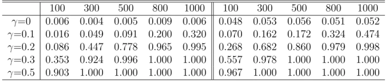
First, the uninformative weight function w(x) = 1 is considered. For Model I, the simulation result presented on the left part of Table 3.1 shows that the empirical levels are less than the nominal levels without any exception, hence the proposed tests are conservative. This is very common for nonparametric smoothing tests. The test has small powers against the alternative models for small sample sizes, but the power improves with sample sizes getting larger. 100 300 500 800 1000 100 300 500 800 1000 γ=0 0.006 0.004 0.005 0.009 0.006 0.048 0.053 0.056 0.051 0.052 γ=0.1 0.016 0.049 0.091 0.200 0.320 0.070 0.162 0.172 0.324 0.474 γ=0.2 0.086 0.447 0.778 0.965 0.995 0.268 0.682 0.860 0.979 0.998 γ=0.3 0.353 0.924 0.996 1.000 1.000 0.557 0.978 1.000 1.000 1.000 γ=0.5 0.903 1.000 1.000 1.000 1.000 0.967 1.000 1.000 1.000 1.000
Table 3.1: d=1. Empirical powers based on Model I, left panel based on normal simulation, right panel based on bootstrap
In general, bootstrap provides more accurate approximation to the distribution of the test statistic than the asymptotic normal distribution. Under the null hypothesis, the test statisticTnhas an asymptotic standard normal distribution. Therefore,Tnis asymptotically
pivotal, which enables us to conduct a parametric bootstrap. To find the parametric boot-strap critical values, for each sample size, we repeat the simulation under the null hypothesis 800 times, the critical values are then obtained by finding out the upper 97.5th percentile and lower 2.5th percentile of these 800 test statistics. Using the bootstrap critical values, we conduct the simulation again, and the empirical levels and powers are taken as the relative frequencies of how many times the test statistics being lower than the 2.5th percentile and bigger than the 97.5th percentile. The right part of Table 3.2 reports the simulation results. As expected, all the empirical levels are very close to the nominal level 0.05, and the powers are much larger than the ones reported on the left part of Table 3.1.
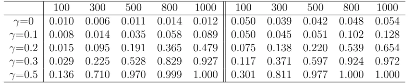
We also did a simulation study based on Model II. Under this condition, the same test statistic is used with ˆξi being replace by I(Yi = 0)−Fε(−m(Xi,θ)). The simulation resultˆ is presented in Table 3.2. The left part of Table 3.2 is the simulation results based on the critical values from Theorem 1, while the right part of Table 3.2 is the simulation results based on the bootstrap critical values. As discussed in Chapter 2, the test is much less powerful than the one based on Model I.
100 300 500 800 1000 100 300 500 800 1000 γ=0 0.010 0.006 0.011 0.014 0.012 0.050 0.039 0.042 0.048 0.054 γ=0.1 0.008 0.014 0.035 0.058 0.089 0.050 0.045 0.051 0.102 0.128 γ=0.2 0.015 0.095 0.191 0.365 0.479 0.075 0.138 0.220 0.539 0.654 γ=0.3 0.029 0.225 0.528 0.829 0.927 0.117 0.371 0.597 0.924 0.972 γ=0.5 0.136 0.710 0.970 0.999 1.000 0.301 0.811 0.977 1.000 1.000
Table 3.2: d=1. Empirical powers based on Model II, left panel based on normal simulation, right panel based on bootstrap
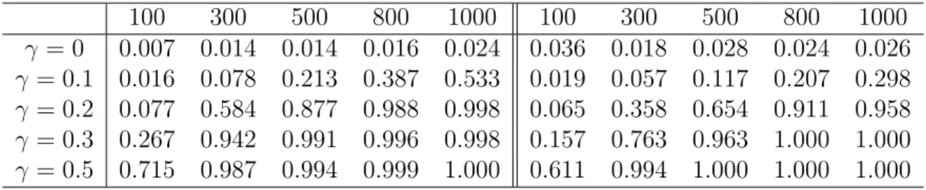
For comparison purpose, we also conduct simulation studies based on the optimal weight functions. Let z = (α +βx)/σε. For model I, the optimal weight function is w(x) = Φ(z)x2/τ2(x), andτ2(x) =σε2[1 +z2]Φ(z) +σε2zφ(z)−σε2[zΦ(z) +φ(z)]2. For model II, the optimal weight function is w(x) =φ(z)x2/τ2(x), and τ2(x) = Φ(z)(1−Φ(z)). Again, α, β and σε are estimated as above. Simulation results are presented in Table 3.3. The left part
is for the test based on model I, and the right part is for the test based on the model II. It is easily seen that the empirical levels are closer to 0.05 than the ones reported in Table 3.1 and 3.2, and as expected, the empirical powers are larger than the corresponding ones in Table 3.1 and 3.2 for large sample sizes. Recall that the optimal weight functions are indeed ”optimal” asymptotically, so it would be no surprise to us when the empirical powers are less than the ones reported in Table 3.1 and 3.2 for small sample cases. Also, the test based on the model I is more powerful than the one based on the model II.
100 300 500 800 1000 100 300 500 800 1000 γ = 0 0.007 0.014 0.014 0.016 0.024 0.036 0.018 0.028 0.024 0.026 γ = 0.1 0.016 0.078 0.213 0.387 0.533 0.019 0.057 0.117 0.207 0.298 γ = 0.2 0.077 0.584 0.877 0.988 0.998 0.065 0.358 0.654 0.911 0.958 γ = 0.3 0.267 0.942 0.991 0.996 0.998 0.157 0.763 0.963 1.000 1.000 γ = 0.5 0.715 0.987 0.994 0.999 1.000 0.611 0.994 1.000 1.000 1.000
Table 3.3: d=1. Empirical powers with optimal weights, left panel based on Model I, right panel based on Model II
Simulation 2: To see the performance of the proposed test when d >1, we generate the data from the models
Y∗ =α+β1X1+β2X2+γ(X12+X22) +ε, Y =max{Y∗,0}. (3.2) In the simulation, (X1, X2) is from a bivariate normal distribution with0 mean vector, and identity covariance matrix with ε ∼ N(0, σ2
ε). The true regression parameters are chosen to be α = β1 = β2 = σε2 = 1. We choose the product of two standard normal density functions as the kernel function, and h = n−1/7 as the bandwidth. Theoretically, under current settings,P(ε≤ −1−X1−X2)≈28% observations ofY∗ are truncated below 0 when γ = 0. The censReg function in the R package censReg is used to estimate all unknown parameters.
For Model I, the simulation result presented on the left part of Table 3.4 preserves to be conservative. The power enhances with the increase of sample size. Similar to the one-dimensional case, we conduct a parametric bootstrap simulation and the results are shown
on the right part of Table 3.4. Clearly, the nominal level 0.05 is well preserved in the bootstrap simulation and the power is much larger than the one shown on the left part of Table 3.4. 100 300 500 800 1000 100 300 500 800 1000 γ=0 0.002 0.008 0.010 0.009 0.019 0.054 0.047 0.050 0.045 0.046 γ=0.1 0.034 0.158 0.283 0.529 0.672 0.111 0.221 0.388 0.640 0.802 γ=0.2 0.247 0.838 0.985 1.000 1.000 0.423 0.903 0.994 1.000 1.000 γ=0.3 0.690 0.999 1.000 1.000 1.000 0.851 1.000 1.000 1.000 1.000 γ=0.5 0.997 1.000 1.000 1.000 1.000 1.000 1.000 1.000 1.000 1.000
Table 3.4: d=2, ρ(X1, X2) = 0.2, Empirical powers based on Model I, left panel based on normal simulation, right panel based on bootstrap
The simulation result for Model II is presented in Table 3.5. The formulation of Table 3.5 is the same as the one in Table 3.4. It is easily seen that the test is much less powerful than the one based on Model I.
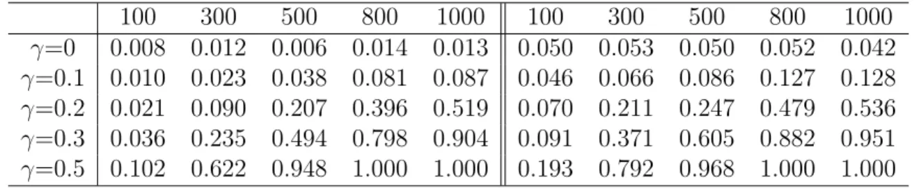
100 300 500 800 1000 100 300 500 800 1000 γ=0 0.008 0.012 0.006 0.014 0.013 0.050 0.053 0.050 0.052 0.042 γ=0.1 0.010 0.023 0.038 0.081 0.087 0.046 0.066 0.086 0.127 0.128 γ=0.2 0.021 0.090 0.207 0.396 0.519 0.070 0.211 0.247 0.479 0.536 γ=0.3 0.036 0.235 0.494 0.798 0.904 0.091 0.371 0.605 0.882 0.951 γ=0.5 0.102 0.622 0.948 1.000 1.000 0.193 0.792 0.968 1.000 1.000
Table 3.5: d=2, ρ(X1, X2) = 0.1, Empirical powers based on Model II, left panel based on normal simulation, right panel based on bootstrap
We also did some simulation studies whenX1andX2 are correlated withρ(X1, X2) = 0.2 and ρ(X1, X2) = 0.5. Table 3.6 is for the occasion when ρ(X1, X2) = 0.2. The left part of this table is the result of the simulation study based on Model I, while the other part is based on Model II.
Table 3.7 is for the occasion when ρ(X1, X2) = 0.5. The left part of this table is the result of the simulation study based on Model I, while the other part is based on Model II.
100 300 500 800 1000 100 300 500 800 1000 γ=0 0.003 0.008 0.009 0.008 0.019 0.004 0.013 0.009 0.019 0.010 γ=0.1 0.025 0.125 0.240 0.474 0.589 0.007 0.020 0.029 0.060 0.066 γ=0.2 0.219 0.786 0.978 1.000 1.000 0.016 0.074 0.140 0.309 0.423 γ=0.3 0.666 0.999 1.000 1.000 1.000 0.033 0.194 0.430 0.750 0.881 γ=0.5 0.997 1.000 1.000 1.000 1.000 0.118 0.650 0.970 1.000 1.000
Table 3.6: d=2,ρ(X1, X2) = 0.2, Empirical powers, left panel based on Model I, right panel based on Model II 100 300 500 800 1000 100 300 500 800 1000 γ=0 0.002 0.009 0.007 0.007 0.016 0.002 0.011 0.007 0.013 0.015 γ=0.1 0.025 0.097 0.202 0.425 0.535 0.007 0.020 0.035 0.053 0.053 γ=0.2 0.185 0.751 0.967 1.000 1.000 0.013 0.058 0.109 0.265 0.358 γ=0.3 0.683 0.998 1.000 1.000 1.000 0.029 0.165 0.358 0.684 0.828 γ=0.5 0.995 1.000 1.000 1.000 1.000 0.181 0.756 0.990 1.000 1.000
Table 3.7: d=2,ρ(X1, X2) = 0.5, Empirical powers, left panel based on Model I, right panel based on Model II
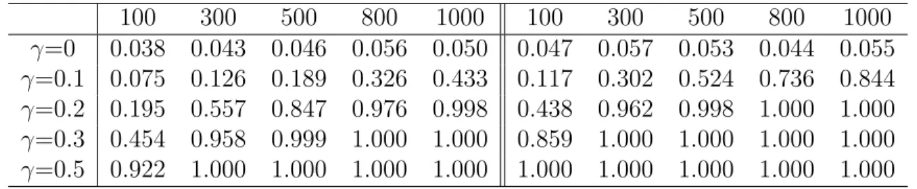
Remark 3.1: For the purpose of comparison, a simulation study for simple null hypothe-ses is conducted by using the same setups as in Simulation 1 and 2 but assuming that α=β1 =β2 =σε2 = 1 are all known in the null models. The results of the simulation under this circumstance are shown in Table 3.8. The empirical level is much closer to the nominal level 0.05 in all cases.
100 300 500 800 1000 100 300 500 800 1000 γ=0 0.038 0.043 0.046 0.056 0.050 0.047 0.057 0.053 0.044 0.055 γ=0.1 0.075 0.126 0.189 0.326 0.433 0.117 0.302 0.524 0.736 0.844 γ=0.2 0.195 0.557 0.847 0.976 0.998 0.438 0.962 0.998 1.000 1.000 γ=0.3 0.454 0.958 0.999 1.000 1.000 0.859 1.000 1.000 1.000 1.000 γ=0.5 0.922 1.000 1.000 1.000 1.000 1.000 1.000 1.000 1.000 1.000
Table 3.8: Simulation results for the simple hypotheses, left panel based on Model I, right panel based on Model II
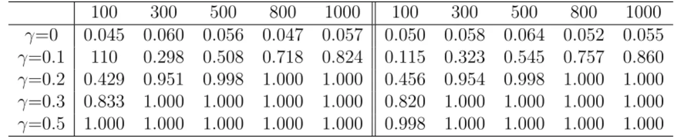
Remark 3.2 : Under the same setup as described in Remark 3.1, we also did the simula-tion when ρ(X1, X2) = 0.2 and ρ(X1, X2) = 0.5, respectively. The results of the simulation
under this circumstance are shown in Table 3.9. The empirical level is much closer to the nominal level 0.05 in all cases.
100 300 500 800 1000 100 300 500 800 1000 γ=0 0.045 0.060 0.056 0.047 0.057 0.050 0.058 0.064 0.052 0.055 γ=0.1 110 0.298 0.508 0.718 0.824 0.115 0.323 0.545 0.757 0.860 γ=0.2 0.429 0.951 0.998 1.000 1.000 0.456 0.954 0.998 1.000 1.000 γ=0.3 0.833 1.000 1.000 1.000 1.000 0.820 1.000 1.000 1.000 1.000 γ=0.5 1.000 1.000 1.000 1.000 1.000 0.998 1.000 1.000 1.000 1.000
Table 3.9: Simulation results for the simple hypotheses, left panel when ρ(X1, X2) = 0.2, right panel when ρ(X1, X2) = 0.5
Remark 3.3 : We also made a comparison study with Song and Zhang (2011)’s test pro-cedure, and the results are mixed. When we rely on R packages to estimate the parameter, for Model I, the proposed test is slightly powerful than Song and Zhang (2011)’s whend = 1, but less powerful when d= 2. The conclusion reverses if bootstrap critical values are used. Song and Zhang (2011)’s test is more powerful than the test proposed in this report. For Model II, the test proposed in this report outperforms Song and Zhang (2011)’s for both of the cases. For simple null hypothesis with α = β1 = β2 = σ2ε = 1 all known, the result of the comparison with Song and Zhang (2011)’s test doesn’t change much.
3.2
A Real Data Application
Thomas A. Mroz in 1987 undertook a systematic analysis of several theoretic and statistical assumptions used in many empirical models of female labor supply. The data for the analysis came from the University of Michigan Panel Study of Income Dynamics for the year 1975, which has been cited multiple time either for the purpose of research, or for the purpose of academic demonstration.
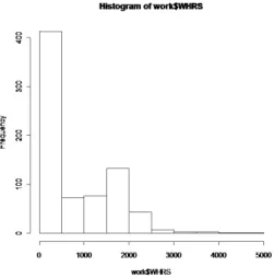
The sample consists of 753 married white women between the ages of 30 and 60 in 1975, with 428 working at some time during the year, while the remaining 325 observations are women who did not work for pay in 1975. The dependent variable, the wife’s annual hours
of work, is the product of the number of weeks the wife worked for money in 1975 and the average number of hours of work per week during the weeks she worked. The histogram of wife’s annual hours of work of Figure 1 clearly shows that a large amount of women didn’t participate in any work in the labor market, a reason why Tobit regression model is needed.
Figure 3.1: Histogram of wife’s annual hours of work
Instead of using all of the 17 variables in the original dataset, we focus on two of them, wife’s educational attainment, in years, denoted as WE, and actual years of wife’s previous labor market experience, denoted as AX.
We treat both wife’s educational attainment and previous labor market experience as independent variables to explain wife’s annual hours of work. The Tobit regression takes the form: Yi∗ = m(X) +εi =−1364 + 0.7644xW E + 0.6981xAX +εi, i= 1,2, ..., n, Yi = Yi∗ if Yi∗ >0, 0 otherwise
We apply the test proposed in this report to check if there is adequacy evidence to explain wife’s wife’s annual hours of work by using educational attainment and previous
labor market. The hypothesis is:
H0 :m(x) =m(x, θ) for some θ∈Θ, versus H1 :H0 is not true
We get 4.85 as the test statistic, the corresponding value of which is 1.239401e-06. Since p-value is less than 0.05, there is significant evidence to show the inappropriate use of the linear function. Thus, it’s not appropriate to use the linear function to express the relationship between wife’s annual hours of work and wife’s education level and previous labor market.
Chapter 4
Conclusion
We proposed a nonparametric lack-of-fit test to check the adequacy of the presumed para-metric form for the regression function in Tobit regression models by applying Zheng’s device with weighted residuals. It is shown that testing the null hypothesis for the stan-dard Tobit regression models is equivalent to testing a new null hypothesis of the classic regression models, one of which was built based on the whole data set, while the other one of which was built based on the part that has been truncated. An optimal weight function is identified to maximize the local power of the test.The proposed test statistic is shown to be asymptotically normal under null hypothesis, consistent against some fixed alternatives, and has nontrivial power for some local nonparametric power for some local nonparametric alternatives. The applicability of the test proposed is verified by the performance of the finite sample Monte-Carlo simulations.
Bibliography
[1] Amemiya, T. (1973). Regression analysis when the dependent variable is truncated normal. Econometrica, 41, 997-1016.
[2] Amemiya, T. (1984). Tobit models: A survey.J. of Econometrics, 24(1-2), 3-61. [3] Ekstrand, C.,Carpenter, T.E. (1998). Using a tobit regression model to analyse risk
factors for foot-pad dermatitis in commercially grown broilers. Preventive Veterinary Medicine, 37(1-4), 219-228
[4] Anastasopoulos, P., Tarko, A., Mannering, F., (2008). Tobit analysis of vehicle accident rates on interstate highways. Accident Analysis and Prevention 40(2), 768-775
Andrew P. Tarko, Panagiotis Ch. Anastasopoulos, Fred L. Mannering (2007). Tobit analysis of vehicle accident rates on interstate highways. Accident Analysis and Pre-vention, 40(2008)768-775
[5] Goldberger, A.S. (1964).Econometric theory. Wiley, New York.
[6] Hall, P. J. (1984). Central limit theorem for integrated square error of multivariate nonparametric density estimators. J. Multivariate Anal., 14(1), 1-16
[7] H¨ardle, W., Mammen, E. (1993). Comparing nonparametric versus parametric regres-sion fits. Ann, Statist., 21(4), 1926-1947
[8] Heckman, J. J. (1976). The common structure of statistical models of truncation, sam-ple selection, and limited dependent variables and a simsam-ple estimator for such models. Ann. Econom. Social Meas., 5(4), 475-492
[9] Heckman, J. J. (1979). Sample selection bias as a specification error. Econometrica, 47(1),153-162
[10] Horowitz, J. L., Neumann, G. R. (1989). Specification testing in censored regression models: parametric and semiparametric methods. J. Appl. Econometrics, 4, supple-ment issue, 61-86.
[11] Jennrich, R. I. (1969). Asymptotic properties of non-linear least squares estimators. Ann. Math. Statist., 40(2),633-643.
[12] Koul, Hira L., Ni, P. (2004). Minimum distance regression model checking, J. Stat. Plann. Inference, 119(1), 109-141.
[13] Lee, L. F. (1981). A specification test for normality assumption for the truncated and censored tobit models. Discussion paper 44, Center for Econometrics and decision sci-ences, University of Florida.
[14] Lewbel, A. and Linton, O. B. (2002). Nonparametric censored and truncated regression. Econometrica, 70,765-779.
[15] Lichtenberg, E., Shapiro, L. K. (1997). Agriculture and nitrate concentration in Mary-land community water system wells. J. Environ. Qual., 26(1), 145-153.
[16] Lin, T. F. and Schmidt, P. (1984). A test of the tobit specification against an alternative suggested by Cragg. The Review of Economics and Statistics, 66(1), 174-177.
[17] McConnel, C. E., Zetzman, M. R. (1993). Urban/rural differences in health service utilization by elderly persons in the United States. J. Rural Health, 9(4), 270-280. [18] Nelson, F. D. (1981). A test for misspecification in the censored normal model.
Econo-metrica, 49(5), 1317-1330.
[19] Olsen, R. J. (1980). Approximating a truncated normal regression with the method of moments. Econometrica, 48(5), 1099-1106.
[20] Powell, J. L. (1984). Least abosulte deviations estimation for the censored regression model. J. Econometrics, 25(3),303-325.
[21] Song, W. X. (2011). Distribution-free test in Toibt mean regression model. J. Stat. Plann. Inference, 141(8), 2891-2901.
[22] Song, W. X. (2011). Empirical L2-Distance Lack-of-Fit Tests For Tobit Regression Models. Submitted to JMVA.
[23] Tobin, J. (1958). Estimation of Relationships for Limited Dependent Variables. Econo-metrica, 26(1), 24-36.
[24] Thomas A.Mroz (1987) The Sensitivity of an Empirical Model of Married Women’s Hours of Work to Economic and Statistical Assumptions. Econometrica, 765-799. [25] Wang, L. (2007). A simple nonparametric test for diagnosing nonlinearity in Tobit
median regression model. Stat. and Prob. Letters, 77(10), 1034-1042.
[26] White, H. (1981). Consequences and detection of misspecified nonlinear models. JASA, 76(374), 419-433.
[27] White, H. (1982). Maximum likelihood estimation of misspecified models. Economet-rics, 50(1), 1-25.
[28] Zheng, J. X. (1996). A consistent test of functional form via nonparametric estimation techniques. J. Econometrics, 75(2), 263-289.
[29] Zhou, X. B. (2007). Semiparametric and Nonparametric Estimation of Toibt Models. PhD thesis, Department of Economics, Hong Kong University of Science and Technol-ogy.
Appendix A
R-Programs
The first part of our simulation is on Tobit linear regression with one predictor, composite hypothesis. Note that this is the code when the σε is unknown and estimated, but we also did simulations when σε is known.
library(VGAM) set.seed(987654) table1=matrix(c(1:25),nrow=5,ncol=5) colnames(table1)<-c("n=100","n=300","n=500","n=800","n=1000") rownames(table1)<-c("m0=0","m1=0.1","m2=0.2","m3=0.3","m4=0.5") m<-c(100,300,500,800,1000) r<-c(0,0.1,0.2,0.3,0.5) for (j in 1:length(m)){ for (k in 1:length(r)){ freq=0; for(i in seq(1000)) { # Generating Data n=m[j] sx=1
se=1 a=1 b=1 x=rnorm(n,0,sx) e=rnorm(n,0,se) ystar=a+b*x+r[k]*x^2+e y=pmax(ystar,0)
# Estimation of regression parameters fit=vglm(y~x, tobit(Lower=0, Upper=Inf)) a=fit@coefficients[1] b=fit@coefficients[3] sig=exp(fit@coefficients[2]) # Test Statistics res=y-((a+b*x)*pnorm((a+b*x)/sig)+dnorm((a+b*x)/sig)*sig) res2=res^2 res4=res^4 h=n^(-1/5) K=function(u){dnorm(u)} xdif=kronecker(x,x,"-") A1=matrix(K(xdif/h)/h,nrow=n) A2=matrix((K(xdif/h))^2/h,nrow=n) Vn=(t(res)%*%A1%*%res-sum(diag(A1)*res2))/(n*(n-1)) Sn=2*(t(res2)%*%A2%*%res2-sum(diag(A2)*res4))/(n*(n-1)) Tn=n*sqrt(h)*Vn/sqrt(Sn) freq=freq+(abs(Tn)>=1.96)
}
table1[k,j]=freq/1000 }
} table1
The second part of our simulation is on Tobit linear regression with two predictors. Note that this is the code when the two predictors are independent. We also did simulations when the two predictors are not independent.
library(VGAM) library(maxLik) library(miscTools) library(censReg) library(mvtnorm) set.seed(98765432) table1=matrix(c(1:25),nrow=5,ncol=5) colnames(table1)<-c("n=100","n=300","n=500","n=800","n=1000") rownames(table1)<-c("m0=0","m1=0.1","m2=0.2","m3=0.3","m4=0.5") m<-c(100,300,500,800,1000) r<-c(0,0.1,0.2,0.3,0.5) for (j in 1:length(m)){ for (k in 1:length(r)){ freq=0; for(i in seq(1000)) { #Generating Data
n=m[j] sx=matrix(c(1,0,0,1),2) se=1 a=1 b1=1 b2=1 xno=rmvnorm(n,mean=c(0,0),sx) x1=xno[ ,1] x2=xno[ ,2] e=rnorm(n,0,se) ystar=a+b1*x1+b2*x2+r[k]*(x1^2+x2^2)+e y=pmax(ystar,0) data=data.frame(cbind(y,x1,x2))
#Estimation of regression parameters
estimation <- censReg( y ~ x1 + x2, data = data ) a=summary(estimation)$estimate[1] b1=summary(estimation)$estimate[2] b2=summary(estimation)$estimate[3] sigma=exp(summary(estimation)$estimate[4]) #Test Statistics res=y-((a+b1*x1+b2*x2)*pnorm((a+b1*x1+b2*x2)/sigma)+dnorm((a+b1*x1+b2*x2)/sigma)*sigma) res2=res^2 res4=res^4 h=n^(-1/7) K=function(u,v){dnorm(u)*dnorm(v)}
x1dif=kronecker(x1,rep(1,n))-kronecker(rep(1,n),x1) x2dif=kronecker(x2,rep(1,n))-kronecker(rep(1,n),x2) A1=matrix(K(x1dif/h,x2dif/h)/h^2,nrow=n) A2=matrix((K(x1dif/h,x2dif/h))^2/h^2,nrow=n) Vn=(t(res)%*%A1%*%res-sum(diag(A1)*res2))/(n*(n-1)) Sn=2*(t(res2)%*%A2%*%res2-sum(diag(A2)*res4))/(n*(n-1)) Tn=n*h*Vn/sqrt(Sn) freq=freq+(abs(Tn)>=1.96) } table1[k,j]=freq/1000 } } table1
The last part of our simulations is Tobit linear regression, simple hypotheses. The codes below are the one predictor case and the two predictor case.
(a) One Predictor Case:
library(VGAM) set.seed(987654) table1=matrix(c(1:25),nrow=5,ncol=5) colnames(table1)<-c("n=100","n=300","n=500","n=800","n=1000") rownames(table1)<-c("m0=0","m1=0.1","m2=0.2","m3=0.3","m4=0.5") m<-c(100,300,500,800,1000) r<-c(0,0.1,0.2,0.3,0.5) for (j in 1:length(m)){ for (k in 1:length(r)){ freq=0;
for(i in seq(1000)) { # Generating Data n=m[j] sx=1 se=1 a=1 b=1 x=rnorm(n,0,sx) e=rnorm(n,0,se) ystar=a+b*x+r[k]*x^2+e y=pmax(ystar,0) # Test Statistics res=y-((a+b*x)*pnorm((a+b*x)/se)+dnorm((a+b*x)/se)*se) res2=res^2 res4=res^4 h=n^(-1/5) K=function(u){dnorm(u)} xdif=kronecker(x,x,"-") A1=matrix(K(xdif/h)/h,nrow=n) A2=matrix((K(xdif/h))^2/h,nrow=n) Vn=(t(res)%*%A1%*%res-sum(diag(A1)*res2))/(n*(n-1)) Sn=2*(t(res2)%*%A2%*%res2-sum(diag(A2)*res4))/(n*(n-1)) Tn=n*sqrt(h)*Vn/sqrt(Sn) freq=freq+(abs(Tn)>=1.96)
}
table1[k,j]=freq/1000 }
} table1
(b)Two Predictor Case:
library(VGAM) library(maxLik) library(miscTools) library(censReg) library(mvtnorm) set.seed(987654) table1=matrix(c(1:25),nrow=5,ncol=5) colnames(table1)<-c("n=100","n=300","n=500","n=800","n=1000") rownames(table1)<-c("m0=0","m1=0.1","m2=0.2","m3=0.3","m4=0.5") m<-c(100,300,500,800,1000) r<-c(0,0.1,0.2,0.3,0.5) for (j in 1:length(m)){ for (k in 1:length(r)){ freq=0; for(i in seq(1000)) { # Generating Data n=m[j] sx=matrix(c(1,0,0,1),2) se=1
a=1 b1=1 b2=1 xno=rmvnorm(n,mean=c(0,0),sx) x1=xno[ ,1] x2=xno[ ,2] e=rnorm(n,0,se) ystar=a+b1*x1+b2*x2+r[k]*(x1^2+x2^2)+e y=pmax(ystar,0) #Test Statistics res=y-((a+b1*x1+b2*x2)*pnorm((a+b1*x1+b2*x2)/se)+dnorm((a+b1*x1+b2*x2)/se)*se) res2=res^2 res4=res^4 h=n^(-1/7) K=function(u,v){dnorm(u)*dnorm(v)} x1dif=kronecker(x1,rep(1,n))-kronecker(rep(1,n),x1) x2dif=kronecker(x2,rep(1,n))-kronecker(rep(1,n),x2) A1=matrix(K(x1dif/h,x2dif/h)/h^2,nrow=n) A2=matrix((K(x1dif/h,x2dif/h))^2/h^2,nrow=n) Vn=(t(res)%*%A1%*%res-sum(diag(A1)*res2))/(n*(n-1)) Sn=2*(t(res2)%*%A2%*%res2-sum(diag(A2)*res4))/(n*(n-1)) Tn=n*h*Vn/sqrt(Sn) freq=freq+(abs(Tn)>=1.96) } table1[k,j]=freq/1000 }
} table1