Optimization and Performance Study of Select Heating Ventilation and Air Conditioning Technologies for Commercial Buildings

(1)

University of South Florida

Scholar Commons

Graduate Theses and Dissertations

Graduate School

3-30-2017

Optimization and Performance Study of Select

Heating Ventilation and Air Conditioning

Technologies for Commercial Buildings

Rajeev Kamal

University of South Florida, [email protected]

Follow this and additional works at:

http://scholarcommons.usf.edu/etd

Part of the

Engineering Commons, and the

Oil, Gas, and Energy Commons

This Dissertation is brought to you for free and open access by the Graduate School at Scholar Commons. It has been accepted for inclusion in Graduate Theses and Dissertations by an authorized administrator of Scholar Commons. For more information, please contact

[email protected].

Scholar Commons Citation

Kamal, Rajeev, "Optimization and Performance Study of Select Heating Ventilation and Air Conditioning Technologies for

Commercial Buildings" (2017).Graduate Theses and Dissertations.

(2)

Optimization and Performance Study of Select Heating Ventilation and Air Conditioning Technologies for Commercial Buildings

by

Rajeev Kamal

A dissertation submitted in partial fulfillment of the requirements for the degree of

Doctor of Philosophy

Department of Chemical and Biomedical Engineering College of Engineering

University of South Florida

Major Professor: D. Yogi Goswami, Ph.D. Elias Stefanakos, Ph.D. Babu Joseph, Ph.D. Tapas Das, Ph.D. Herbert A. Ingley, Ph.D. Date of Approval: March 2, 2017

(3)

Dedication

(4)

Acknowledgments

I express my sincere gratitude to Dr. D. Yogi Goswami, my advisor, for his support, constructive guidance and advice throughout my research and this dissertation. His knowledge and reputation in the academic and research community allowed me to obtain necessary funding and opportunity to conduct this research.

I would also like to extend my gratitude to my doctoral committee, Dr. Elias Stefanakos for his mentorship and encouragement, Dr. Babu Joseph and Dr. Tapas Das for helping me bring this work to a practical industry acceptance and especially for Dr. Herbert A. Ingley for his training and inputs from his experience in HVAC field. Special thanks to the staff at Clean Energy Research Center (CERC) Barbara Graham, Dr. Chand Jotshi, Charles Garretson, and David Goslin who helped me from time to time in conducting this research and during my tenure at the University of South Florida.

I am thankful to my friends and colleagues at the CERC lab who have been helpful throughout my research through their personal support and professional contributions, Chatura Wickramaratne, Arun Kumar Narasimhan, Francesca Moloney, Abhinav Bhardwaj, and Saumya Sharma.

(5)

Table of Contents

List of Tables iv

List of Figures vi

Abstract x

Chapter 1 Introduction 1

1.1 Energy Consumption in Buildings 2

1.1.1 HVAC in Buildings 2

1.2 Challenges for Power Utilities 3

1.3 Theoretical Background 5

1.3.1 Heating Ventilation and Air Conditioning in Commercial Buildings 5

1.3.2 Heat Pumps 5

1.3.3 Working Principle of Heat Pumps 6

1.4 Heat Pump Technology 7

1.4.1 Vapor Compression Heat Pump 7

1.4.2 Absorption Systems 8

1.4.3 Heat Pump Heat Sources 10

1.4.4 Classification 10

1.5 Gas Engine-driven Heat Pump 10

1.5.1 Description of GEHPs 11

1.6 Thermal Energy Storage for Cooling/Heating 12

1.6.1 Benefits to Consumer 14

1.6.2 Benefits to Utilities 15

Chapter 2 Research Objectives 17

Chapter 3 Performance Study of GEHPs 19

3.1 Field Setup and Measurement Devices 19

3.1.1 Instrumentation 20

3.1.2 Installation of Data Aquisition System 23

3.1.3 LabView Program 24

3.2 Data Collection 25

3.3 Data Processing and Synchronization 26

3.4 Analysis 27

3.5 Uncertainty in COP Calculation 30

3.6 Field Operation and Performance Results 31

3.7 Measured Performance 34

3.8 Comparison with Laboratory and Other Field Experiments 35

(6)

3.10 Economic Analysis 40

3.11 Performance of GEHP vs. EHP 41

3.11.1 DeBary Building Model 41

3.11.2 Economic Analysis 43

3.12 Performance Prediction at Okaloosa, FL and Plant City, FL 44

3.13 Summary and Discussion 45

Chapter 4 Integration of Cooling Thermal Energy Storage in Commercial Buildings 47

4.1 Benefits of Adopting Thermal Energy Storage 47

4.1.1 Benefits to Power Generators 47

4.1.2 Thermal Energy Storage for Air-conditioning 48

4.2 Research Methodology - Thermal Energy Storage for Peak Reduction 49

4.2.1 Location and Case 49

4.3 Building Energy Modeling 50

4.3.1 Building Information Model for Reference Building 51

4.3.2 Model Operation Requirements 54

4.3.3 Cost Minimization 55

4.3.4 Control Requirements 56

4.4 Modified Plant Loop Description 56

4.4.1 Control Strategy 59

4.4.2 System Sizing for Demand Side Management 60

4.5 Performance with New Configuration 61

4.6 Optimization of the System Size for Storage 62

4.6.1 Ice Storage Model Optimization 63

4.6.2 System Optimization for Chilled Water Mixed and Stratified Tank Storage 64

4.7 Results After System Optimization 65

4.8 Economic Comparison and Discussion: Optimal TES System for Commercial Buildings 68

Chapter 5 Impact of Adopting Thermal Energy Storage in Buildings 71

5.1 Tampa Utility Generation and Demand Analysis 71

5.1.1 Benefits of Peak Demand Shifting from Commercial Buildings 72

5.2 TES Adoption Impact on Regional Demand Profile 74

5.3 Benefits of Storage to Power Grid and Renewable Energy Systems 78

5.3.1 Energy Storage Applications 80

5.3.2 Thermal Energy Storage Value for Grid 80

5.3.3 Renewable Generation from Solar 80

Chapter 6 Conclusion 83

6.1 Summary 83

6.2 Conclusions and Recommendations 84

List of References 87

Appendix A Abbreviations 94

(7)

Appendix C Supporting Information for Chapter 3 96

C.1 Data Collection of Operating Parameters 97

C.2 Procedure of Processing Collected Data from GEHP Data Logger 100

C.3 Power Query Code for Data Compilation 119

Appendix D Optimization Results - JEPlus 120

(8)

List of Tables

Table 1. Specifications of GEHP systems at the field 20

Table 2. Measurements sensors accuracy 22

Table 3. June performance of GEHP units 34

Table 4. July performance of GEHP units 34

Table 5. August performance of GEHP units 34

Table 6. September performance of GEHP units 35

Table 7. Engine specification 37

Table 8. Performance variation of GEHP3 for engine RPM range of 1000 to 1950 38

Table 9. Maximum load operation performance 39

Table 10. Case for maximum possible average COPunit 40

Table 11. Building characteristics for EnergyPlus model 52

Table 12. GSDT consumer electricity rates for Tampa, FL 56

Table 13. Tactical control functions 60

Table 14. Annual simulation results of optimized configuration 65

Table 15. Commercial building share based on activity 74

Table C.1. Specification of sensors installed at DeBary, FL 96

Table C.2. Validation of correct source files 101

Table C.3. Measured performance data for 4 GEHP units 104

Table C.4. Running costs calculated for the DeBary four GEHP units 105

(9)

Table C.6. Model results EER-11.8 EHP system 108

Table C.9. Model results for Okaloosa, FL 114

Table C.10. Model results for Plant City, FL 116

(10)

List of Figures

Figure 1. World petroleum and liquid fuel consumption by end-use sector 2010 [3] 1

Figure 2. Building energy consumption outlook-US Energy Information Administration 2

Figure 3. Buildings primary energy end-use in the US (2010) 3

Figure 4. ‘The Duck Curve’ - California ISO’s prediction of the demand-supply gaps till 2020 [6] 4

Figure 5. Operation of heat pump and heat engine between two temperature levels 6

Figure 6. Schematic of a vapor compression heat pump [15] 8

Figure 7. Schematic of an absorption heat pump 9

Figure 8. Working principle of a GEHP 12

Figure 9. Useful work lost from the fuel source to cooling end use [23] 12

Figure 10. Office building of Florida Public Utilities, Debary, FL 19

Figure 11. GEHP and AHU configuration at the site 20

Figure 12. Remote data logging system 21

Figure 13. 8-ton units housing condenser and gas-engine 21

Figure 14. Field instrumentation for remote data collection 21

Figure 15. Location of the sensors in the GEHP unit 22

Figure 16. Krohne 1000 coriolis meter with MFC 300 converter 23

Figure 17. IMAC system pulser attached to the natural gas flow meter 23

Figure 18. Dwyer temperature and humidity sensor 23

Figure 19. cDAQ-9138 data acquisition system 23

(11)

Figure 21. Wattmeters for the outdoor units 23

Figure 22. Wattmeters for the AHU's 24

Figure 23. Data logging system 24

Figure 24. Refrigerant flow meters wired and connected to the DAQ system 24

Figure 25. DAQ logging installation inside the warehouse 24

Figure 26. Post-installation setup 25

Figure 27. Schema of USF database 27

Figure 28. Source and host database communication setup for USF server 27

Figure 29. Monthly natural gas consumption by the four gas heat pumps 29

Figure 30. Electricity use by the GEHP1 indoor and outdoor units for the month of August-2014 30

Figure 31. Field performance during summer 32

Figure 32. Cooling delivered and energy use for a typical summer day 32

Figure 33. The performance of the GEHP on a typical summer day 33

Figure 34. Effect of ambient temperature on the COP achieved at 1950 RPM 33

Figure 35. Monthly average unit COP of the four GEHP units 35

Figure 36. Measured performance compared with other studies 36

Figure 37. Efficiencies inside a gas heat pump 38

Figure 38. Brake thermal efficiencies of spark ignition and compression ignition engines 38

Figure 39. Engine efficiency at full load on 1st_July-2014 ₃₉

Figure 40. Model developed for study building 42

Figure 41. Seven thermal zones air-conditioned by four GEHP units 43

Figure 42. Cost comparison of actual vs. modeled systems 44

Figure 43. Operating costs ($) of similar systems and loads as DeBary for Okaloosa and Plant City 45

(12)

Figure 45. Study components for TES use for building 50

Figure 46. DOE reference large office building 52

Figure 47. Occupancy definition for the building 53

Figure 48. Annual cooling electricity 53

Figure 49. Typical daily cooling electricity demand in a building during summer and winter 54

Figure 50. Chilled water cooling loop 54

Figure 51. Two-season peak pricing window for Tampa 55

Figure 52. Ice storage loop configuration 57

Figure 53. Chilled water storage loop configuration 58

Figure 54. Control strategy algorithm 61

Figure 55. Charging and discharging heat transfer 62

Figure 56. Optimization result: annual cost vs. annual cooling electricity 64

Figure 57. Optimization result: average part load ratio vs. annual electricity 64

Figure 58. Chiller power after optimizing the three models 66

Figure 59. Pumping power after optimizing the storage models 66

Figure 60. Chiller part load ratios after optimizing the storage models 67

Figure 61. Week operation in winter (8-15th_January) ₆₇

Figure 62. Week operation peak summer (30th_{July – 6}th_August) ₆₈

Figure 63. Reduction in annual cost of electricity after optimizing 69

Figure 64. Annual electricity use from three models for selected locations 70

Figure 65. Annual cost of electricity use from three models for selected locations 70

Figure 66. Generation capacity utilization in summer-2013, Tampa 71

Figure 67. Utility load profile for January-2013 72

(13)

Figure 69. Electricity consumption by end-use in all buildings in South Atlantic Region, 2012, US-EIA 73

Figure 70. Aggregate building electricity demand on 13th_{August-2013, Tampa, FL} ₇₅

Figure 71. Building full peak shifting scenario 76

Figure 72. Partial control- 50% peak shifting scenario 77

Figure 73. Load levelling scenario 77

Figure 74. All scenarios of peak load shifting in buildings 78

Figure 75. Variability in solar generation in four locations 81

Figure 76. Variability in wind generation in four locations 81

Figure C.1. Parameters recorded by GEHP data logger 97

Figure C.2. LabVIEW code front-end at the logging system 98

Figure C.3. LabVIEW back-end program logic 99

Figure C.4. Procedure for processing GEHP data files 100

Figure C.5. PowerQuery used for merging the individual data file to daily data files 103

Figure D.1. System optimization results for ice storage model 120

Figure D.2. System optimization results for chilled water mixed tank storage model 122 Figure D.3. System optimization results for chilled water stratified tank storage model 124

(14)

Abstract

Buildings contribute a significant part to the electricity demand profile and peak demand for the electrical utilities. The addition of renewable energy generation adds additional variability and uncertainty to the power system. Demand side management in the buildings can help improve the demand profile for the utilities by shifting some of the demand from peak to off-peak times.

Heating, ventilation and air-conditioning contribute around 45% to the overall demand of a building. This research studies two strategies for reducing the peak as well as shifting some demand from peak to off-peak periods in commercial buildings:

1. Use of gas heat pumps in place of electric heat pumps, and

2. Shifting demand for air conditioning from peak to off-peak by thermal energy storage in chilled water and ice.

The first part of this study evaluates the field performance of gas engine-driven heat pumps (GEHP) tested in a commercial building in Florida. Four GEHP units of 8 Tons of Refrigeration (TR) capacity each providing air-conditioning to seven thermal zones in a commercial building, were instrumented for measuring their performance. The operation of these GEHPs was recorded for ten months, analyzed and compared with prior results reported in the literature. The instantaneous COPunit of these systems varied

from 0.1 to 1.4 during typical summer week operation. The COP was low because the gas engines for the heat pumps were being used for loads that were much lower than design capacity which resulted in much lower efficiencies than expected.

The performance of equivalent electric heat pump was simulated from a building energy model developed to mimic the measured building loads. An economic comparison of GEHPs and conventional

(15)

electrical heat pumps was done based on the measured and simulated results. The average performance of the GEHP units was estimated to lie between those of EER-9.2 and EER-11.8 systems. The performance of GEHP systems suffers due to lower efficiency at part load operation. The study highlighted the need for optimum system sizing for GEHP/HVAC systems to meet the building load to obtain better performance in buildings.

The second part of this study focusses on using chilled water or ice as thermal energy storage for shifting the air conditioning load from peak to off-peak in a commercial building. Thermal energy storage can play a very important role in providing demand-side management for diversifying the utility demand from buildings. Model of a large commercial office building is developed with thermal storage for cooling for peak power shifting. Three variations of the model were developed and analyzed for their performance with 1) ice storage, 2) chilled water storage with mixed storage tank and 3) chilled water storage with stratified tank, using EnergyPlus 8.5 software developed by the US Department of Energy. Operation strategy with tactical control to incorporate peak power schedule was developed using energy management system (EMS). The modeled HVAC system was optimized for minimum cost with the optimal storage capacity and chiller size using JEPlus.

Based on the simulation, an optimal storage capacity of 40-45 GJ was estimated for the large office building model along with 40% smaller chiller capacity resulting in higher chiller part-load performance. Additionally, the auxiliary system like pump and condenser were also optimized to smaller capacities and thus resulting in less power demand during operation. The overall annual saving potential was found in the range of 7-10% for cooling electricity use resulting in 10-17% reduction in costs to the consumer. A possible annual peak shifting of 25-78% was found from the simulation results after comparing with the reference models. Adopting TES in commercial buildings and achieving 25% peak shifting could result in a reduction in peak summer demand of 1398 MW in Tampa.

(16)

Chapter 1 Introduction

Energy is a critical driver for the economic development of the society. There has been a continuous rise in the demand for energy over the last few decades. From 1993 to 2011, the total electricity production increased by 76% whereas the world’s population increased by 27% [1]. Despite such increase in electricity production, about 1.3 billion people are still without access to electricity [2].

Figure 1. World petroleum and liquid fuel consumption by end-use sector 2010 [3]

Most of the countries rely mostly on fossil fuels for generation of power to serve their industrial, commercial, and residential energy requirements. In 2010, the world petroleum and liquid fuel consumption were 52.3 TWh of which the transportation sector was 55% followed by the industrial sector at 32% and remaining 13% for electricity, residential and commercial sectors (Figure 1). Use of fossil fuels is a significant reason behind increasing global warming. CO2 emissions have increased by 44% globally,

which makes it imperative to use various renewable energy resources and improve the efficiency of current technologies [1]. Residential 5% _Commercial 3% Industrial 32% Transportation 55% Electricity 5% Residential Commercial Industrial Transportation Electricity

(17)

1.1 Energy Consumption in Buildings

In 2010, building energy needs accounted for 23.7 TWh of the world delivered energy demand. It is projected to grow at a rate of 1.6 % per year to 38.4 TWh by 2040. The growth of energy consumption is projected to be maximum in residential sectors in developing nations (Figure 2) [4].

Figure 2. Building energy consumption outlook-US Energy Information Administration

Buildings typically are classified as single or multi-family residential and commercial buildings, of which commercial buildings comprise offices, stores, restaurants, warehouses, government buildings and other buildings used for commercial purposes. In the US, the buildings sector accounted for about 41% of the primary energy consumption in 2010, which included space heating, cooling, and lighting as the dominant end-uses [5].

1.1.1 HVAC in Buildings

Heating Ventilation and Air-Conditioning (HVAC) and refrigeration in the US accounted for 47.9% of the total primary energy consumption in buildings in 2010. This energy demand was predicted to fall to 43.7% by 2015 due to improvements in efficiency and upgrade of the existing HVAC technology [5]. Building energy demand varies according to the type of activities, occupancy and weather conditions.

0 10 20 30 40 50 60 2010 2015 2020 2025 2030 2035 2040 De liv ere d E n ergy (q u ad rilli o n Bt u )

(18)

Heat pump (HP) is considered to be a mature technology among the commercial HVAC technologies, and it is found that the residential HVAC market is moving more towards heat pumps instead of furnaces [5]. The estimated industrial energy demand for heat consumption in Europe for 2009 was 12.3 TWh, whereas, in the residential sector it was 18.7 TWh for heating and 4.3 TWh for cooling. In addition, the estimated energy usage in the service sector was 6.1 TWh for heating and 1.7 TWh for cooling. In the US, buildings alone had primary energy end-usage of 11.8 TWh out of which the HVAC&R totaled 5.6 TWh in 2010 (Figure 3). In the US, the aggregated energy expenditure in buildings is projected to rise from $108.6 Billion (1980) to $225 Billion by 2035 (USD 2010) [5].

Figure 3. Buildings primary energy end-use in the US (2010) 1.2 Challenges for Power Utilities

All possible sources of power are usually exploited to meet the requirements during peak power demands. The cost of electricity for conventional plants is higher during peak hours due to lower efficiencies and higher fuel costs. It can be challenging to match the ever-changing demand of cities and regions while relying on just baseload conventional fossil-based power plants. With the diurnal and nocturnal variations of the energy demand, it becomes difficult for base load power plants to ramp up

Space Heating 22% Space Cooling 15% Ventilation 4% Refrigeration 6% Lighting 14% Water Heating 9% Electronics 6% Computers 3% Cooking 3% Wet Cleaning 3% Other 9% Adjust to SEDS 6% Space Heating Space Cooling Ventilation Refrigeration Lighting Water Heating Electronics Computers Cooking Wet Cleaning Other Adjust to SEDS

(19)

and down within a short duration. Use of peaking power plants during such intervals is the only feasible option for the power utilities, and this option is linked to lower efficiencies and high fuel costs [6].

Power utilities must incorporate peak power costs in their tariff to recover the investments and to run their business profitably. For the purpose of billing the consumers based on their usage, many utilities have adopted ‘time of day’ (TOD) billing that includes different tariffs during different time slots. Being able to meet peak demand, remains a challenge for the power utilities, though TOD billing provides economic viability to the utilities [7]. During peak power demands, the base-load power plants are not able to ramp-up or down to match the immediate changes in power demand. The gaps between peak and off-peak power will keep increasing unless the demand-side energy profile is managed. Figure 4 represents the widely known as ‘The Duck Curve’ of California Independent System Operator (ISO). This clearly shows that the base load generators experience a sharp dip in demand during the day, and the utilities have to address the increased ramp needed to match the energy demand during evenings [6]. Such ramp rates are a technical challenge for the present baseload power generation plants.

Figure 4. ‘The Duck Curve’ - California ISO’s prediction of the demand-supply gaps till 2020 [6] Utilities across the world focus on adopting different measures to address such present and future challenges. The gap can be addressed either by adopting (i) supply-side approach or (ii) load-modifier

(20)

approach. In the supply-side approach, the generation capacity is increased continuously until the demand-supply gap is bridged or implementing large energy storage for power plants[8]. On the other hand, the load-modifier approach involves changing the demand patterns, increasing efficiencies, and implementing distributed storage.

Since a majority of this demand is attributed to HVAC in buildings, the demand-side-management strategies for HVAC become inevitable to address such a critical issue for future buildings. This study focusses on solutions for demand shaping using two methods: i) alternative HVAC technologies such as Gas heat pumps and ii) adoption of Thermal Energy Storage for air-conditioning. Gas heat pumps use natural gas or biogas to generate the necessary compression work. Alternatively, thermal energy storage can shift electricity demand for cooling and heating thus reducing the peaks and troughs of the energy demand [9].

1.3 Theoretical Background

1.3.1Heating Ventilation and Air Conditioning in Commercial Buildings

The need for reliable and economical cooling/heating technologies is ever increasing globally. We realize how humanity will continue to seek higher levels of comfort at their place of work, residence, and commute despite the growing concerns of global environmental impact and related issues. However, the need for more efficient ways to achieve cooling/heating has been a research focus throughout the HVAC& R industry. Industry research focuses mainly on (1) improvement in equipment performance and efficiency, (2) alternative energy sources to power the system and (3) hybrid/combined applications to maximize the useful output by integrating with other technologies.

1.3.2 Heat Pumps

In 1852, the British physicist William Thomson (Lord Kelvin) described the working principle of “pumping” heat with a thermodynamic cycle for the first time [1852]. In 1856-57, Peter Ritter von Rittinger introduced first “heat pump” of 14 kW in Ebensee/Austria for salt production [1855].

(21)

Most widely used heat pumps (HP) work on either vapor compression or vapor absorption cycle. The history of vapor compression cycle goes back to 1834 with the first commercialized system made in 1850. Heat pumps are used for both heating and cooling across the globe all year round. Commercial production of HP’s in the United States began in the 1930’s, and they became very popular by 1970’s as their costs came down significantly. By 1984 about 30% of all the new buildings, both residential and commercial were using HP’s [10]. The industrial sector also started to use these technologies for drying agricultural products, and dehumidification [11]–[13]. In Europe, about 4,50,000 electrical heat pumps were installed in the year 2008 [14].

1.3.3Working Principle of Heat Pumps

A Heat Pump is based on a thermodynamic cycle that transports heat from lower temperature source to higher temperature sink. A heat pump works as a reverse heat engine by utilizing work ‘W’ to extract heat ‘Q1’ from a lower temperature heat source at ‘T1’ and deliver ‘Q2’ to a higher temperature sink at ‘T2’ and thereby creating a cooling effect as shown in Figure 5.

Figure 5. Operation of heat pump and heat engine between two temperature levels

The Coefficient of Performance (COP) is the performance indicator of a heat pump and is calculated as:

(22)

Primary Energy Ratio (PER) is used as a performance indicator in the case of engines and thermally driven heat pumps. For electrically driven heat pumps this PER can be defined as the product of the COP and the power generation efficiency of the engine that provides the work.

An ideal Carnot cycle operating between the temperatures T1 and T2 has the maximum COP, which is given as:

𝐶𝑂𝑃𝐶 =

𝑇2

𝑇2− 𝑇1

Real heat pumps cannot work ideally as a reversible cycle due to the presence of losses and limitations of real working fluids. Hence, the COPC is used as a reference for the maximum possible limit

of performance for real systems. The ratio of the real COP and COPC is defined a Carnot efficiency ηc, which

varies between 0.3 to 0.5 for small electric heat pumps and 0.5 to 0.7 for large highly efficient electric heat pumps [15].

1.4 Heat Pump Technology

Most commonly used commercial heat pump technologies are (i) the vapor compression heat pumps that use mechanical energy to drive a vapor compression cycle and (II) the absorption heat pumps that use thermal energy to drive a thermodynamic cycle to create the desired effect. Theoretically, many other thermodynamic cycle and processes can be used for heat pumps, i.e., Sterling cycle, Vuilleumier cycles, single-phase cycles (air or CO2 gas), adsorption systems, solid-vapor sorption systems, hybrid

systems, electromagnetic and acoustic processes. Heat pumps are making way into many sectors due to their advantages of efficiencies and dual conditioning (heating/cooling). Heat pumps are being researched even for mobile applications like vehicles [16]. Many of these technologies have not matured as commercially viable options, with some of them being in their early stage of development [17].

1.4.1Vapor Compression Heat Pump

A vapor compression cycle uses volatile liquids that have a lower evaporating temperature to generate cooling exploiting the properties of these fluids at different temperatures and pressures. A

(23)

compressor pressurizes the refrigerant which heats it to a higher temperature than the selected sink temperature enabling rejection of heat. The cooled refrigerant is then allowed to expand through an expansion nozzle which cools it further to a temperature much lower than the environment (normally outdoors) which becomes the heat source for the heat pump (Figure 6). Vapor compression systems are the most commonly and widely used technology for air conditioning and have been very successful in buildings and other applications. Much research has been already gone in the advancement of modeling and simulation of these systems which has evolved over time with either steady state models or dynamic models [18].

Figure 6. Schematic of a vapor compression heat pump [15] 1.4.2Absorption Systems

In absorption systems, the working fluid is compressed by using thermal energy in a solution circuit consisting of the absorber, a solution pump, a generator and an expansion valve. Absorption condenses the low-pressure vapor from the evaporator by the absorbent which gets heated by the heat of condensation of the vapor. The solution is pumped to the generator, where the fluid is evaporated

(24)

using heat from an external source at a higher temperature. The vaporized working fluid is then condensed in a condenser, whereas the absorbent returns to the absorber after getting cooled further via an expansion valve. The working fluid absorbs additional heat from the heat source in the evaporator. Heat rejected from condenser and absorber can be utilized for auxiliary purposes by modifying the cycle further (Figure 7).

Figure 7. Schematic of an absorption heat pump

In absorption heat pumps, a relatively small amount of electricity is needed to run the pump as compared to an electrically driven vapor compression heat pump. Absorption based cooling and combined absorption cycle based cooling and heating systems have been in use for large cooling systems for commercial and industrial applications historically. Recent developments have enabled the use of heat sources like solar energy and waste heat for absorption based air-conditioning applications [8].

(25)

1.4.3 Heat Pump Heat Sources

The advantage of a heat pump over conventional heating is that it utilizes the environmental heat or waste heat from another process instead of generating lower grade heat from combustion of high-grade energy source. The most preferred available sources are ambient air, soil and groundwater. These sources of energy indirectly store the energy from the sun and are referred as renewable energy.

COP or performance is related to the temperature difference between the source and sink. Hence, a high temperature of the heat source and a lower sink temperature are preferred to maximize the output. 1.4.4 Classification

Types of heat pumps in residential and commercial buildings are: • Space heating with or without water heating

• Heating and cooling heat pump, providing both space heating and cooling for buildings • Heat pump water heater

Commonly used heat pumps can be classified based on the type of work input as: 1. Mechanically driven HP

a. Package unit b. Split systems 2. Thermally driven HP

a. Geothermal Heat Pumps b. Absorption Heat Pumps

There are many other types of HPs depending on the energy source i.e. electric HP (EHP), ground source HP, solar assisted HP, chemical HP, hybrid power systems and gas heat pumps [21].

1.5Gas Engine-driven Heat Pump

Gas engine-driven heat pumps (GEHP) use an internal combustion gas engine to provide mechanical work to the compressor of a heat pump. The first GEHP that was introduced in 1985. Since

(26)

then the use of GEHP has spread across the globe for both, space and water heating/cooling purposes [22].

A GEHP brings the benefit of generating the desired mechanical power to run the system by burning gas at the site of use. On-site conversion avoids a two-stage conversion, one at the power station and the other with an electrical motor. This energy conversion can give a higher energy efficiency especially for heating [23].

A GEHP consists of a vapor-compression HP with a compressor that is driven by a gas fired spark-ignition (SI) engine. GEHP’s also have an advantage of being able to perform better at part-loads by controlling the fuel supply to the engine and thus providing an ease of control and heat recovery for higher work output [24]–[26]. Additionally, the cooling loads coincide significantly with the utility peak demand, and thus the use of GEHP’s can offset the peak energy demand with the use of fuel on site.

1.5.1 Description of GEHPs

As the name suggests, a GEHP is a gas engine driven vapor-compression HP. The spark ignition engine mechanically powers the compressor instead of an electric motor as in the case of a conventional Electrical Heat Pump (EHP). A GEHP, therefore, is characterized by two main parts (1) an HP with a compressor, evaporator, condenser, and expansion valve and (2) a gas-fired Spark Ignition(SI) engine [26]. In a GEHP, the gas engine produces the necessary mechanical power to drive the compressor using natural gas or any other fuel. The rest of the cycle operates like a conventional vapor compression heat pump involving a reversing valve for the cooling and heating modes (Figure 8).

SI engine part of the GEHP normally has an efficiency in the range of 30-40%. With the use of heat recovery, about 80% of the waste heat from the engine be recovered and utilized, thereby increasing the overall efficiency [22], [27]. The waste heat is recovered from the exhaust gas and the engine cylinder jacket [28], [29]. With higher overall efficiency, the overall negative environmental impact can be reduced. With the use of fuels like natural gas, propane or LPG the overall cost of energy may also be cheaper [26],

(27)

[30]. Additionally, the transmission of electricity from remote power plants to the point of use also involves transmission and distribution losses [31]. Based on the above discussion the GEHPs may be more efficient and thus consume less fuel for the same amount of cooling/heating in comparison to EHPs, thus contributing to sustainability by minimizing losses and improving energy availability elsewhere [32].

Figure 8. Working principle of a GEHP

Figure 9. Useful work lost from the fuel source to cooling end use [23]

In the US, the overall efficiency of electricity supply from generation to end use was 33.42% for the year 2013. In other words, to produce 1 unit of electrical energy 2.99 units of the primary energy source were used (Figure 9) [33].

1.6Thermal Energy Storage for Cooling/Heating

With the ever-increasing demand for power and inclusion of non-schedulable sources of energy, the challenges of providing reliable power to the people also increase. To integrate renewable energy

(28)

sources into the power grid and to be able to support the demand, thermal energy storage is an excellent option. However, the success and scale of use for different energy storage technologies are yet to be tested globally. Research in this direction is going on from a buildings perspective or larger utility scale storage systems.

Thermal Energy Storage (TES) and other storage technologies can help level the peaks and troughs of power demand by storing energy during off-peak hours and supplying energy during the peak hours. TES can help in improved demand management with reduced uncertainties in the available generation capacities.

TES can benefit the grid by providing quick response storage as needed. Additionally, TES in buildings can also help the load side to overcome disturbances due to power failures. It is, therefore, important to quantify such benefits in terms of avoided costs and system improvements resulting from the avoidance of expensive peaking power plants.

Various energy conservation approaches are implemented globally to shave the peaks of power demand curves and reduce the overall energy use. Such approaches include changing the energy consumption patterns by motivating behavioral changes and upgrading with efficient technologies. Another perspective on the improvement in this scenario is to manage the demand profile in a way that is economical and efficient.

Building Thermal energy storage has been researched over the past few decades. Most studied storage media for air conditioning have been ice and chilled water. Laybourn et al. in 1985 highlighted such benefits of TES for a commercial building through an experimental demonstration [34].

TES is one of the most feasible solutions to achieving sustainable energy utilization by buildings. The applicability of TES for heating and cooling applications have been studied by many researchers [35]– [40]. Hasnain et al. compared the pros and cons of most common TES technologies for cooling (i.e. chilled water and ice storage) in 1998 [41]. Sebzali et al. compared the performance of chilled water thermal

(29)

storage and conventional air-conditioning systems and reported a potential reduction of peak power in the range of 36.7 - 87.5% and annual energy consumption of about 4.5 - 6.9% [42].

The implementation of TES for buildings requires control strategies that can be active or passive [43]. TES in buildings would involve understanding the optimum level or charge and discharge of the storage and its interaction with the building thermal loads. Various simulation-based studies have been done to understand the technical feasibility and operational strategies of using different types of active TES for buildings. Zhang et al. demonstrated the optimum storage sizing for an integrated four chilled-water plants and single storage system for a payback period of 12.5 years in Austin, TX [44]. Henze et al. proposed optimal operation strategies to maximize the performance of ice storage systems adopted for commercial buildings in their simulation-based study [45]. Some researchers worked on the reduction of energy costs and peak electrical demand with the use of TES [46]–[50]. Many of these studies focused on developing and demonstrating control strategies for the operation of a storage system with buildings HVAC systems [46], [51], [52].

Once such optimization strategy is developed, TES can be used to meet a part of the peak power demand [53]. Utilities that face capacity constraints and purchase peak power from third-party power generators would benefit by minimizing peak demands and utilizing the off-peak base load power capacities.

1.6.1 Benefits to Consumer

Although benefits of TES are meaningful and relevant, they have not translated into significant implementation. The benefits must consider performance without sacrificing the comfort of the occupants in the building. TES helps in reducing the consumer's peak cooling demand which also reduces the needed chiller capacity required to meet peak loads.

Additionally, USGBC’s (U.S. Green Building Council) LEED (Leadership in Energy and Environmental Design) certification program for buildings provide motivation and encouragement to building owners and

(30)

planners to improve building energy performance [54]. TES for buildings is considered as a green technology in LEED system as it provides the option of using low-cost off-peak electricity at night as compared to high-cost peak electricity during days [55]. In addition, the generation units operate at higher efficiencies during off-peak hours as compared to peak hours [56].

Use of thermal energy storage in existing and new buildings helps to gain additional LEED points by surpassing ASHRAE standards, which is based on the cost of energy savings. TES is also beneficial economically where time-of-day tariffs exist. There are different categories under LEED building rating system where TES is accounted for improvements for ‘Energy and Atmosphere credit (EA Credit)’ as [54]: • EA Credit for Optimize energy performance: Can provide an opportunity to earn points up to 18 by surpassing ASHRAE standard by 50%. The potential efficiency measure target at load reduction, HVAC- related strategies for energy savings.

• EA Credit for Demand Response Point: The building owner can earn up to 2 points by Participating in any existing demand response program and reducing the peak demand by at least 10% determined under EA Minimum Energy Performance Prerequisite.

1.6.2 Benefits to Utilities

Utilities face significant challenges to maintain reliable, on-demand, quality power requiring rapid ramp up and down generation in response to the demand. Significant penetration of energy storage is envisaged as the key to successful adoption of renewable generation from solar and wind electric generators that are intermittent in nature. Power plants use this stored energy to provide schedulable electric power. However, building TES can provide the same benefit to the electric utility by decreasing the peak power demands, when resources such as the wind and solar are not available. The response time for such storage systems can be small as compared to the time taken by fossil fuel based power plants to ramp up and down. This can benefit utilities by reducing additional capacity requirements to meet future peak demands. Avoided cost of peaking power plants by utilities and optimization can be an added value.

(31)

As building thermal energy systems typically are managed by the owner, their actual value can be derived from the reduction in heating and cooling capacity requirements and a reduction in running costs [57]. Few considerations highlighting the benefits are:

• Higher ramp challenges faced by the power plant can be limited to operable limits, thereby reducing the operation and maintenance challenges. Improvement by increasing the demand for off-peak generation from the base load power plants.

• Shifting the operation of the power plant to ambient conditions when the generation efficiency is higher, i.e. higher efficiencies during the night vs. hot summer day. The cost of generation is lower for a base load plant during night time due to underutilized capacities with lower PLF operation.

• Reduction of the peak demand from HVAC systems as they run at higher COPs for longer durations. The reduction in HVAC capacity reduces the burden on the utilities to provide the power and, hence, the growth rate of peak power demand is flattened or even reduced.

(32)

Chapter 2 Research Objectives

• Objective 1: Measure the field performance of a GEHP and analyze it in comparison with EHP for commercial buildings.

Gas heat pumps are expected to be more economical in providing cooling and heating for offices located in Florida and other hot and humid regions. Study the operating efficiency during part-load operations compared to electric heat pumps.

• Objective 2: Design a TES model with chilled water and ice storage for air conditioning in commercial buildings.

Develop a cost minimization strategy for energy use by commercial buildings.

• Objective 3: Quantify the benefits of adoption of TES for HVAC applications for consumers and power utilities.

Find and quantify how the adoption of TES for HVAC in commercial buildings has higher technical viability, economic benefits, improved power profile, increased renewable energy generation capacity and reduced baseload power plant capacity requirement.

GEHPs have been in use since 1985, and since then, there has not been much research published highlighting their field performance. A recent laboratory study has demonstrated that GEHP is favorable for energy conservation and are economical than conventional electric heat pumps in the field [58]. Lack of rigorous research on this topic limits the scientific validity of the GEHP performance and needs to be tested. Additionally, a study in a laboratory usually differs significantly from the actual field operation performance. The research under Objective 1 presents detailed field performance testing of GEHP vs. EHP for a commercial building along with the analysis and proposed improvements. A comparative economic

(33)

analysis is also presented for GHEP and EHP systems for providing cooling and heating for an office located in Florida for a yearlong operation. The operational efficiencies of field GEHP systems are also compared with published studies by other researchers for part-load operations and compared to equivalent models of EHP systems under similar conditions. This research is aimed to validate the findings of the previous research and contribute to the scientific community to understand and improve the design and sizing of GHEPs for higher efficiency.

Studies have shown the viability of using large scale storage by utilities aimed to meet the dynamic electric demand [57]. However, the benefits of using TES for HVAC in buildings are not quantified to show benefits for both utilities and consumers. The current research objectives are focussed on: (a) developing a TES model for HVAC with a cost minimization strategy of the energy used by commercial buildings, and (b) quantifying the benefits of using TES in HVAC applications for both consumers and power utilities. These benefits are quantified by avoided costs by the utility, advantages of adoption of renewable power, and improvements in grid quality by using storage to overcome the intermittency of renewable power generation. The results will help in making decisions related to long-term power planning, efficient adoption of renewable technologies and support of policies for TES as a demand side option for utilities. The results will also highlight the potential economic benefit of using TES in buildings by consumers by reducing operating costs.

(34)

Chapter 3 Performance Study of GEHPs1

3.1Field Setup and Measurement Devices

Four sets of variable refrigerant volume (VRV) GEHP outdoor units and fan coil units are installed and being used at a commercial office at Debary, Florida (Figure 10). Each GEHP unit has a capacity of 8 TR (Ton of Refrigeration) and together supply to seven thermal zones in the building with an area of about 10000 ft2 _{(Figure 11). Unlike other studies of GEHP in the past that were done in laboratory setups where}

the operating temperatures are set constant to evaluate the maximum performance of the systems, the present study was designed to monitor field operation and analyze the performance of these units under actual outdoor conditions. The specifications of the GEHP units installed at the study site are given in Table 1.

Figure 10. Office building of Florida Public Utilities, Debary, FL

(35)

Table 1. Specifications of GEHP systems at the field

S No. Item Description

1 GEHP- Natural gas powered outdoor units 8 TR multi-zone

2 Engine capacity 7.9 kW

3 Air Handling Units 7 units

4 Rated cooling capacity of each GEHP unit 96,000 BTU/h 5 Rated heating capacity of each GEHP unit 103,000 BTU/h

6 Compressors 2- one fixed and one variable flow

7 Refrigerant R410a

Figure 11. GEHP and AHU configuration at the site 3.1.1Instrumentation

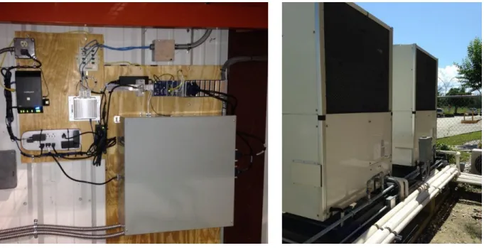
The indoor and outdoor units were already equipped with sensors to measure temperature, pressure, engine rpm, an electronic expansion valve (EEV) position and other operating parameters as shown in Figure C.1. The operational data was recorded on a local computer in a proprietary file format provided by the manufacturer. Additional sensors were installed to measure the temperature/humidity of the zones, refrigerant flow rates, natural gas consumption, and electricity use. A data acquisition system (NI-cDAQ9138) with an onboard computer to run a local data server for recording operation data was also installed (Figures 12, 13). Sensors were installed and connected to the data logger as shown in Figure 14.

G EHP 1 G EHP 2 G EHP 3 G E H P 4 6 TR 8 TR 1 TR 1 TR 4 TR 6 TR 6 TR

(36)

Figure 12. Remote data logging system Figure 13. 8-ton units housing condenser and gas-engine

A second server was setup at the University of South Florida to store the data remotely from the on-site server. The instantaneous performance data was stored locally and then transferred every day to the USF server in batches to provide enough redundancy in times of network failures.

(37)

Table 2 presents the specifications of the additional sensors installed to measure the ambient conditions, refrigerant flow, temperature, humidity, pressure, gas consumption and the indoor comfort along with their rated accuracy. Figure 15 shows the location of the sensors in each GEHP unit that provide the operating parameters recorded by the data logger.

Table 2. Measurements sensors accuracy

S. No. Measurement Sensor Type I/O Range Accuracy

1 Power consumption Watt meter 4-20 mA 0 - 5000 W ±0.5% of full scale

2 Refrigerant flow

(Figure 16)

Coriolis meter 4-20 mA 0 - 6500 kg/h ±0.15% liquid and ±0.5% for gas (-40°C to 130°C) 3 Temperature (Figure 18) Temperature sensor 4-20 mA (-)10°C - 120°C ± 0.1°C at 0°C and ± 0.3 at 100 °C 4 Humidity Humidity sensor 4-20 mA 0 - 100 % ± 2% (10-90% RH) at 25°C 5 Gas consumption (Figure 17) Volumetric flow meter Digital counter 0 - 7.8 m3_/h _{± 2% (-28.8°C to 48.8°C)}

6 Pressure Pressure NA 0 - 4.5 MPa ± 2% of full scale

(38)

Figure 16. Krohne 1000 coriolis meter with MFC 300 converter

Figure 17. IMAC system pulser attached to the natural gas flow meter

Figure 18. Dwyer temperature and humidity sensor

Figure 19. cDAQ-9138 data acquisition system

3.1.2Installation of Data Aquisition System

Installation of the sensors and the data acquisition (DAQ) system (Figure 19) was started in the first week of May 2014. Figures 20 and 21 show the installed gas meter and Wattmeters on the site.

The DAQ system displays and records timestamped operating parameters every second from the connected sensors. The data collected is then transferred to a remote server (located at USF, Tampa)

(39)

twice daily and is deleted from the on-site database to clear the limited onboard memory. This approach provided us the flexibility of storing operating parameters in a structured database, improving the availability, and usability of the collected data.

Figures 22 and 23 show the installed data logger and the Wattmeter inside a safe enclosure. Krohne 1300 refrigerant flowmeters were connected to the data logger and were externally powered (Figure 24). Figure 25 shows the completed instrumentation of the GEHP outdoor units wired and connected to record the energy input and flow rate.

3.1.3 LabView Program

A LabVIEW program was developed to record data remotely with the following features: • Recording the instantaneous and timestamped values from each sensor every second; • Connecting to the remote PostgreSQL server and writing the data;

• Writing scaled and unscaled values of the sensors incorporating unit conversion.

Figure 22. Wattmeters for the AHU's _{Figure 23. Data logging system}

Figure 24. Refrigerant flow meters wired and connected to the DAQ system

Figure 25. DAQ logging installation inside the warehouse

(40)

The development of the program to capture the data took about a month of testing and debugging with the final representative tool as shown in Appendix Figures C.2 and C.3. This program was configured to record all the additional sensors installed for this study. The LabVIEW program was capable of running locally on the data logging system and recording data from the new sensors on a PostgreSQL database. The native GEHP data logger was used for recording all the pre-existing sensors within the GEHP and AHU units.

3.2Data Collection

The data collection at the FPU site started on May 9,2014, which was tested and commissioned on May 30, 2014 (Figure 26). The GEHP data logger captured the operating parameters in 108 fields from the outdoor unit and 20 parameters from the air-handling units that were time-stamped every second. The structure of instantaneous data record is available from the ‘*.AnD’ files generated as shown in Appendix C.2.

(41)

A select number of operational parameters were used to estimate the energy consumption and cooling delivered from the collected data of each GEHP unit. The sequence of operations involved in the periodic data collection and migration is as follows:

• Connection triggered to field data logger by the server, • Flag data ‘to be copied’ on the host computer,

• Move data to USF server, • Flag data as ‘copied,'

• Check data for correctness and completeness after copy process, • Flag data on CERC data logger as copied,

• Delete the data copied in the last transaction from field database, • Disconnect from the remote data logger.

3.3 Data Processing and Synchronization

The native GEHP data logging tool was highly unstable and vulnerable to power failures resulting in loss of data without alerts to the operator. This data was collected in a proprietary ‘*.AnD’ file format that was not readable unless converted to separate CSV files using a manufacturer provided program (each file had 3600 rows of data from the outdoor and indoor units). The indoor unit data file did not have a timestamp and hence merging the data to the outdoor unit file for correct interpretation was deemed necessary. Procedures were developed for conversion as explained in Appendix C.2.

The PostgreSQL database structure of both the datasets is shown in Figure 27, where ‘sensor_data_backup’ is the table for all the data collected through CERC data logging procedures and GEHP1 through 4 are the tables with the data gathered by the native GEHP data logger. The CERC database included all the processed data from all sources with correct timestamps for analysis. Figure 28 details the communication infrastructure deployed to perform this task continuously.

(42)

Figure 27. Schema of USF database

Figure 28. Source and host database communication setup for USF server 3.4 Analysis

Refrigerant–side capacity measurement technique was used to estimate the cooling delivered by each GEHP unit. During Operation, as the refrigerant passes through the evaporator, the specific enthalpy change in the process was calculated using the temperature and pressure measured at the inlet and outlet of the coil.

(43)

The evaporator-side heat delivery rate is found from the relation:

𝑄𝑒𝑣𝑎𝑝 = 𝑚̇(ℎ𝑜− ℎ𝑖)

where ṁ is the refrigerant mass flow rate

ℎ𝑜 = ℎ𝑣𝑎𝑝(𝑇𝑜, 𝑃𝑜) vapor enthalpy at the evaporator exit, and

ℎ𝑖 = ℎ(𝑇𝑖, 𝑃𝑖) enthalpy of two phase mixture at the evaporator inlet

The thermodynamic properties of refrigerant R410a were acquired from REFPROP© for all calculations [59][60]. The electric energy consumed by each GEHP unit is the sum of all the electricity during selected period is found by integrating the power over the period as:

𝐸𝑙𝑒𝑐𝑡𝑟𝑖𝑐 𝑒𝑛𝑒𝑟𝑔𝑦 𝑢𝑠𝑒𝑑 𝑏𝑦 𝑒𝑎𝑐ℎ 𝐺𝐸𝐻𝑃 = ∫ 𝑊𝑒𝑑𝑡

The energy from the natural gas consumed is given by

𝑇𝑜𝑡𝑎𝑙 𝑒𝑛𝑒𝑟𝑔𝑦 𝑓𝑟𝑜𝑚 𝑁𝐺 𝑢𝑠𝑒𝑑 = ∫ 𝑊𝑛𝑔𝑑𝑡

The cooling/heating delivered is calculated as:

𝑞𝑐𝑜𝑜𝑙/ℎ𝑒𝑎𝑡= 𝑚̇(ℎ𝑜− ℎ𝑖)

𝐶𝑂𝑃 = 𝐶𝑜𝑜𝑙𝑖𝑛𝑔

𝐸𝑛𝑒𝑟𝑔𝑦 𝐼𝑛𝑝𝑢𝑡

where We=energy from electricity

Wng=energy from natural gas

The natural gas consumed by each GEHP unit was used as the prediction baseline for annual performance. Figure 29 shows the monthly natural gas consumption for the four GEHP units at DeBary, FL during the study period. It was observed that the natural gas consumption of the GEHP1 was lowest among all the units. However, this does not imply that this unit performed most efficiently. The COP for each GEHP unit was used as the performance indicator in this study during field operation.

Typically, the performance of heat pumps is measured by calculating the coefficient of performance (COP) for cooling or heating application, which is the ratio of the delivered cooling to the primary energy used.

(44)

Figure 29. Monthly natural gas consumption by the four gas heat pumps

In the case of a GEHP system, the energy input is from natural gas as compared to electricity in conventional heat pumps widely used in the sector. Therefore, a direct comparison of such systems is difficult, unless it is based on the primary energy input. Hence, for comparative analysis, COPunit is

considered which excludes the electricity use.

𝐶𝑂𝑃𝑢𝑛𝑖𝑡 =

𝐶𝑜𝑜𝑙𝑖𝑛𝑔 𝑑𝑒𝑙𝑖𝑣𝑒𝑟𝑒𝑑

𝑃𝑟𝑖𝑚𝑎𝑟𝑦 𝑒𝑛𝑒𝑟𝑔𝑦 𝑖𝑛𝑝𝑢𝑡 𝑓𝑟𝑜𝑚 𝑓𝑢𝑒𝑙

The indoor AHU’s and the condenser fans use electricity for both electric heat pumps and gas heat pumps. The technological difference between the two systems is the type of energy used to drive the compressor, which is gas in case of the GEHP units, whereas electricity for the electric heat pumps. Therefore, for a meaningful comparison of the performance. COPunit is calculated as the ratio of the

cooling/heating delivered to the primary energy that is natural gas in the current study.

Figure 30 shows the electricity consumption of the GEHP4 and the corresponding air handling units (AHU) during the month of August 2014. As the compressor is driven by a natural gas based gas-engine, the electricity used by the outdoor units was significantly lower than the corresponding AHU. In a

0 1000 2000 3000 4000 5000 6000 7000 8000

May-14 Jul-14 Aug-14 Oct-14 Dec-14 Jan-15 Mar-15

N at u ra l gas con su m p tio n (k Wh ) GHP1 GHP2 GHP3 GHP4

(45)

complete system, the electricity consumed by a condenser fan is considerably lower than electricity used by AHU.

Figure 30. Electricity use by the GEHP1 indoor and outdoor units for the month of August-2014 In a vapor-compression heat pump systems, the electrical consumption of fans and other auxiliary components of a condensing unit and AHU’s for a heat pump are identical whether the heat pump is a traditional electric or based on the natural gas engine. Hence, the electricity used by the outdoor unit fan is excluded from the calculation of COPunit for meaningful comparison which is usually less than 3% of the

natural gas use.

3.5 Uncertainty in COP Calculation

Table 2 presents the sensors and their measurement accuracy used in this study. The uncertainty in calculated COPunit is determined based on the following equation [61].

𝑊𝐶𝑂𝑃= [( 𝑑𝐶𝑂𝑃 𝑑𝑥1 ∗ 𝑤1) 2 + (𝑑𝐶𝑂𝑃 𝑑𝑥2 ∗ 𝑤2) 2 + (𝑑𝐶𝑂𝑃 𝑑𝑥3 ∗ 𝑤3) 2 + (𝑑𝐶𝑂𝑃 𝑑𝑥4 ∗ 𝑤4) 2 + (𝑑𝐶𝑂𝑃 𝑑𝑥5 ∗ 𝑤5) 2 ] 1/2

where x=measured variable (temperature, refrigerant flow rate, gas consumption, enthalpy, and pressure) 0 5 10 15 20 25 1-A u g 2-A u g 3-A u g 4-A u g 5-A u g 6-A u g 7-A u g 8-A u g 9-A u g 10-A u g 11 -A u g 12-A u g 13-A u g 14-A u g 15-A u g 16-A u g 17-A u g 18-A u g 19-A u g 20-A u g 21-A u g 22 -A u g 23-A u g 24-A u g 25-A u g 26-A u g 27-A u g 28-A u g 29-A u g 30-A u g 31-A u g Ele ctricity u se (kWh ) GEHP1 AHU

(46)

W=uncertainty associated with each measurement

Assuming a confidence interval of the measurement devices to be within 95% and using the above relation, the maximum uncertainty in COPunit was calculated as ±18.02%. The higher uncertainty is

contributed by the reported refrigerant temperatures by the onboard data logging system. The temperature was reported as whole numbers instead of fractions that resulted in higher uncertainty in COP calculations.

3.6Field Operation and Performance Results

The performance of the GEHP units was determined by calculating the cooling produced using the refrigerant side capacity method as explained in section 3.4. The heat content of the natural gas (primary energy source) was taken as 1,016 Btu/ft3_{for calculations [62]. Natural gas SI engine coupled with a}

compressor producing the mechanical work required in a GEHP system. Each unit of primary energy used in the SI engine produce some units of cooling in the building zones, which varied based on the local weather and load conditions. During the summer season, the average COPunit of the GEHP over a weeks’

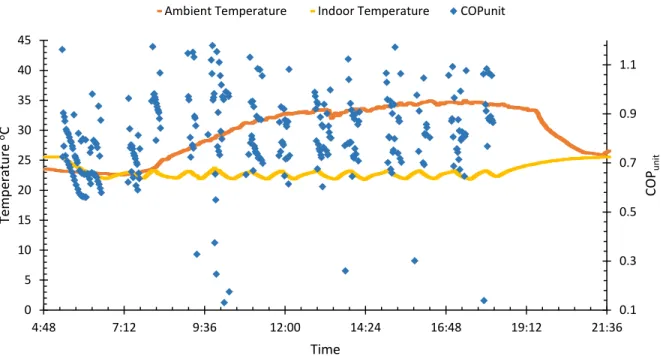
time was found as shown in Figure 31.

The instantaneous COPunitof the GEHP’s varied during this period from 0.1 to 1.4 during the

GEHP’s daily operation. Observed COPunit low values are primarily during the system idle mode once the

setpoint temperature is reached and higher values are found when the full load operation is triggered as shown in Figure 31. It was also observed that during hot and humid days, the GEHP running time significantly increased resulting in higher COPunit.

The operating parameters of one GEHP unit for a typical day are presented in Figure 32, while the performance indicator (COPunit) is shown in Figure 33. The GEHP operation was found to be unsteady, and

hence, resulted in fluctuations in the recorded data points. The natural gas consumption and cooling produced was intermittent as the GEHP units cycle ‘on’ and ‘off’ frequently while controlling the indoor temperature.

(47)

Figure 31. Field performance during summer

Figure 32. Cooling delivered and energy use for a typical summer day

The operation schedule at the study location was set between 5 a.m. - 7 p.m. for all GEHP units. During morning hours, the GEHP units ran continuously and for longer durations due to the accumulated thermal load overnight. However, during later hours of operation, the GEHP units provide cooling for shorter cycles. The total cooling delivered during such operations ranged between 165 to 365 Wh.

15 65 115 165 215 265 315 365 0 5 10 15 20 25 30 35 40 45 4:48 7:12 9:36 12:00 14:24 16:48 19:12 21:36 Wh Te m p era tu re oC Time

(48)

Figure 33. The performance of the GEHP on a typical summer day

The GEHP units operated continuously during the initial hours of a typical day, with the highest gas engine RPM of 1950. The calculated COPunit during such operation was found to be steady, and its

variation with ambient temperature is shown in Figure 34. As expected, it was observed that as the ambient temperature increases the corresponding COPunit declines.

Figure 34. Effect of ambient temperature on the COP achieved at 1950 RPM

0.1 0.3 0.5 0.7 0.9 1.1 0 5 10 15 20 25 30 35 40 45 4:48 7:12 9:36 12:00 14:24 16:48 19:12 21:36 COP u n it Te m p era tu re oC Time

Ambient Temperature Indoor Temperature COPunit

0.0 0.1 0.2 0.3 0.4 0.5 0.6 0.7 0.8 0.9 1.0 20 22 24 26 28 30 32 34 36 38 COP Un it Ambient Temperature o_C

(49)

Figure 34 presents the variation of COPunit with the temperature at maximum rpm found during

the study. However, the performance of all the GEHP units does not reflect a similar trend. This variation was due to the difference in configuration of each GEHP unit and corresponding thermal zones during operation (Figure 11).

3.7 Measured Performance

Monthly performance of the four GEHP units during the summer months is summarized in Table 3 to 6 below. The data collected for GEHP2 during June-14 of was not complete and, therefore, the COP could not be determined. The system COP presented in Table 3 is the ratio of cooling produced divided by the combined electrical and natural gas energy used by the outdoor unit. The complete measured data summary is provided in Appendix Table C.3.

Table 3. June performance of GEHP units Jun-14 Natural Gas

use (kWh) Electricity Use (kWh) Total Energy Input (kWh) Cooling (kWh) Average COPunit Average System COP GEHP1 3661 101 3763 2478 0.68 0.66

GEHP2 4245 #N/A 4245 #N/A #N/A #N/A

GEHP3 5414 145 5560 4586 0.85 0.82

GEHP4 3780 92 3872 1705 0.45 0.44

#N/A-Data not available

Table 4. July performance of GEHP units Jul-14 Natural Gas

use (kWh) Electricity Use (kWh) Total Energy Input (kWh) Cooling (kWh) Average COPunit Average System COP GEHP1 3928 104 3969 2541 0.65 0.63 GEHP2 4372 117 4418 1687 0.39 0.38 GEHP3 5726 149 5782 4525 0.79 0.77 GEHP4 6179 130 6210 2567 0.42 0.41

Table 5. August performance of GEHP units Aug-14 Natural Gas

(50)

Table 6. September performance of GEHP units Sep-14 Natural Gas

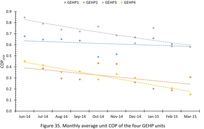
Figure 35. Monthly average unit COP of the four GEHP units

During the summer operation, GEHP3 had achieved the highest COPunit among the four units, and

GEHP2 was at the lowest COPunit, as shown in Figure 35. The monthly performance data is summarized for

all four units in Appendix C (Table C.3). The observed variations were due to many system variables that are different for each unit and hence they influence the performance differently.

3.8 Comparison with Laboratory and Other Field Experiments

Zaltash et al. [63] 2007 reported COP of GEHP units tested in a laboratory under a controlled environment. Sohn et al. [58] in 2008 reported field operation and performance of six GEHP units. Performance reported in these studies was used for comparison for the current study. Figure 36 shows

0.0 0.1 0.2 0.3 0.4 0.5 0.6 0.7 0.8 0.9

Jun-14 Jul-14 Aug-14 Sep-14 Oct-14 Nov-14 Dec-14 Jan-15 Feb-15 Mar-15

COP

Un

it

(51)

the comparative performance (cooling COP) of GEHP unit obtained in laboratory experiments by Zaltash et al., the field testing results by Sohn et al. and the COPunit found in the current research.

Figure 36. Measured performance compared with other studies

The decline in the COPunit in the present study with an increase in ambient temperature agrees

with the reported research. However, the COPs reported by Zaltash et al. and Sohn et al. are almost double the COPunit obtained from the GEHP units studied in the current work. It should be noted that the

conditions in all these three studies are different and hence an exact comparison is not possible. 3.9Energy Efficiency of GEHP Operations

To understand the observed low performance during field operation, the individual performance of various components of the system was determined using the maximum load operation data for analysis. The fuel input, compressor output and cooling delivered were calculated which were then used to estimate the delivered performance. The overall efficiency of the engine and compressor unit is a

0.1 0.3 0.5 0.7 0.9 1.1 1.3 1.5 1.7 15 20 25 30 35 40 45 50 COP u n it Ambient Temperature o_C