Volume 17 | Issue 1 Article 19
7-11-2018
A Bayesian Beta-Mixture Model for Nonparametric
IRT (BBM-IRT)
Ethan A. Arenson
University of Illinois at Chicago, [email protected]
George Karabatsos
University of Illinois at Chicago, [email protected]
Follow this and additional works at:https://digitalcommons.wayne.edu/jmasm
Part of theApplied Statistics Commons,Social and Behavioral Sciences Commons, and the Statistical Theory Commons
Recommended Citation
Arenson, Ethan A. and Karabatsos, George (2018) "A Bayesian Beta-Mixture Model for Nonparametric IRT (BBM-IRT),"Journal of Modern Applied Statistical Methods: Vol. 17 : Iss. 1 , Article 19.
DOI: 10.22237/jmasm/1531318047
Cover Page Footnote
This research is part of Arenson's Ph.D. dissertation. Karabatsos is his Ph.D. advisor, and corresponding author. Karabatsos thanks Stephen G. Walker for helpful discussions about beta mixture modeling, and thanks two anonymous reviewers for their suggestions to improve the presentation of this article. This research was supported by NSF grants SES-1156372 and SES-0242030 (PI: Karabatsos).
Erratum
In the original published version of this article, equations (A1) through (A6) were incorrectly labelled (A9) through (A14). This has been corrected.
doi: 10.22237/jmasm/1531318047 | Accepted: September 5, 2017; Published: July 11, 2018. Correspondence: George Karabatsos, [email protected]
A Bayesian Beta-Mixture Model for
Nonparametric IRT (BBM-IRT)
Ethan A. Arenson
University of Illinois at Chicago Chicago, IL
George Karabatsos
University of Illinois at Chicago Chicago, IL
Item response models typically assume that the item characteristic (step) curves follow a logistic or normal cumulative distribution function, which are strictly monotone functions of person test ability. Such assumptions can be overly-restrictive for real item response data. A simple and more flexible Bayesian nonparametric IRT model for dichotomous items is introduced, which constructs monotone item characteristic (step) curves by a finite mixture of beta distributions, which can support the entire space of monotone curves to any desired degree of accuracy. An adaptive random-walk Metropolis-Hastings algorithm is proposed to estimate the posterior distribution of the model parameters. The Bayesian IRT model is illustrated through the analysis of item response data from a 2015 TIMSS test of math performance.
Keywords: Bayesian modeling, item response theory, MCMC, adaptive Metropolis, TIMSS data
Introduction
Item Response Theory (IRT) is a successful enterprise that provides a class of useful statistical models for the analysis of item response data (Hambleton & Swaminathan, 1985; van der Linden, 2016).
Any IRT model posits a probabilistic relationship between each person's response to each test item based on person ability and item parameters. To explain, let Yni be the item response random variable for person n and test item i with persons
and items indexed by n = 1,…, N and by i = 1,…, I (respectively). Nearly all IRT models make at least the following three assumptions (Junker & Sijtsma, 2001):
1) Unidimensionality: Person ability, θ, is real-valued (possibly multidimensional);
2) Local Independence: The conditional distribution of the responses to the test items satisfies:
(
1 1)
(
)
1 Pr , , | Pr | I I I i i i Y y Y y Y y = = = =
= (1)3) Monotonicity: The Item Step Response Function (ISRF),
(
)
Pr Yi k| monotone non-decreasing in for i=1, , , I k=0,1,,Ki (2) with Pr(Yi = 1 | θ) = Pr(Yi > k | θ) the Item Characteristic Curve (ICC) for a
dichotomous (Ki = 1) items.
Then, θ has positive correlation with the total test score
1 I
i i= Y
(van der Ark & Bergsma, 2010).These three assumptions exactly describe the nonparametric, monotone homogeneity (MH) IRT model (Mokken, 1971). It is the most general monotone IRT model which nests the 4-parameter logistic model (Hambleton & Swaminathan, 1985); the graded response logistic model (Samejima, 1969) and all other monotone IRT models (Van der Ark, 2001) are special cases.
The focus of the current study is on unidimensional IRT for dichotomous items. Although parametric IRT models provide a certain elegance and computational simplicity, nonparametric IRT models are more informative and more closely describe the true item response functions that underlie real data. This contrasts with parametric IRT models which assume that ICCs follow a parametric distribution function, such as the logistic function (e.g., van der Linden, 2016). Also, a nonparametric IRT model can provide better fit to data compared to parametric IRT models, be used to evaluate the fit of the latter, and promote coherent statistical inference from a Bayesian perspective (Karabatsos & Walker, 2009a).
Various MH models were proposed, defined by generalized linear models that specify the ICC as an inverse-link function parameter that is monotone in θ, and give support to the entire space of monotone cumulative distribution functions (c.d.f.s). Qin (1998) and Duncan and MacEachern (2008) proposed a Bayesian nonparametric (BNP) model that constructed monotone ICCs by a Dirichlet process centered on a 2-parameter logistic IRT model. Karabatsos (2016) modeled ICCs by a BNP infinite-mixture of normal c.d.f.s for the latent item response variables, with person- and item-dependent mixture weights. Karabatsos and Sheu (2004) and
Tijmstra, Hessen, van der Heijden, and Sijtsma (2013) proposed isotonic regression, using a Bayesian and frequentist approach (respectively), assuming discrete-valued
θ. Luzardo and Rodriguez (2015) used classic nonparametric kernel regression methods to estimate monotone ICCs. Finally, Karabatsos and Walker (2009b, 2010) presented a BNP beta-mixture model for test score equating.
In this study, a simple and flexible BNP IRT model is proposed for dichotomous items and continuous-valued ability (θ), extending a generalized linear model with unknown link function parameter (Mallick & Gelfand, 1994). Our BNP IRT model maps the unidimensional ability parameter θ from the real-line onto (0, 1), and constructs a (random) monotone ICC (inverse-link) by a flexible finite-mixture of beta c.d.f.s. In fact, any smooth c.d.f. on (0, 1) can be approximated arbitrarily-well by a suitable finite mixture of beta c.d.f.s (Diaconis & Ylvasiker, 1985).
The Bayesian beta-mixture IRT model (BBM-IRT) is more flexible than traditional parametric IRT models, which make logistic or normal distributional assumptions about the ICCs. The BBM-IRT model allows one to estimate more accurately estimate ICCs which may have shapes that would be considered misfitting under the traditional models. Also, the BBM-IRT model is more parsimonious and computationally feasible than previous BNP IRT models which can employ thousands of parameters.
The BBM-IRT model is completed by the specification of a joint prior distribution for the person ability parameters and the item-level mixture weight parameters, and the number of mixture components. Our IRT model is a flexible, approximate BNP model, because it makes use of finite instead of infinite mixtures to attain more computational tractability. A mixture of 3 to 4 beta distributions was believed to provide adequate modeling flexibility (Mallick & Gelfand, 1994). This article shows that a mixture of 10 beta distributions, per test item, can provide gains in data fit for IRT modeling.
The next section presents our BBM-IRT model, and statistics for assessing the model’s goodness-of-predictive fit. A simple iterative Markov chain Monte Carlo (MCMC) algorithm (Appendix) can be used for estimating the posterior distribution of the model parameters and their functionals of interest. The following section illustrates our IRT model through the analysis of a 20-item math exam data set, from a 2015 Trends in International Mathematics and Science Study (TIMSS) assessment of 8th grade students. The final section discusses conclusions and
Methodology: BBM-IRT Model
Let Yni∈ {0, 1} be a dichotomous item-response variable for person n and test item
i. For a matrix of realized item response data, Y = (yni)N×I, our BBM-IRT model is
defined by
(
)
(
(
)
)
(
)
(
)
(
)
(
)
( )
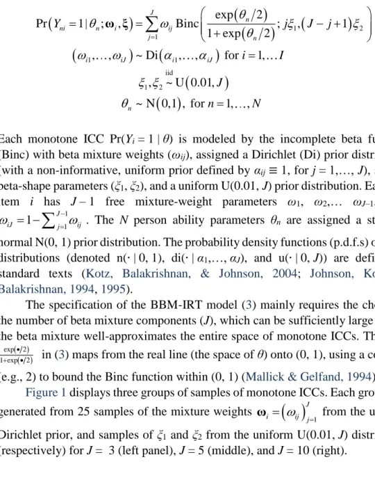
1 2 1 1 1 iid 1 2 exp 2 Pr 1| ; , Binc ; , 1 1 exp 2 , , ~ Di , , for 1, , ~ U 0.01, ~ N 0,1 , for 1, , J n ni n i ij j n i iJ i iJ n Y j J j i I J n N = = = − + + = =
ω ξ (3)Each monotone ICC Pr(Yi = 1 | θ) is modeled by the incomplete beta function
(Binc) with beta mixture weights (ωij), assigned a Dirichlet (Di) prior distribution
(with a non-informative, uniform prior defined by αij≡ 1, for j = 1,…, J), scaling
beta-shape parameters (ξ1, ξ2), and a uniform U(0.01, J) prior distribution. Each test
item i has J – 1 free mixture-weight parameters ω1, ω2,… ωJ–1, with
1 1 1 J iJ j ij − =
= −
. The N person ability parameters θn are assigned a standardnormal N(0, 1) prior distribution. The probability density functions (p.d.f.s) of these distributions (denoted n(∙ | 0, 1), di(∙ | α1,…, αJ), and u(∙ | 0, J)) are defined in
standard texts (Kotz, Balakrishnan, & Johnson, 2004; Johnson, Kotz, & Balakrishnan, 1994, 1995).
The specification of the BBM-IRT model (3) mainly requires the choice of the number of beta mixture components (J), which can be sufficiently large so that the beta mixture well-approximates the entire space of monotone ICCs. The term
( ) ( ) exp 2 1 exp 2
•
+ • in (3) maps from the real line (the space of θ) onto (0, 1), using a constant (e.g., 2) to bound the Binc function within (0, 1) (Mallick & Gelfand, 1994).
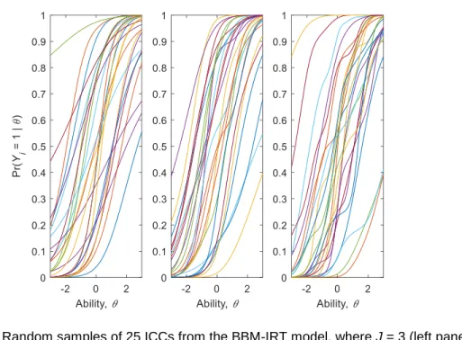
Figure 1 displays three groups of samples of monotone ICCs. Each group was generated from 25 samples of the mixture weights
( )
1 J i = ij j=
ω from the uniform Dirichlet prior, and samples of ξ1 and ξ2 from the uniform U(0.01, J) distribution
Figure 1. Random samples of 25 ICCs from the BBM-IRT model, where J = 3 (left panel),
J = 5 (middle), and J = 10 (right)
The ICCs in the left panel (J = 3) resemble the ICCs of a 2-parameter logistic (2PL) IRT model. If J = 1 and ξ = ξ1 = ξ2, then the BBM-IRT model reduces to a
Rasch-type IRT model with common item discrimination parameter, ξ. The middle and right panels show that, as J is increased, the ICCs become wigglier and more flexible. The right panel shows that J = 10 mixture components defines a BBM-IRT model that broadly and flexibly supports the entire space of monotone ICCs. The BBM-IRT model is thus a monotone IRT model, and a highly-parametric BNP model (Müller & Quintana, 2004).
For the BBM-IRT model (3), the joint posterior p.d.f. (distribution) of the model parameters,
(
( ) ( )
1 2)
1, 1, , N I n n i i = = =ζ ω , is given by (up to a normalizing constant)
(
)
(
)
(
)
(
)
(
) (
) (
)
1 1 1 1 1 2 1 1 π | Pr 1| ; , 1 Pr 1| ; , n | 0,1 di | , , u | 0, u | 0, ni ni N I y y ni n i ni n i n i N I n i i iJ n i Y Y J J − = = = = = − =
ζ Y ω ξ ω ξ ω (4)with ICCs Pr(Yni = 1 | θn; ωi, ξ) defined by (3) and corresponding posterior c.d.f.
Π(ζ | Y). The model’s posterior predictive expectation (E) and variance (V) of the item response variable Yni is given by (for all persons n = 1,…, N and all items
i = 1,…, I)
( )
(
) (
)
( )
(
)
(
)
(
)
E Pr 1| ; , Π | , V Pr 1| ; , 1 Pr 1| ; , Π | NI ni ni n i NI ni ni n i ni n i Y Y d Y Y Y d = = = = − =
ω ξ ζ Y ω ξ ω ξ ζ Y (5)Using the D(m) criterion, it is possible to compare the predictive fit between BBM-IRT models to the data, which may differ by choice of J or prior distribution. Specifically, for each model indexed by m = 1,…, M, the D(m) criterion measures posterior predictive model fitness to the data Y (Laud & Ibrahim, 1995), and is defined by
( )
(
)
2(
)
1 1 D E | V | N I ni NI ni NI ni n i m y Y m Y m = = =
− + (6)The first term in (6) measures goodness-of-fit to the sample data (Y). The second term is a model complexity penalty. Among the M Bayesian models compared, the model with the best predictive utility for the given data set (Y) is identified as the model with the smallest value of D(m). The D(m) criterion is often used in Bayesian data analysis practice, and is easier to compute compared to other criteria.
The fit of a single BBM-IRT model (m) can be assessed by standardized item-response residuals:
(
)
(
)
1 2 E | , for 1, , , 1, , | ni NI ni ni NI ni y Y m z n N i I V Y m − = = = (7)An absolute residual |zni| exceeding 2 or 3 suggests that the response is an outlier
under the model.
The BBM-IRT model’s posterior distribution (4) and the posterior predictive quantities (5)-(7) can be estimated by using an adaptive random-walk Metropolis-Hastings MCMC algorithm. See the Appendix for details.
Results: TIMSS Data Analysis
The BBM-IRT model is illustrated through the analysis of 2015 TIMSS data on a basic math and algebra assessment of 716 American 8th grade students. The data set contains the students' individual responses to 20 math items, each response scored as correct (Yni = 1) or incorrect (Yni = 0). The data contains 639 unique item
response patterns on the 20-item test. The Supplementary material of this article provides the TIMSS data set and the descriptions of the 20 items. It also provides the MATLAB code files that were used to run the MCMC sampling algorithm to analyze the TIMSS data using BBM-IRT and the 2PL IRT models, and to produce the results reported here.
The BBM-IRT model was fit to the TIMSS data using J = 10 components, a uniform Dirichlet prior for the mixture weights of the test items, and a standard normal N(0, 1) prior for the 716 student math ability parameters (respectively). The posterior distribution of the model was estimated by a 100K iteration run of the MCMC sampling algorithm (Appendix).
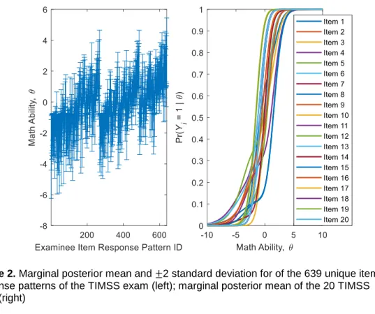
Figure 2. Marginal posterior mean and ±2 standard deviation for of the 639 unique item response patterns of the TIMSS exam (left); marginal posterior mean of the 20 TIMSS ICCs (right)
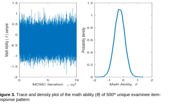
Figure 3. Trace and density plot of the math ability (θ) of 500th unique examinee
item-response pattern
The left panel of Figure 2 presents the marginal posterior means and ±2 standard deviations of the person ability parameter for each of the 639 unique item response patterns. The right panel presents the marginal posterior mean estimates for the 20 ICCs of the test items. It shows multiple crossings among the 20 ICCs, with some ICCs fluctuating more than others. These ICC results exhibit the flexibility and monotonicity of the BBM-IRT model, which may be misdiagnosed as outlying according to traditional IRT models that assume more restrictive logistic or normal ICCs.
Some of the estimated ICCs in Figure 2 have non-zero lower asymptotes, indicating the presence of guessing among low-ability examinees for these items. Thus, the BBM-IRT model (and its MCMC algorithm) can account for lucky-correct item responses among low-ability examinees. It does so while avoiding the issues of estimating the chance parameter in the three-parameter logistic IRT model, using either marginal maximum likelihood or Bayesian methods.
The following two diagnostic methods (Flegal & Jones, 2011) can be used to assess the convergence of the 100K MCMC parameter samples to the IRT model's exact posterior distribution. First, trace plots were used to evaluate the mixing (sampling independence) of the MCMC chain of each model parameter, over the 100K iterations. Second, a non-overlapping batch means analysis of the chain was performed to calculate the Monte Carlo 95% confidence interval half-width
(95%MCCIhw) for each marginal posterior mean and posterior variance estimate. MCMC convergence can always be improved by running the MCMC chain beyond 100K sampling iterations.
Figure 3 illustrates these two MCMC convergence diagnostic methods for
θ(500), the ability parameter corresponding to the 500th unique item response pattern
in the TIMSS data. The left panel of Figure 3 presents the trace plot of θ(500) over
the 100K MCMC sampling iterations. This plot supports good mixing and (near) sampling independence of the chain. The right panel presents a kernel density estimate of the marginal posterior distribution of θ(500). The marginal posterior
mean and variance of θ(500) is –0.3 and 0.1, with corresponding 95%MCCIhw
values of 0.00 and 0.00. It can be concluded that the MCMC samples of the parameter θ(500) have adequately converged to its marginal posterior distribution.
Similar conclusions about MCMC convergence can be reached about the ability parameter for each of the 639 unique item response patterns, and about points on the ICC curve, for each individual test item.
For comparison, several different versions of the BNP-IRT model were fit to the TIMSS data. They employed either J = 3, 5, and 10 mixture components; either a standard normal N(0, 1) prior distribution, a left-skewed normal mixture prior 0.25 × N(–1, 1) + 0.75 × N(1, 1), or a right-skewed normal mixture prior 0.75 × N(–1, 1) + 0.25 × N(1, 1) on the ability parameters; and a uniform Dirichlet prior. The Bayesian 2PL model was also fit to the data, defined by
(
)
(
1)
Pr 1| , , for 1, , and 1, , 1 exp ni n i i i n i Y n N i I = = = = + − + (8)with an N(0, 1) prior for the person ability parameters (θn), an N(0, 4) prior for the
item difficulty parameters (βi), and an N(0, 1/4) prior for the log slope log(αi)
parameters (respectively) suggested for analyzing data from large scale testing (Patz & Junker, 1999). The 2PL model was fit using an adaptive version of a published random-walk Metropolis MCMC algorithm (Patz & Junker, 1999). To estimate the posterior distribution of each of these compared IRT models, the MCMC algorithm was run for 100K iterations. In each case, MCMC convergence analyses can be shown to yield similar results as before.
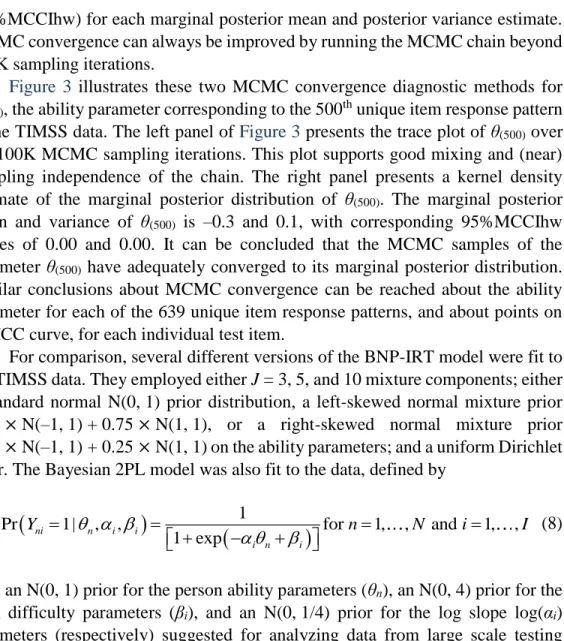
For each IRT model, Table 1 summarizes the posterior predictive model fit statistic, D(m), and the proportion of posterior predictive standardized residuals (zni)
greater than 2 (and 3) in absolute magnitude. By considering both criteria, we find that the BBM-IRT model with J = 10 mixture components obtained the best
had about twice the number of outliers with residuals |zni| > 3. In terms of D(m), the
BBM-IRT model fit best under symmetric priors for the ability parameters.
Table 1. A comparison of the predictive fit between different IRT models
Proportion residuals Bayesian IRT Model D(m) |zni| ≥ 2 |zni| ≥ 3
BBM-IRT, J = 3 4752 0.03 0.005
BBM-IRT, J = 5 4643 0.03 0.006
BBM-IRT, J = 10 4625 0.03 0.004
BBM-IRT, J = 3, left-skewed θ prior 4729 0.03 0.004 BBM-IRT, J = 5, left-skewed θ prior 4666 0.03 0.005 BBM-IRT, J = 10, left-skewed θ prior 4637 0.02 0.004 BBM-IRT, J = 3, right-skewed θ prior 4702 0.03 0.004 BBM-IRT, J = 5, right-skewed θ prior 4653 0.03 0.005 BBM-IRT, J = 10, right-skewed θ prior 4640 0.02 0.004
2PL Model 4717 0.03 0.010
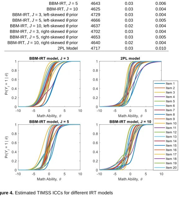
Figure 4 compares the marginal posterior mean estimates for the 20 ICCs between the BBM-IRT models with J = 3, 5, and 10 components and the Bayesian 2PL model (respectively), and an N(0, 1) prior for the ability parameters. Compared to the ICCs of the 2PL model, the ICCs of the 3-component BBM-IRT model were most similar, and the ICCs of the 10-component BBM-IRT model were most dissimilar.
Conclusions
A novel monotone BBM-IRT model was introduced for dichotomous item responses and unidimensional ability. It provides a useful compromise between more restrictive parametric IRT models and more flexible and computationally intensive BNP models. The BBM-IRT flexibly models each ICC by a finite mixture of beta c.d.f.s, which approximately support the entire space of monotone ICCs. Posterior inference of this model is possible through the application of a simple adaptive Metropolis MCMC algorithm. The usefulness of the BBM-IRT model was illustrated through the analysis of item response data from a TIMSS math assessment.
The BBM-IRT model shows promise for future research opportunities. For instance, one can extend this model to handle the analysis of polytomous item response data, by coding each observed polytomous response to a set of binary codes (Begg & Gray, 1984), or by replacing the Bernoulli kernel (incomplete Beta function) with a binomial or multinomial kernel in (3). In addition one can extend this model to handle multidimensional ability by assigning each person separate ability parameters for different subgroups of test items that measures different traits.
References
Atchadé, Y., & Rosenthal, J. (2005). On adaptive Markov chain Monte Carlo algorithms. Bernoulli, 11(5), 815-828. doi: 10.3150/bj/1130077595
Begg, C., & Gray, R. (1984). Calculation of polychotomous logistic
regression parameters using individualized regressions. Biometrika, 71(1), 11-18. doi: 10.1093/biomet/71.1.11
Diaconis, P., & Ylvisaker, D. (1985). Conjugate priors for exponential families. The Annals of Statistics, 7(2), 269-281. doi: 10.1214/aos/1176344611
Duncan, K., & MacEachern, S. (2008). Nonparametric Bayesian modelling for item response. Statistical Modelling, 8(1), 41-66. doi:
10.1177/1471082x0700800104
Flegal, J., & Jones, G. (2011). Implementing Markov chain Monte Carlo: Estimating with confidence. In S. Brooks, A. Gelman, G. Jones, & X. Meng (Eds.), Handbook of Markov chain Monte Carlo (p. 175-197). Boca Raton, FL: Chapman and Hall/CRC.
Hambleton, R., & Swaminathan, H. (1985). Item response theory: Principles and applications. New York: Kluwer-Nijhoff.
Johnson, N., Kotz, S., & Balakrishnan, N. (1994). Continuous univariate distributions (2nd ed.) (Vol. 1). New York: Wiley.
Johnson, N., Kotz, S., & Balakrishnan, N. (1995). Continuous univariate distributions (2nd ed.) (Vol. 2). New York: Wiley.
Junker, B., & Sijtsma, K. (2000). Latent and manifest monotonicity in item response models. Applied Psychological Measurement, 24(1), 65-81. doi:
10.1177/01466216000241004
Karabatsos, G. (2016). Bayesian nonparametric IRT. In W. J. van der Linden (Ed.), Handbook of item response theory (Vol. 1) (pp. 323-336). Boca Raton, FL: Chapman & Hall/CRC.
Karabatsos, G., & Sheu, C.-F. (2004). Order-constrained Bayes inference for dichotomous models of unidimensional nonparametric IRT. Applied
Psychological Measurement, 28(2), 110-125. doi: 10.1177/0146621603260678 Karabatsos, G., & Walker, S. G. (2009a). Coherent psychometric modeling with Bayesian nonparametrics. British Journal of Mathematical and Statistical Psychology, 62(1), 1-20. doi: 10.1348/000711007x246237
Karabatsos, G., & Walker, S. G. (2009b). A Bayesian nonparametric approach to test equating. Psychometrika, 74(2), 211-232. doi: 10.1007/s11336-008-9096-6
Karabatsos, G., & Walker, S. G. (2010). A Bayesian nonparametric model for test equating. In A. von Davier (Ed.), Statistical models for equating, scaling, and linking (pp. 175-184). New York: Springer. doi: 10.1007/978-0-387-98138-3_11
Kotz, S., Balakrishnan, N., & Johnson, N. (2004). Continuous multivariate distributions (Vol. 1). New York: John Wiley and Sons. doi: 10.1002/0471722065
Laud, P., & Ibrahim, J. (1995). Predictive model selection. Journal of the Royal Statistical Society. Series B (Methodological), 57(1), 247-262. Available from https://www.jstor.org/stable/2346098
Luzardo, M., & Rodriguez, P. (2015). A nonparametric estimator of a monotone item characteristic curve. In L. A. van der Ark, D. Bolt, W.-C. Wang, A. Douglas, & S.-M. Chow (Eds.), Quantitative psychology research (pp. 99-108). Cham, Switzerland: Springer International Publishing. doi: 10.1007/978-3-319-19977-1_8
Mallick, B., & Gelfand, A. (1994). Generalized linear models with unknown link functions. Biometrika, 81(2), 237-245. doi: 10.1093/biomet/81.2.237
Mokken, R. (1971). A theory and procedure of scale analysis. The Hague, Netherlands: Mouton. doi: 10.1515/9783110813203
Müller, P., & Quintana, F. A. (2004). Nonparametric Bayesian data analysis.
Statistical Science, 19(1), 95-110. doi: 10.1214/088342304000000017
Patz, R., & Junker, B. (1999). A straightforward approach to Markov Chain Monte Carlo methods for item response theory models. Journal of Educational and Behavioral Statistics, 24(2), 146-178. doi: 10.2307/1165199
Qin, L. (1998). Nonparametric Bayesian models for item response data
(Unpublished doctoral dissertation). The Ohio State University, Columbus, OH. Roberts, G., & Rosenthal, J. (2001). Optimal scaling for various Metropolis-Hastings algorithms. Statistical Science, 16(4), 351-367. doi:
10.1214/ss/1015346320
Samejima, F. (1969). Estimation of latent ability using a response pattern of graded scores. Psychometrika, 34(Suppl 1), 1-97. doi: 10.1007/bf03372160
Tijmstra, J., Hessen, D., van der Heijden, P., & Sijtsma, K. (2013). Testing manifest monotonicity using order-constrained statistical inference.
Psychometrika, 78(1), 83-97. doi: 10.1007/s11336-012-9297-x
Van der Ark, L. A. (2001). Relationships and properties of polytomous item response theory models. Applied Psychological Measurement, 25(3), 273-282. doi: 10.1177/01466210122032073
van der Ark, L. A., & Bergsma, W. (2010). A note on stochastic ordering of the latent trait using the sum of polytomous item scores. Psychometrika, 75(2), 272-279. doi: 10.1007/s11336-010-9147-7
van der Linden, W. J. (2016). Handbook of item response theory (Vols. 1-3). Boca Raton, FL: Chapman & Hall/CRC.
Appendix: MCMC Algorithm for BBM-IRT Model
For the BBM-IRT model (3), a 3-step MCMC iterative sampling algorithm is used to estimate the posterior distribution (4) (density) of the N ability parameters and the I ICC parameters. A large number of sampling iterations (S) is run until the algorithm yields a sample that converges (approximately) to a sample from the posterior distribution (MCMC convergence).
The algorithm is initiated at stage s = 0, with model parameter values
(
( )0)
1 0 N n n = ,
(
)
1 1 J ij J j = , for i = 1,…, I ξ1≡ξ2≡ 1, and their proposal variances(
( ))
0 1 0.01 N c n = ,
(
( )0)
1 0.01 I i i = , and(
( )0)
1 0.01 I i = . Also, to speed up computations, the original item response data set Y = (yni)N×I is collapsed into a smaller data set, YC = (yci)C×I, consistingof C≤N unique values of the item response vectors
(
(
1)
)
1
, , C
c = yc ycI c=
y , with frequency counts n1,…, nc,…, nC
(respectively).
Each iteration s∈ {1,…, S} of the MCMC sampling algorithm runs the following three adaptive Metropolis sampling steps, applying the established methodology of Atchadé and Rosenthal (2005):
In Step 1, for each c = 1,…, C independently (concurrently), a candidate ability parameter c s is drawn from the normal N
(
c s−1,sc−1)
proposal distribution. The update c s c s is accepted with probability P cs =min 1,
sc , and otherwise c s c s−1 is set with probability 1−P cs , where
(
)
(
)
( )
(
)
(
)
( )
1 2 1 1 1 1 1 1 2 1 1 1 1 1 1 1 1 1 Pr 1| ; , 1 Pr 1| ; , exp 2 1 Pr 1| ; , 1 Pr 1| ; , exp 2 ui ui ui ui I s s s y s s s y s ci c i ci c i c s i c I y y s s s s s s s ci c i ci c i c i Y Y Y Y − − − − − = − − − − − − − − = = − = − = = − = −
ω ξ ω ξ ω ξ ω ξ (A1)In (A1), a few terms cancel out, including the counts
( )
nc Cc=1, the constants of the normal proposal p.d.f.s, and, the normal proposal p.d.f.s due to their symmetry. Then the proposal variances are updated by 3 1
( )
(
)
min 10 , 1 0.44 s s s c c s c = − − + − toward achieving the optimal acceptance rate of 0.44 (see Roberts & Rosenthal, 2001) over the S MCMC iterations, for c = 1,…, C.
In Step 2, for i = 1,…, I independently (concurrently), a candidate (log) mixture weight parameter
(
)
1logωis =log is, ,iJs is drawn from the J-variate normal proposal distribution, N log
(
(
i −1 s 1, ,iJ − s 1)
, si−1IJ)
. The update ωi s exp log(
ωi s)
is accepted with probability P si =min 1,
si , and otherwise ω is ω is−1 is set with probability 1−P si , where (
)
(
)
( )
(
)
(
)
( )
1 1 1 1 1 1 1 1 1 1 1 1 1 1 1 Pr 1| ; , 1 Pr 1| ; , Pr 1| ; , 1 Pr 1| ; , ui ui ij ui ui ij C y y J s s s s s s s c ci c i ci c i ij s c j i C y y J s s s s s s s c ci c i ci c i ij c j n Y Y n Y Y − − − − = = − − − − − − − = = = − = = = − =
ω ξ ω ξ ω ξ ω ξ (A2)In (A2), the Dirichlet proposal p.d.f. constants and the normal proposal p.d.f. cancel out. Then, the proposal variances are updated by si =min 10 , −3 si−1 +
( )
1s(
si −0.234)
toward achieving the optimal acceptance rate of 0.234 for multidimensional parameters (Roberts & Rosenthal, 2001), for i = 1,…, I.In Step 3, a candidate log
(
1, 2)
s is drawn from the bivariate normal proposal distribution,
(
)
(
1 1 1)
1 2
N log s− , s− ,s− IJ . The update (ξ1, ξ2)[s]≡ exp(log((ξ1, ξ2)*[s]) is accepted with probability P s =min 1,
s ,and otherwise
(
1, 2)
s (
1, 2)
s−1 with probability 1−P s , where
(
)
(
)
(
)
(
)
(
)
(
)
1 1 2 1 1 1 1 1 1 1 1 2 1 1 Pr 1| ; , 1 Pr 1| ; , 0.01 , Pr 1| ; , 1 Pr 1| ; , 0.01 , ui ui ui ui C I y y s s s s s s s s c ci c i ci c i s c i C I y y s s s s s s s s c ci c i ci c i c i n Y Y J n Y Y J − = = − − − − − = = = − = = = − =
ω ξ ω ξ l ω ξ ω ξ l (A3)The uniform prior p.d.f. constants and the normal proposal p.d.f. cancel out of the ratio (A3). Then, the proposal variance is updated by s =min 10 , −3 s−1 +
( )
1 s(
s −0.44)
toward achieving the optimal acceptance rate of roughly 0.44 for two-dimensional parameters (Roberts & Rosenthal, 2001).As a simple by-product of the three-step MCMC algorithm, it is possible to estimate the marginal posterior average and variance of each ability parameter, θc (for c = 1,…, C), and the marginal posterior mean and variance of each ICC,
Pr(Yi = 1 | θ; ωi, ξ), over a chosen fine grid of θ values. Specifically, at each MCMC iteration s∈ {1,…, S}, the marginal
posterior expectation (E) and variance (V) of each θc is updated through Rao-Blackwellization, via the calculations
( )
(
)
( )
( )
( )
(
)
( )
( )
( )
( )
1 2 1 2 2 2 2 ˆ ˆ E 1 E ˆ ˆ E 1 E ˆ ˆ ˆ V E E s s s NI c c NI c s s s NI c c NI c s s s NI c NI c NI c s s s s − − = + − = + − = − (A4)The marginal posterior mean and variance of the ICC, Pr(Yi = 1 | θ; ωi, ξ), at each chosen grid point θc and test item i = 1,…, I, are updated by
(
)
(
)
(
)
(
)
(
)
(
)
(
)
( )
1 1 ˆ ˆ E | Pr 1| ; , 1 E ˆ ˆ V | Pr 1| ; , 1 Pr 1| ; , 1 V s s s s s NI ci i c i NI s s s s s s s s NI ci i c i i c i NI ci Y m Y s s Y m Y Y s Y s − − = = + − = = − = + − ω ξ ω ξ ω ξ (A5)Similar methods compute the updates ˆE NIs
(
Yni |m)
and ˆVNI s(
Yni|m)
for each person n = 1,…, N and item i = 1,…, I. The updated estimate of the standardized item-response fit residual, per unique item response pattern, is given by
(
)
(
)
1 2ˆ ˆ
ˆcis ci ENIs ci| VNIs ci|
z = y − Y m Y m , for c = 1,…, C and i = 1,…, I. The updated estimate of the D(m) model fit criterion is given by