Three Contributions to Latent Variable Modeling

(1)

Three Contributions to Latent Variable Modeling Xiang Liu

Submitted in partial fulfillment of the requirements for the degree of

Doctor of Philosophy under the Executive Committee of the Graduate School of Arts and Sciences

COLUMBIA UNIVERSITY 2019

(2)

(3)

ABSTRACT

Three Contributions to Latent Variable Modeling Xiang Liu

The dissertation includes three papers that address some theoretical and technical issues of latent variable models. The first paper extends the uniformly most powerful test approach for testing person parameter in IRT to the two-parameter logistic models. In addition, an efficient branch-and-bound algorithm for computing the exact p-value is proposed. The second paper proposes a reparameterization of the log-linear CDM model. A Gibbs sampler is developed for posterior computation. The third paper proposes an ordered latent class model with infinite classes using a stochastic process prior. Furthermore, a nonparametric IRT application is also discussed.

(4)

List of Figures

21 The binary tree representation of response patterns . . . 17

22 The binary tree representation of weighted sum scores . . . 17

23 Demonstration of the splitting process . . . 19

24 The splitting process for ranked items . . . 19

25 The type-I error rate from the simulation . . . 22

26 Statistical power under different conditions . . . 23

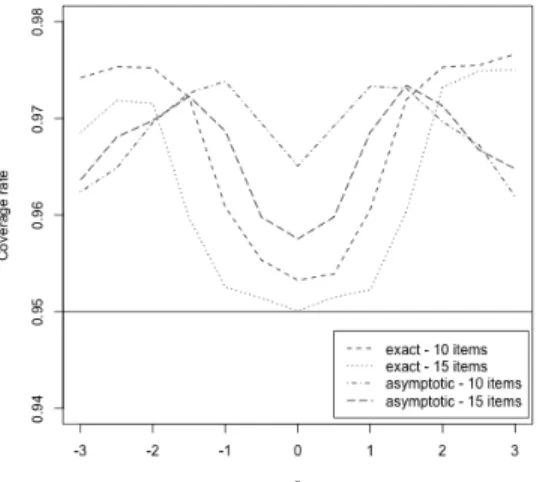
27 Coverage rate of the 95% confidence interval . . . 25

28 Average computing time for an exact p-value . . . 28

29 Average computing time for a confidence interval . . . 29

210 The exact p-values for the LSAT data . . . 30

211 95% confidence intervals for the SF-12 data . . . 31

31 k-lag autocorrelation of two parameters . . . 54

32 Traceplot of two parameters . . . 54

33 Joint posterior density of λ1 and λ13 for Item 20 . . . 58

(8)

41 Prior probabilities P(m|α, N) . . . 73

42 Posterior class sizes under fixed α . . . 77

43 Posterior class sizes with α∼Ga(0.001,100) . . . 78

44 Trace lines for posterior samples of α - black: 3 classes, red: 4 classes . . . 79

45 Mean estimated IRFs in simulation study 1 . . . 83

46 Mean of |pˆj(θ)−pj(θ)| over 28 items in simulation study 1 . . . 84

47 Mean estimated IRFs in simulation study 2 . . . 86

48 Mean of |pˆj(θ)−pj(θ)| over 20 items in simulation study 2 . . . 87

49 Average absolute difference of the estimated IRFs for the ECPE data . . . 88

(9)

List of Tables

21 Average confidence interval lengths . . . 26

22 18 patterns that are rejected under the exact test . . . 36

23 10 patterns that are rejected under the asymptotic approach . . . 36

31 ECPE Bayesian estimates of LCDM item parameters . . . 56

41 ECPE item response probabilities under HDCM . . . 81

42 Summary of the average CR . . . 83

43 Generated item parameters in simulation study 2 . . . 85

(10)

Acknowledgements

Firstly, I want to express my deep gratitude for Dr. Lawrence DeCarlo and Dr. Matthew Johnson, my advisers. I am forever indebted to your patient and careful guidance. I have lost count of how much time you spent advising me. Dr. Johnson, thank you for giving me the freedom and guiding me exploring many research topics. Our discussions are some of my most memorable moments during my graduate school career. Dr. DeCarlo, thank you for always sharing your perspectives. Your passion for psychometrics research encourages me to become a better researcher. I will always look up to my advisers not only as intellectuals but also as persons.

I want to thank other professors whom I had the honor to work with, especially Dr. Young-Sun Lee and Dr. Bryan Keller. Thank you for all the opportunities you brought me and research ideas you shared. I would also like to thank all the colleagues I worked with at EdLab. A special thanks goes to Dr. Gary Natriello and Dr. Hui Soo Chae. I am grateful for your support in all these years. I would not have made this far without your help. I would like to show my appreciations to Dr. Zhiliang Ying for being on my dissertation committee and sharing his insightful and valuable suggestions.

(11)

me and the belief you had in me all these years. Especially, I want to thank my wife, Fei, for accompanying me through this journey.

(12)

(13)

Chapter 1 Introduction

My research interests span the areas of latent variable models, categorical data analysis, and Bayesian methods. A common theme of my research is to understand and improve the theory and applications of psychometric models. To achieve this, I utilize techniques from both frequentist and Bayesian traditions. Specifically, a significant portion of my research deals with the development of computational methods for various psychometric models. Given the rapid improvement of computing power and the emergence of big data, it is certainly an area that will grow more relevant and more important. A wide range of popular psychometric models - item response theory (IRT), cognitive diagnosis models (CDM), latent class models have been covered in my research. Many of them have a Bayesian and computational focus.

(14)

1.1 The First Study: Small Sample Size Confidence

Intervals for IRT

IRT is widely used in educational and psychological testing. One of the core purposes of IRT is to map students’ ability onto a latent continuum. Since only a finite number of items can be administered, abilities are estimated with uncertainty. Traditionally, the standard error of the ability estimator is based on the large sample approximation (i.e., square root of the inverted fisher information). While it might be reasonable for longer tests, in reality, we often have to use short to medium length instruments (e.g., personality tests). The standard errors and the confidence intervals based on the large sample approximation could be highly inaccurate under these circumstances.

To address this important issue, the first study (X. Liu, Han, & Johnson, 2018) pro-posed a framework to construct hypothesis testing based on exact distribution. Confidence intervals of ability estimates are obtained by inverting the hypothesis tests . As a result, the type-I error rate is well controlled under even small to medium test lengths. A major hurdle to this approach is the heavy computational requirements. Instead of permuting all possible response patterns by brute force, I developed a branch and bound algorithm that can calculate p-values efficiently. With the help of the algorithm, the exact distribution approach is now computationally feasible for even medium test lengths. This work is not only technically interesting, but also enables practitioners and researchers to recognize the measurement uncertainty more accurately so that, ultimately, decision making can benefit from the improved measurement practice.

(15)

1.2 The Second Study: MCMC for Log-linear CDM

Models

Bayesian statistics is another major piece of my research. Markov chain Monte Carlo (MCMC) has been widely used to estimate many kinds of psychometric models. Cogni-tive diagnosis models (CDM) is no exception. The second study (X. Liu & Johnson, n.d.) introduced a Gibbs sampler for estimating the saturated log-linear CDM model. By repa-rameterizing the log-linear CDM model, I was able to analytically derive the closed form update steps for the Gibbs sampler. The automatic update steps do not require tunning which makes it easy to use. I also gave the linear transformation that would transform the posterior samples back to the original log-linear CDM parameterization.

The introduced method potentially provides an automatic solution for researchers who may be interested in performing Bayesian analysis in CDM. Even though I introduced the method in the context of the saturated log-linear models, it can be easily extended to other specific CDM models.

1.3 The Third Study: Bayesian Nonparametric

Ordered Latent Class Model

The third study develops Bayesian nonparametric methods for ordered latent class models. In latent class or mixture models, the number of classes usually has to be specified a priori. Essentially, it becomes a modeling choice that is either based on a researcher’s substantive

(16)

Selecting models based on some model fit indices is not always straightforward. Different fit indices might penalize the complexity of the model differently which may result in different conclusions. In addition, in some cases, a researcher might have to fit a large number of models with different number of classes before the optimal model can be determined. Therefore, it may create heavy computational burdens. More importantly, all inferences are conditioned on the selected model. It ignores the uncertainty of the model choice. By assigning stochastic process priors to latent class assignments, Bayesian nonparametrics can fit a model with an infinite number of classes. The posterior distribution of the number of classes provides a better picture of model uncertainty. Unlike the traditional methods, some inferences do not have to be conditioned on one selected model. Instead, marginal quantities can be obtained by averaging over the posterior distribution of the models with different dimensions which can account for the model uncertainty.

(17)

Chapter 2 The UMP Exact Test and the

Confidence Interval for Person

Parameters in IRT Models

2.1 Introduction

In Item Response Theory (IRT), the person parameter is often estimated with the maximum likelihood estimator (MLE) (Hambleton & Swaminathan, 1985). Under large sample sizes, the MLE is approximately normally distributed with asymptotic variance given by the inverse of the Fisher information (Baker & Kim, 2004). Based on the asymptotic normality, one can construct hypothesis tests and confidence intervals for the person parameter (Casella & Berger, 2001). However, the propriety of the asymptotic assumption is questionable under practical situations where the test is often of moderate lengths. As a result, the

(18)

could be very misleading. This problem has been recognized in earlier research (Lord, 1983; Klauer, 1991; Doebler, Doebler, & Holling, 2012; Biehler, Holling, & Doebler, 2014). Thus, developing statistical inference procedures that do not depend on the asymptotic normality is of practical importance. Two approaches are generally discussed.

One approach is to base the inference on the exact distribution of the response patterns. The idea of using the exact distribution of response patterns in IRT was initially introduced for the purpose of assessing response pattern fit (Molenaar & Hoijtink, 1990). Klauer (1991) further derived the uniformly most powerful unbiased (UMPU) test and the uniformly most accurate confidence interval based on the exact distribution of the response patterns in the Rasch model. Klauer noticed that the raw sum score is a sufficient statistic for the person parameter in the Rasch model. Therefore, response patterns in the Rasch model can be reduced to raw sum scores. Furthermore, the test statistic based on the raw sum score was randomized to achieve the level α unbiased test. The computation is tractable as only the exact distribution of the raw sum scores are needed. As the number of items increases, the number of possible raw sum scores increases linearly.

The exact distribution approach has also been extended to the two-parameter logistic (2PL) model. Unfortunately, the raw sum score is no longer a sufficient statistic for the person parameter in the 2PL model. Instead of calculating the exact distribution of the sufficient statistic, the exact distribution for a Wald statistic was calculated (Doebler et al., 2012). And confidence intervals were derived by inverting the exact test. In the same paper, the authors also proposed a hybrid Bayesian approach by incorporating a prior distribution on the person parameter.

(19)

person parameter using a higher-order approximation (Biehler et al., 2014). The saddle-point approximation works well for IRT models within the exponential family and is relatively easy to implement. However, it does not yield the optimal confidence interval such as the uniformly most accurate confidence interval (Klauer, 1991).

Given the much improved computing power, calculating the exact distribution under small to moderate item lengths becomes feasible. In the present work, we extend Klauer’s (1991) approach to the 2PL model. In fact, we generalize the procedure for IRT models in the exponential family. In addition, an efficient branch and bound algorithm is introduced.

2.2 Existing Methods

The small sample inference methods mentioned in the introduction have been rarely dis-cussed in the IRT literature. As a result, readers may not be familiar with them. We will briefly review these ideas in this section.

2.2.1 Saddle-point Approximation

A probability distribution can be completely characterized by its characteristic function (Casella & Berger, 2001). The density function of a distribution can be obtained by inverse-Fourier transformation of the characteristic function. Often, the transformation has to be approximated. The goal of the saddle-point approach here is to provide a robust approxima-tion to the distribuapproxima-tion of the sufficient statistic given an ability parameter, i.e. P (T(X)|θ0),

under small sample size. Biehler et al. (2014) described the approximation in the appendix of their paper. The derivation involves exponential tilting and Edgeworth expansion.

(20)

Com-pared to an error term of O(n−1/2₎ from the first-order normal approximation, the

saddle-point approximation has an error term of O(n−1). Consequently, it converges faster to the true distribution as the number of items increases (Biehler et al., 2014). This desired feature provides a relatively accurate approximation under small sample sizes. The tail probabilities can be obtained through integrating the approximated probability density function. The ap-proximation of this integral is provided by the Lugannani-Rice formula (Lugannani & Rice, 1980). Then inverting two equal tail tests gives the confidence interval.

The approximation depends on the availability of the mean and the variance of the distribution of the sufficient statistic. This is possible for the exponential family as the distribution of the sufficient statistic is also within the same family. The cumulant generating function of the sufficient statistic is known, and its mean and variance are given by the first two cumulants.

This method only works for IRT models within exponential family. Although the ap-proximation is highly accurate, simulations show that the coverage rate of the resulting confidence interval may still fall below the nominal rate for some conditions (Biehler et al., 2014).

2.2.2 Exact Distribution Approaches

The methods proposed in Doebler et al. (2012) are more closely related to our approach in the sense that they are all based on the exact finite sample distribution of the response patterns.

(21)

2.2.2.1 The Hybrid Bayesian Approach

To test the two-sided hypothesis H0 : θ = θ0 versus Ha : θ 6= θ0, Doebler et al. (2012)

proposed a likelihood ratio type statistic in the form of

lθ0(x) = Pf(x) Pθ0(x) , (2.1) where Pf(x) = R

θ6=θ0Pθ(x)f(θ)dθ, Pθ(x) is the probability of the response vector x under

some ability levelθ, andf(θ) is the prior distribution of the person parameter. Intuitively,l in equation 2.1 is a ratio of the weighted average of likelihood over a prior distribution to the likelihood under the hypothesized value θ =θ0. A larger l would provide stronger evidence

to reject θ0. Then the acceptance region can be defined as

A1,θ0 ={x:lθ0(x)≤C}.

The constant C is chosen such that it is the smallest that can satisfy Pθ0(Aθ0)≥1−α for

some nominal level α. Due to discreteness, the nominal level generally cannot be achieved exactly.

The associated confidence set can be obtained by inverting the above test. The idea is to find allθ that will not be rejected given some observed response pattern. So the confidence set is

I1(x) ={θ :x∈A1,θ}. (2.2)

Doebler et al. (2012) showed that the interval in (2.2) minimizes the average expected length, Z

θ

(22)

2.2.2.2 The Exact Normal Approach

The idea of this approach is to construct confidence intervals based on the asymptotic vari-ance of the estimator. Instead of getting probabilities from the asymptotic distribution, the authors calculated probabilities exactly from the finite sample distribution (Doebler et al., 2012). For the same two-sided hypothesis, a Wald-type statistic was proposed,

zθ0(x) = ˆ θ(x)−θ0 r varθˆ(x) , (2.3)

where _θˆ_{is an estimator for} _θ_{. Note that} _θˆ_{does not have to be the MLE. Other estimators} such as weighted likelihood estimator (Warm, 1989) would also work here. Similar to the Hybrid Bayesian approach, the acceptance region is then

A2,θ0 ={|zθ0| ≤C}.

The constant C is the smallest that can satisfy Pθ0(Aθ0)≥1−α for some nominal level α.

The confidence set can be obtained by inverting the test in a similar fashion.

I2(x) ={θ :x∈A2,θ}.

This approach is similar to the standard approach based on asymptotic normality. How-ever, the authors did not state any optimality for this method (Doebler et al., 2012).

2.2.2.3 Limitations

This class of approaches does not rely on approximation of the distribution of a test statistic. Instead, probabilities are calculated based on the exact distribution of response patterns. As a result, the coverage rate of the confidence set will never fall below the nominal level.

(23)

But there are limitations. Due to discreteness, the coverage rate of the confidence set might be higher than the nominal level. In other words, confidence sets from methods based on exact distribution are often conservative. In addition, the Bayesian approach is sensitive to the choice of prior. The exact normal approach does not generally meet any optimality criterion. More importantly, the resulting confidence sets from the above two methods are not necessarilyintervals (Doebler et al., 2012). It is due to the fact that the endpoints of the acceptance region need not be monotone in θ0 (Agresti, 2003). Casella and Berger (2001)

also discussed this problem.

The exact distribution approach using sufficient statistic (Klauer, 1991) avoids this par-ticular problem. Furthermore, it leads to the uniformly most powerful test which is a more common optimality criterion.

2.3 Theory

In this section, we derive the Uniformly Most Powerful (UMP) test for IRT models in the exponential family.

2.3.1 IRT models in the exponential family

Lord (1980) showed that 1PL and 2PL models with known item parameters are in the exponential family. Here, without loss of generality, we demonstrate the result for the 2PL model when the item parameters are known. The item response function for the 2PL model is given by

(24)

where θi is the latent ability of ith subject, aj is the discrimination parameter for jth item,

and bj is the difficulty parameter for jth item. Then for a given response pattern x, the

likelihood function for θ can be written as

L(θ|x) = n Y j=1 Pxj j (1−Pj)1−xj = n Y j=1 exp[aj(θ−bj)] 1−exp[aj(θ−bj)] xj 1 1−exp[aj(θ−bj)] 1−xj . The likelihood in equation 2.3.1 can be further factorized into the following form (for details, see appendix) L(θ|x) = exp[η(θ)T(x)]h(x)g(θ), where exp[η(θ)T(x)] = exp(θ n X j=1 ajxj), h(x) = exp(− n X j=1 ajxjbj), and g(θ) = n Y j=1 {1−exp[aj(θ−bj)]} −1 .

This shows that 2PL model is in the exponential family and θ is a natural parameter. Furthermore, T(x) = Pn

j=1ajxj is a sufficient statistic for θ. Under the 1PL model, the

sufficient statistic reduces to the raw sum score, since the discrimination parameters are constant across items. Furthermore, because η(θ) = θ is an increasing function, 1PL and 2PL models have the monotone likelihood ratio (MLR) property (Casella & Berger, 2001).

(25)

2.3.2 The UMP one-sided hypothesis test

Consider testing H0 :θ ≥θ0 versus H1 :θ < θ0 with a test of the form

φ1 =          1 T(x)< C 0 T(x)≥C, whereT(x) =Pn

j=1ajxj is a sufficient statistic forθ. Ifφ = 1, the test rejects H0. Ifφ = 0,

the test fails to reject H0. The constantC is minimal that can satisfy Pθ0(T(X)< C)≤α,

for some nominal level α. BecauseT(x)is a sufficient statistic for θ and the MLR property holds, by the Karlin-Rubin theorem, the test φ is a UMP level α? = Pθ0(T(X) < C) test

(Casella & Berger, 2001).

In the context of 1PL and 2PL models, the distribution of the sufficient statistic is discrete. Thus, in general, α? cannot achieve the nominal level α. If a size α test is desired, the sufficient statistic can be randomized by adding a random component (Klauer, 1991). However, the randomized statistic leads to randomized decision. In practice, randomized decisions are problematic. For example, two examinees who have the exact same response pattern might receive different decisions. This raises a serious fairness question. In this paper, we do not provide details for randomizing the test.

Instead of calculating the constantC, the exact p-value can also be obtained. For a given observed response pattern x0, the p-value is given by

Pθ0(T(X)≤T(x0)) =

X

x: T(x)≤T(x0)

Pθ0(X =x). (2.4)

For testing H0 : θ ≥ θ0 versus H1 : θ < θ0, we can compare the exact p-value against the

(26)

In this section, we derived the one-sided UMP test for IRT models in the exponential family. Notice that for testing H0 : θ ≤ θ0 versus θ > θ0, the derivation of the UMP test

follow the same approach.

2.3.3 The two-sided test

For testing H0 :θ = θ0 versus H1 : θ 6=θ0, the UMP test does not exist (Casella & Berger,

2001; Klauer, 1991). Klauer (1991) was able to derive the two-sided UMP unbiased test. However, this approach requires a continuous test statistic from randomization. Here, we construct an equal-tail two-sided test with some nominal level α. The test has the following form φ2 =          1 T(x)< C1 orT(x)> C2 0 C2 ≤T(x)≤C1, where T(x) = Pn

j=1ajxj. C1 is maximal such that

Pθ0(T (x)< C1)≤α/2. (2.5)

Similarly, C2 is minimal that satisfies

Pθ0(T (x)> C2)≤α/2. (2.6)

From this definition, one can see that the test is essentially two one-tailed tests with equal significance level α/2. Again, due to discreteness, in general the equal signs in (2.5) and (2.6) cannot be achieved.

(27)

2.3.4 The confidence interval

Inverting the equal tail test φ2 leads to the confidence set. Given an observed response

patternx0, we find all θ that will not be rejected,

I3(x0) ={θ :φ2,x0(θ) = 0}.

Unlike I1 or I2, the endpoints of the acceptance region in this method is monotone in θ0.

This guarantees that the set I3 is an interval. This is also referred to as the tail method

(Agresti, 2003). Consequently, the lower bound of the confidence interval can be obtained by solving

Pθ0(T (X)≤T (x0)) =α/2,

for θ0. Similarly, the solution for

Pθ0(T (X)≥T (x0)) =α/2, (2.7)

gives the upper bound. NowI3 can be expressed as

I3(x0) ={θ :θl ≤θ≤θu}, (2.8)

where θl and θu are solutions of (2.7) and (2.8) as functions of θ, which can be obtained by

standard root finding algorithms.

2.3.5 Computational algorithm

One difficulty associated with the exact distribution approach is the computational complex-ity. For the 1PL model, the computation is manageable. As the number of items increases,

(28)

the number of weighted sum scores, in general, increases exponentially. Therefore, compu-tation by brute force would quickly become too time consuming to be feasible as the test length increases. In this section, we introduce an efficient branch and bound algorithm for calculating exact p-values.

2.3.5.1 Formulation of the problem

By brute force, finding the exact p-value of a given response pattern x0 as defined in (2.4)

requires the complete enumeration of all response patterns. However, it should be noticed that only response patterns that produce sufficient statistics not larger than the sufficient statistic of the observed response pattern need to be considered. Thus, the problem translates to finding all possible response pattern xsuch that

a1x1+a2x2+· · ·+ajxj ≤T(x0). (2.9)

Enumerating subject to a constraint in the form of (2.9) is a discrete mathematical pro-gramming problem that can be solved by the branch and bound algorithm. The algorithm was first conceptualized in 1960 (Land & Doig, 1960), and was later formalized and given its current name for the purpose of solving the well-known traveling salesman problem (Little, Murty, Sweeney, & Karel, 1963).

2.3.5.2 The binary tree representation

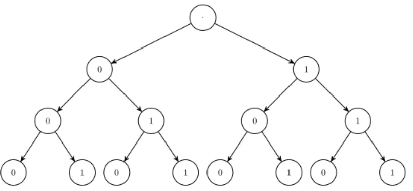
The response patterns can be represented using a binary tree structure. Figure 21 shows an example of three items. Each branch of the tree represents a response pattern. For example, the branch 0 → 0 → 0 represents the response pattern (0,0,0). For J items, there are 2J

(29)

. 0 0 0 1 1 0 1 1 0 0 1 1 0 1

Figure 21: The binary tree representation of response patterns

. 0 0 0 a3 a2 0 a3 a1 0 0 a3 a2 0 a3

Figure 22: The binary tree representation of weighted sum scores

possible response patterns. Thus, the number of the nodes at the bottom of the tree is 2J.

The tree has J+ 1 levels, with (j+ 1)th level representing the response for _jth item.

Each response pattern is associated with a weighted sum score. Therefore, the weighted sum scores can also be represented using the same binary tree structure by multiplying to-gether the dichotomous responses in Figure 21 and the associated discrimination parameters (see Figure 22). Adding the nodes within a branch leads to the weighted sum score for the response pattern presented by the branch. For example, the weighted sum score for the response pattern(1,0,1) is a1+ 0 +a3.

(30)

2.3.5.3 Branch and bound

Because the item discrimination parameters in the 2PL are usually constrained to be positive, the weighted sum score is non-decreasing as we go deeper along any branch in the tree. For a given observed response patternx0, the constraintT(x0) in (2.9) can be computed. Then

we only need to consider those branches that satisfy the constraint.

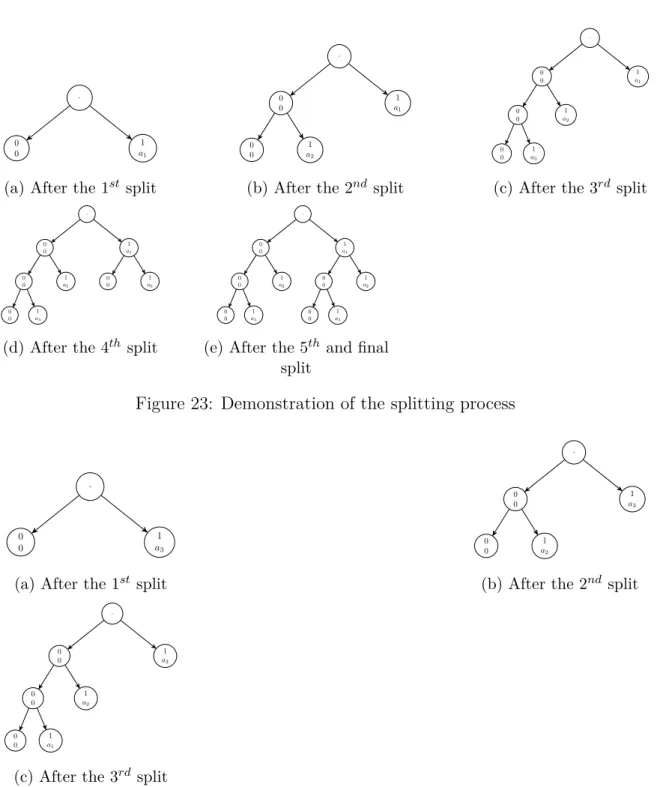
The construction of the binary tree can be viewed as a series of splitting operations. While the constraint is satisfied, the branch keeps splitting. The weighted sum score is checked against the constraint after each splitting. If the constraint is not satisfied, any further splitting could not possibly produce response patterns that could satisfy (2.9) due to the non-decreasingness mentioned above. Thus, the branch can be terminated.

For example, suppose x0 = (1,0,0) and a1 < a2 < a3. The sufficient statistic of the

observed response pattern is then T(x0) = a1. The splitting process is demonstrated in

Figure 23.

Notice that, after the3rdsplit, the branch₀_→₁did not split any further as the weighted

sum is 0 +a2 > a1. After the final split, all the response patterns that could potentially

satisfy the constraint (2.9) should have reached the bottom of the tree. Out of the four branches reached the bottom, only 0→0→0 and 1→0→0satisfy (2.9). Thus the exact p-value is

Pθ0(T(X)≤T(x0)) = Pθ0{X = (000)}+Pθ0{X = (100)}. (2.10)

Instead of calculating probabilities for all eight possible patterns, only two probabilities need to be evaluated using the branch and bound algorithm.

(31)

descend-.

0 0

1 a1

(a) After the1st split

. 0 0 0 0 1 a2 1 a1

(b) After the2nd split

. 0 0 0 0 0 0 1 a3 1 a2 1 a1

(c) After the3rd split

. 0 0 0 0 0 0 1 a3 1 a2 1 a1 0 0 1 a2

(d) After the 4th split

. 0 0 0 0 0 0 1 a3 1 a2 1 a1 0 0 0 0 1 a3 1 a2

(e) After the5th and final

split

Figure 23: Demonstration of the splitting process

.

0 0

1

a3

(a) After the1st split

. 0 0 0 0 1 a2 1 a3

(b) After the 2nd split

. 0 0 0 0 0 0 1 a1 1 a2 1 a3

(c) After the 3rd split

Figure 24: The splitting process for ranked items

ing order according to their discrimination parameters before constructing the tree. For the same example above, the splitting process after ranking is demonstrated in Figure 24. Compared to the five splits in Figure 23, it only needs three splits after ranking the items.

(32)

However, we should take the computational cost of ranking into our consideration. But in our experience, the cost of ranking is negligible compared to the improved efficiency in the branch and bound algorithm.

In the example we provided, the tree is always traversed as deep as possible along a branch before exploring parallel branches. This is called the Depth First Search(DFS) (Leiserson, Rivest, Stein, & Cormen, 2009). We implemented this version of the branch and bound algorithm for calculating exact p-values. We also used Brent’s algorithm (Brent, 1973) to find bounds for the confidence interval. The C++ code is available from the first author.

2.4 Simulation Study

2.4.1 Type-I error and power of the one-tail test

A simulation study was conducted to examine the type-I error rate and the power of the proposed exact test for the 2PL model under different conditions. The difficulty with such a simulation study is that the power of the test is associated with many different factors. The number of items is expected to affect the power. Also, for a given set of items, the power is likely to vary for different ability levels. Moreover, the power depends on the difference between the tested ability level and the true ability level, i.e.

∆θ =θ0−θ. (2.11)

However, the most difficult part is perhaps that different sets of item parameters would likely to have different power curves. Considering this, we decided to investigate the average power for item parameters from their usual distributions under different conditions.

(33)

2.4.1.1 Design

Four test lengths were considered: J = 5,10,15, and 20 items. For each test length, seven effect sizes as defined in Equation 2.11 were examined, ∆θ = 0,0.5,1.0, . . . ,3.0. Moreover, twenty-five hypothesized ability level θ0s were selected from −3 to 3 by intervals of 0.25.

Then the true ability level θs were computed by θ =θ0−∆θ.

Given a pair ofJ and ∆θ, item difficulty parametersbj and item discrimination

param-eters aj, were randomly generated from uniform distributions, U(−2.0,2.0) and U(0.5,2.0)

respectively. At each θ, a response pattern x0 was randomly generated using item

param-eters a and b under the 2PL model. Then we test the one-sided hypothesis H0 : θ ≥ θ0

against H1 : θ < θ0. The exact p-value was calculated as in (2.4) using the branch and

bound algorithm. H0 is rejected if the p-value is less than α= 0.05.

For each combination of the length J and the effect size ∆θ, the above process was replicated 50,000 times.

2.4.1.2 Results

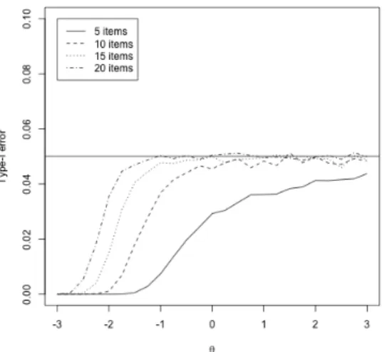
Figure 25 shows the average type-I error rate (∆θ = 0) under different item lengths. When there are onlyJ = 5 items, the type-I error rate is significantly lower than the nominal level α = 0.05. This is due to the discreteness of the response patterns. For 5 items, there are 25 = 32 possible response patterns. However, as the number of items increases, the number of possible response patterns increases exponentially. As a result, the type-I error rate is getting very close to the nominal level for moderate and high θ0 when item length increases

(34)

Figure 25: The type-I error rate from the simulation

extreme negative value. For a given set of items, the response pattern x= (0,0, . . . ,0)has the weighted sum score PJ

j=1ajxj = 0 which is the smallest among all possible response

patterns. If θ0 is so small that Pθ0(X = (0,0, . . . ,0)) > α, the test will not reject θ0 given

any observed response pattern at the nominal level α. As we pointed out earlier, if the nominal level is desired, the decision has to be randomized.

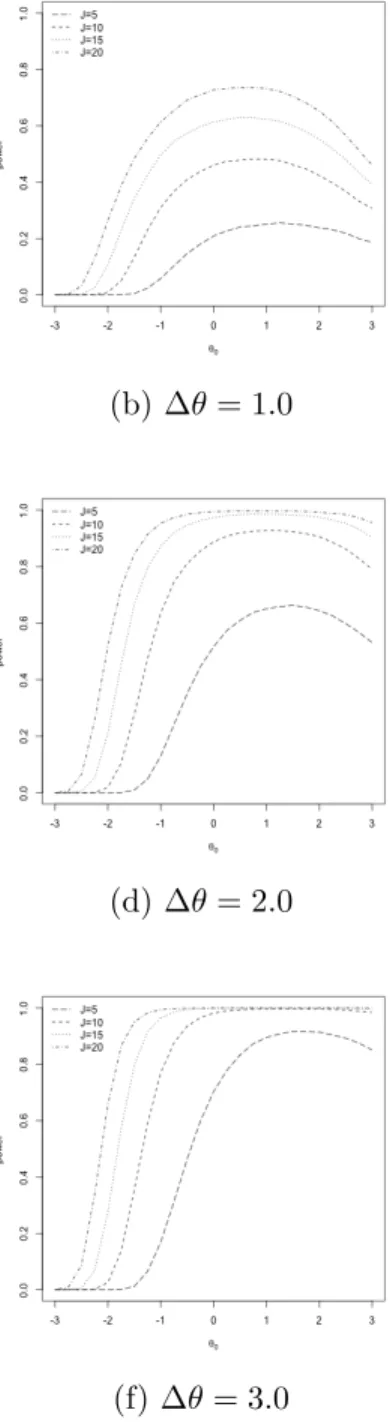
The power curves for ∆θ = 0.5,1.0, . . . ,3.0, are shown in Figure 26. Power is highest for null values of ability, θ0, in the middle part of the scale. Power drops as the null value,

θ0, moves towards the two extremes. The shape of the power curve is likely due to the way

we generated the item parameters, which produced a test information curve that is highest near zero on the ability scale.

As expected, the power increases as the number of items increases. The power also increases with∆θ. For a five item instrument, the power is quite low across all ability levels except for very large ∆θ. Meanwhile, for the item length J = 20, the power is reasonably good around medium level θ0. When ∆θ = 0.5, the power is low, even for a twenty item

(35)

Figure 26: Statistical power under different conditions

(a)∆θ= 0.5 (b)∆θ= 1.0

(c) ∆θ= 1.5 (d)∆θ= 2.0

(36)

instrument.

2.4.2 Coverage rate of the confidence interval

2.4.2.1 Design

To examine the coverage rate of the proposed confidence interval, we conducted the second simulation study. Item discrimination parameters and difficulty parameters were generated from the same uniform distributions in the first simulation. We considered 13 ability pa-rameters from −3 to +3 by intervals of 0.5. Response patterns were generated from the 2PL model. For each generated response pattern, the bounds of the 95% confidence interval were obtained by solving (2.7) and (2.8). In the case of extreme patterns, the bounds were limited to−5and +5. Two item lengths were considered: 10and15. The process replicated 50,000 times for each condition.

We also calculated confidence intervals based on the standard asymptotic approach and examined the coverage rates for comparison. For the 2PL model, the Fisher information is given by ω(ˆθ) = J X j=1 a2 jexp(−aj(ˆθ−bj)) [1 + exp(−aj(ˆθ−bj))]2 , (2.12)

where _θˆ_{is the MLE of the person parameter. The asymptotic standard error then can be} obtained by taking square root of the inverted Fisher information, i.e. S.E.= q1

ω(ˆθ) (Baker

(37)

Figure 27: Coverage rate of the 95% confidence interval

2.4.2.2 Results

Figure 27 shows the coverage rate of the 95% confidence interval for different test lengths. As expected from the exact approach, the coverage rate does not fall below the nominal level for the entire range of ability parameter θ. When θ is close to 0, the coverage rate is very close to the nominal level. As the it goes towards extreme, the coverage rate is getting higher. Agresti (2003) noted this problem in the context of binomial proportions. When θ is sufficiently low, the interval can never excludeθ by falling below it. In this case, the lower bound on the coverage rate is actually1−α/2rather than1−α. The other direction follows the same rationale. that being said, the coverage rate never exceeds98% in our simulations even for extreme person parameters. More items would lead to a “less discrete” test statistic under the 2PL model. Consequently, the coverage rate is closer to the nominal level. For a test with 15 items, the coverage rate is very close to 95% for a good range of θ, and almost exact for medium levelθ. On the other hand, the confidence intervals based on the standard asymptotic approach are overly conservative. Even with 15 items, the coverage rate is still

(38)

not close to the nominal level for medium levelθ.

2.4.3 Lengths of the confidence interval

2.4.3.1 Design

The purpose of this simulation study is to examine the lengths of the proposed confidence interval for different levels of generating person parameter. We also compared the results with the standard confidence interval based on the asymptotic normality of the MLE. We considered 5 ability parameters, i.e. θ = −3.0,−2.0, . . . ,3.0. For each θ, we generated 10000 responses from the 2PL model. Item parameters were treated as random effects and generated in the same fashion as in the previous simulations. Average length of the confidence intervals are computed for both the exact approach and the standard asymptotic approach.

2.4.3.2 Results

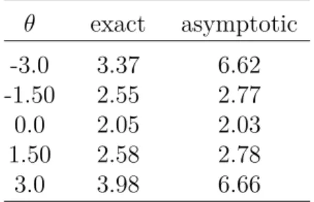
Table 21: Average confidence interval lengths

(a)10 items θ exact asymptotic -3.0 3.83 9.62 -1.50 3.16 4.17 0.0 2.60 2.58 1.50 3.30 4.17 3.0 4.58 9.55 (b)15 items θ exact asymptotic -3.0 3.37 6.62 -1.50 2.55 2.77 0.0 2.05 2.03 1.50 2.58 2.78 3.0 3.98 6.66

Table 21 shows average confidence interval lengths for both the exact distribution ap-proach and the standard asymptotic apap-proach under 10 items and 15 items. While main-taining adequate coverage rates as demonstrated in the previous simulation, the exact

(39)

dis-tribution approach results in shorter confidence intervals across different ability levels. The difference is smaller in the middle of the ability level. The average lengths of the proposed confidence interval are comparable to those reported in Doebler et al. (2012) in the medium θ level, but shorter for more extreme θ values.

2.4.4 Computational time

2.4.4.1 Design

In order to investigate the feasibility of our proposed method, we benchmarked computa-tional time required. Six test lengths were considered - 5, 10, 15, 20, 25, and 30. Item parameters were generated from the same uniform distributions used in the other two simu-lations. Person parameters were generated from a standard normal distribution. Response patterns were generated under 2PL model. For the problem of testing the one-sided hypoth-esis H0 : θ ≥ 1.2 versus H1 : θ < 1.2, the time required to compute an exact p-value was

recorded. We ran 100 replications, and the average time was taken. We also benchmarked efficiency of finding confidence intervals for various test lengths.

2.4.4.2 Results

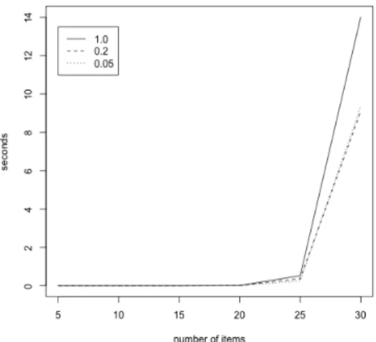
The average number of seconds required for computing exact p-values are in Figure 28. The p-values are calculated up to the specified thresholds - 1.0, 0.2, and 0.05. When the test length is not greater than 25, it takes well less than 1 second to compute an exact p-value. The time difference between different threshold is minimal. When the test length is 30, the computational cost becomes significantly higher. Now, computing an exact p-value takes

(40)

Figure 28: Average computing time for an exact p-value

about 14 seconds. If we are content with a threshold of0.2or0.05, the average time needed would be roughly 9 seconds.

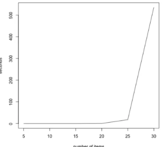
The average time required for computing a confidence interval under different test lengths are in Figure 29. Computing the confidence interval for a response pattern with no more than 20 items is very fast and takes less than 1 second. But for a 25-item pattern, it would take 18 seconds on average. When the test length is 30, the average computing time quickly increases to about 540 seconds.

2.5 Real data example

2.5.1 Hypothesis testing for LSAT data

In this section, we demonstrate a practical application of the proposed method. Dichoto-mous responses to 5questions from1000individuals were extracted from the Rpackageltm (Rizopoulos, 2006). The data set is from the Law School Admission Test(LSAT) (Bock &

(41)

Figure 29: Average computing time for a confidence interval

Lieberman, 1970).

In this example, we fit the Rasch model to the data. The difficulty parameters, βj, j =

1,2, . . . ,5, are estimated through conditional maximum likelihood estimation using the R package eRm (Mair & Hatzinger, 2007). For identification purposes, we constrained the parameters so thatP5

i=1βj = 0. The estimated parameters are then treated as known.

We are interested in testing the one-sided hypothesisH0 :θ≥1.28againstH1 :θ < 1.28.

Under the Rasch model, the sufficient statistic for the ability parameter is the raw sum score. Therefore, 25 _{= 32} possible response patterns can be reduced to ₆ raw sum scores.

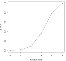
The exact p-value for each raw sum score is calculated and presented in Figure 210. If the nominal level is set at α = 0.05, H0 will be rejected when the raw sum score is 0 or 1. For

(42)

Figure 210: The exact p-values for the LSAT data

2.5.2 Confidence interval for the SF-12 data

The 12-item Short-Form Health Survey (SF-12) is perhaps one of the most widely used patient-reported heath outcome rating scales (J. E. J. Ware & Sherbourne, 1992; J. E. Ware, Kosinski, & Keller, 1996). Hagell and Westergren (2011) analyzed a data set of 150 Parkin-son’s disease patients responding to the SF-12 survey. The original SF-12 survey has 4 dichotomous items and 8 polytomous items. The authors (Hagell & Westergren, 2011) examined thresholds between adjacent response categories for the ploytomous items and decided there were too many categories. They proceeded to dichotomize item responses by collapsing adjacent categories and fitted the Rasch model. A reasonably good fit was reported.

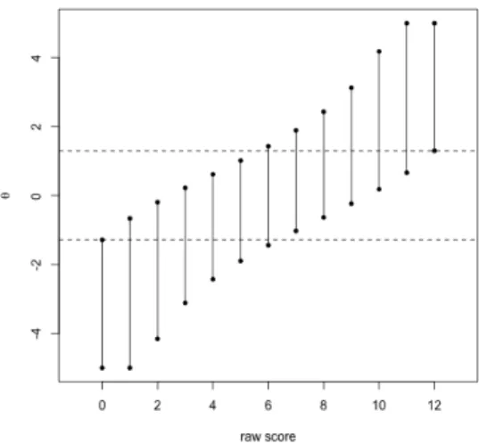
One of the concerns of using short test forms is whether there is enough information to reliably distinguish subjects. Based on the parameter estimates obtained for the Rasch model (see Table 4 in Hagell & Westergren, 2011), we computed confidence intervals for each raw sum score (see Figure 211). In order to be significantly different from the lowest

(43)

Figure 211: 95% confidence intervals for the SF-12 data

score, a person has to obtain a raw score that is at least 7. Similarly, only raw scores less than 6 can be distinguished from the highest score at the nominal level. If a person scored 6 in the survey, there would not be enough evidence to distinguish this individual from any other person.

2.5.3 Hypothesis testing for the food security data

The 10 item food security data were extracted from the 2002 Current Population Survey and analyzed using IRT models (Johnson, 2004). The responses of 9804 individuals were used approximate the posterior distribution of the model parameters for both the Rasch and the 2PL models. The discrimination parameters varied significant. As a result, the Rasch model did not provide an adequate fit and 2PL model was favored. A cutoff score (1.93) was determined so that 95% of food insecure population with latent score greater than 1.93 will respond affirmatively to at least six of the food security items under the IRT model. For details of finding the cutoff score, please refer to Johnson (2004).

(44)

Based on the 2PL item parameters reported (see Table 1 in Johnson, 2004), we calculated exact p-values for the one-sided hypothesis H0 : θ ≤ 1.93 against H1 : θ ≥ 1.93. Of the

possible210_{= 1024}patterns, 18 are rejected at the_α _{= 0.05}level (see Table 22 in Appendix

B). Among them, 1 pattern has a raw score of 10, 10 patterns have raw scores of a 9, and the other 7 patterns have raw scores of 8.

We also calculated p-values based on the asymptotic distribution of standard errors. It results in only 10 patterns being rejected (see Table 23 in Appendix B). For the pattern with a raw score of 10, the MLE of the person parameter is not an interior point. So that pattern is excluded. Out of the 10 patterns with raw scores of 9, only 9 of them were rejected. It also rejects one pattern with a raw score of 8.

In this example, the exact test rejects more patterns compared to the asymptotic ap-proach (Table 23 is a subset of Table 22). Some response patterns that are rejected under the exact test are failed to be rejected using the asymptotic approach. In practice, it would make a difference in decision making for those individuals with these response patterns.

2.6 Discussion

Being able to accurately recognize low reliabilities associated with short test forms is very important. Under the IRT framework, reliability is reflected as information or precision of the estimated latent abilities. Typically, the asymptotic distribution of the MLE is used to recognize the uncertainty of the person parameter estimates. However, the actual distribu-tion is not normal even with 30 items for the 2PL model (Biehler et al., 2014). Developing a method that can obtain an accurate measure of the precision is of practical importance.

(45)

In this paper, we generalized the exact distribution approach for constructing the UMP test, equal-tail two sided test, and the associated confidence interval to IRT models within the exponential family. In addition, we proposed a branch and bound algorithm for the purpose of calculating the exact p-value.

Thissen (2016) argued that instead of reporting score in a yes-or-no fashion regarding a student’s proficiency, we should report proficiency probabilistically. The method we proposed in this paper doesnot provide the probability of a student being proficient given a test score, which should be answered by using Bayesian posterior probabilities (Gelman et al., 2013). However, the exact p-value does provide evidence against the hypothesis that the student is proficient. The discussion of the interpretation of p-values dates back to Fisher (1935). Wasserman (2004) also gave the guidelines: > .05being no evidence,.01−.05being positive evidence, .001-.01 being substantive evidence, and < .001 being decisive evidence against H0.

The branch and bound algorithm introduced in this paper can be used to compute the exact p-value efficiently. If only the decision of whether to reject H0 at the nominal level α

is desired and the exact p-value is not of interest, the algorithm can be modified such that it terminates once the α level is reached. As a result, the algorithm could be even more efficient.

There has been some effort in exploring fast algorithms for the response pattern enu-meration. One example is a network algorithm for computing person fit statistic under the Rasch model (Liou & Chang, 1992). The network algorithm uses a directed acyclic graph to represent response patterns. It deals with the enumeration of response patterns conditioned

(46)

ble response patterns given a sufficient statistic constraint. The branch and bound algorithm developed in this paper tackles this problem by using a binary tree structure. Computing exact distributions of the person parameter shares a lot of similarities with computing ex-act distributions of the log-likelihood based person fit statistics (e.g. lz statistic). In the

latter case, there are two main differences. Instead of the hypothesized person parameter value, the computation of the person fit statistics should be conditioned on the estimated person parameter for the observed response pattern. Another major difference is the way how ”extremity” of a pattern is defined. Compared to finding all patterns with greater (or smaller) weighted sum scores, calculating the exact distribution of the person fit statistics requires finding all patterns with worse fit (e.g. smaller log-likelihood). The branch and bound algorithm developed in this paper may be adapted for this task.

As mentioned, the introduced procedure for constructing the UMP test only works for IRT models within the exponential family where a sufficient statistic for the ability parameter exists and the monotone likelihood ratio property holds. It should be noted that the 3PL model is not in the exponential family. Thus, the method does not generalize to the 3PL model or any other model outside the exponential family. The same problem exists for the higher order approximation approach. The saddle-point approximation works only for the exponential family as well (Biehler et al., 2014). Developing appropriate inference procedures and efficient computational algorithms for the 3PL under small sample size still remains a challenge.

(47)

Appendix A

Under the 2PL model, the probability of a correct response for jth item from a subject is Pj(Xj = 1|aj, bj, θ) =

exp[aj(θ−bj)]

1 + exp[aj(θ−bj)]

, (2.13)

where aj is the item discrimination parameter, bj is the item difficulty parameter, and θ is

the ability parameter for the subject. It follows that the likelihood of θ given a response patternX =x is L(θ|x,a,b) = J Y j=1 Pj(Xj = 1|aj, bj, θ)xjPj(Xj = 0|aj, bj, θ)1−xj (2.14) = J Y j=1 { exp[aj(θ−bj)] 1 + exp[aj(θ−bj)] }xj_{ 1 1 + exp[aj(θ−bj)] }1−xj (2.15) = J Y j=1 {exp[aj(θ−bj)]}xj 1 + exp[aj(θ−bj)] { 1 1 + exp[aj(θ−bj)] }xj−xj (2.16) = J Y j=1 {exp[aj(θ−bj)]}xj 1 + exp[aj(θ−bj)] (2.17) = exp[ PJ j=1xjaj(θ−bj)] QJ j=1{1 + exp[aj(θ−bj)]} (2.18) = exp[θ PJ j=1ajxj] exp[PJ j=1ajxjbj] QJ j=1{1 + exp[aj(θ−bj)]} (2.19) = exp[θ J X j=1 ajxj]{exp[ J X j=1 ajxjbj]}−1{ J Y j=1 {1 + exp[aj(θ−bj)]}}−1. (2.20)

The equation 2.20 is in the exponential form L(θ|x) = exp[η(θ)T(x)]h(x)g(θ), where exp[η(θ)T(x)] = exp(θ n X j=1 ajxj), (2.21) h(x) = exp( n X j=1 ajxjbj)−1, (2.22) and g(θ) = n Y {1−exp[a (θ−b )]}−1_. (2.23)

(48)

Appendix B

In the food security data example, we are interested in testing the one-sided hypothesis: H0 : θ ≤ 1.93against H1 :θ ≥1.93. Using the exact test approach, the following response

patterns are rejected at α= 0.05 level:

Table 22: 18 patterns that are rejected under the exact test

0 1 0 1 1 1 1 1 1 1 0 1 1 1 1 1 1 1 1 0 0 1 1 1 1 1 1 1 1 1 1 0 0 1 1 1 1 1 1 1 1 0 1 1 1 1 1 1 1 1 1 1 0 0 1 1 1 1 1 1 1 1 0 1 0 1 1 1 1 1 1 1 0 1 1 1 1 1 1 0 1 1 0 1 1 1 1 1 1 1 1 1 1 0 1 1 1 1 1 1 1 1 1 1 0 1 1 1 1 0 1 1 1 1 0 1 1 1 1 1 1 1 1 1 1 0 1 1 1 1 1 1 1 1 1 1 0 1 1 1 1 1 1 1 1 1 1 0 1 1 1 1 1 1 1 1 1 1 0 1 1 1 1 1 1 1 1 1 1 0 1 1 1 1 1 1 1 1 1 1

Table 23: 10 patterns that are rejected under the asymptotic approach

0 1 1 1 1 1 1 1 1 1 1 0 1 1 1 1 1 1 1 1 1 1 0 1 1 1 1 1 1 0 1 1 0 1 1 1 1 1 1 1 1 1 1 0 1 1 1 1 1 1 1 1 1 1 0 1 1 1 1 1 1 1 1 1 1 0 1 1 1 1 1 1 1 1 1 1 1 0 1 1 1 1 1 1 1 1 1 1 0 1 1 1 1 1 1 1 1 1 1 0

(49)

Chapter 3 Estimating CDMs Using MCMC

3.1 Introduction

In the past two decades, Markov chain Monte Carlo (MCMC) techniques have been widely used for the Bayesian estimation of psychometric models. Not only an alternative to other estimation methods, MCMC algorithms and general purpose MCMC software has been facilitating the development of modern psychometric models that are otherwise difficult to fit (Levy, 2009). In this chapter, we provide a brief survey of MCMC methods used in estimating Cognitive Diagnostic Models (CDM). In addition, a Gibbs sampler for fitting the saturated Log-linear CDM model (LCDM, Henson, Templin, & Willse, 2009) is introduced. The utility of Bayesian inference is demonstrated by analyzing the Examination for the Certificate of Proficiency in English (ECPE) dataset.

To help understand the motivation of developing MCMC methods, consider the following general statistical inference problem. Given a set of observed dataX =x, we would like to

(50)

Under the Bayesian framework, a prior is assigned to the parameters, i.e. p(θ). Then we are interested in the posterior distribution of the model parameters given the observed data, i.e.

p(θ|x) = R p(x|θ)p(θ)

p(x|θ)p(θ)dθ. (3.1)

In some cases the closed form of the posterior distribution p(θ|x) can be analytically de-rived. However, under other circumstances, the posterior distribution must be approxi-mated numerically. Difficulty arises from the numerical evaluation of the integral in the denominator of (3.1). If θ is unidimensional, the integral can be approximated by

us-ing k quadrature points fairly efficiently. But in general, evaluating the multiple integral R R

· · ·R

p(x|θ)p(θ)dθ1dθ2· · ·dθd requires a high-dimensional grid of kd points in Rd. As the

number of dimensions d grows, integration by quadrature quickly becomes infeasible. This problem is also referred to as the ”curse of dimensionality”. Instead of deterministically evaluating the high-dimensional integral, MCMC algorithms stochastically sample from the posterior distribution by constructing a Markov chain whose stationary distribution is the target posterior distribution. For a detailed review of MCMC, refer to Gelman et al. (2013), Neal (1998), and Brooks, Gelman, Jones, and Meng (2011).

Despite its importance to Bayesian inference, it should be noted that MCMC methods are not limited to Bayesian applications. High-dimensional integrals also arise from com-puting marginal maximum likelihood estimates in some models. As a result, MCMC as a class of efficient stochastic numerical integration algorithms is also used in frequentist applications. In fact, such applications have been developed in psychometrics. For exam-ple, Cai (2010) adapted the Metropolis-Hastings Robbins-Monro algorithm to estimate the high-dimensional item factor analysis model by marginal maximum likelihood. Given much

(51)

improved computing power and the availability of general purpose Bayesian inference soft-ware, the CDM literature, flourishing in relatively recent years, also saw a wide range of applications of MCMC methods.

3.2 MCMC Background

In this section, we provide a brief background and intuition of MCMC for readers who might not be familiar with the concept. A Markov chain is a series of random variables,

Θ(0),Θ(1), . . . ,Θ(t),Θ(t+1), . . ., where the state at time t+ 1depends only on the immediate previous state at t. In other words, the distribution of θ(t+1) is independent of everything

else given Θ(t) ₌_θ(t), i.e.

P(θ(t+1)|θ(0),θ(1), . . . ,θ(t)) =P(θ(t+1)|θ(t)). (3.2) This is often referred to as the Markov property. Additionally, the state space, that is the range of θ, is common across all time points. In practice, it implies the parameter space

of the model cannot be changed. However, there exist MCMC methods that can handle models with variable parameter space - for example, the reversible jump MCMC. This topic is significantly more advanced and out of the scope of this chapter. Interested readers may refer to P. J. Green (1995). Observing the aforementioned Markov property, it is clear that, in order to define a Markov chain, we need to specify the probability of an initial state θ - p0(θ) = P(θ(0) = θ) and the transition probabilities between consecutive states

(52)

t+ 1 can be determined by pt+1(θ) = X ˜ θ pt( ˜θ)Tt( ˜θ,θ). (3.3)

For homogeneous Markov chains, the transition probabilities stay the same across all time points, i.e. Tt(θ,θ0) = T(θ,θ0),∀t. A Markov chain is said to have reached its stationary

or invariant distribution - π(θ) if the distribution of θ does not change according to time

points t any more. Specifically, there exists some t˜such that p˜_t(θ) =π(θ) and

π(θ) = X

˜ θ

π(θ)Tt( ˜θ,θ),∀t≥˜t. (3.4)

The purpose of using MCMC in Bayesian inference is to help us sample from an otherwise difficult posterior distribution. To achieve this goal, we are interested in constructing a Markov chain where the target posterior distribution is invariant. Often, we choose reversible homogeneous Markov chains in which the probability of a transition from the stateθ to the

state θ0 is the same as the probability of a transition from θ0 to θ under the distribution of

states π. Equivalently,

π(θ)T(θ,θ0) = π(θ0)T(θ0,θ). (3.5) The above condition is usually called detailed balance. It is straightforward to show that detailed balance implies invariance, i.e.

X θ0 π(θ0)T(θ0,θ) = X θ0 π(θ)T(θ,θ0) = π(θ)X θ0 T(θ,θ0) = π(θ). (3.6) It should be noted that detailed balance is a sufficent but not necessary condition for a distribution to be invariant (Neal, 1998).

Detailed balance ensures that once a Markov chain reaches its invariant distribution, subsequent states are samples from this invariant distribution. However, we generally do

(53)

not know this invariant distribution which is the target posterior distribution. Instead, we hope the distribution of states at timetconverges in distribution to its invariant distribution π as t → ∞ regardless of its initial probability distribution of states p0(θ). The Markov

chain is ergodic if it holds this property. For a homogeneous Markov chain with an invariant distribution π, it is ergodic if the chain can traverse the entire support of π, i.e.

v = min

θ θ0_:min_π_(θ0₎_>₀T(θ,θ

0

)/π(θ0)>0. (3.7)

For a proof of this theorem, readers can refer to Neal (1998).

The simplest MCMC algorithm is perhaps the Gibbs sampler (Geman & Geman, 1984; Gelfand & Smith, 1990). Suppose we are interested in sampling from a joint distribution given byp(θ1, θ2, . . . , θK)which is our target posterior distribution. Gibbs sampler works by

repeatedly sampling each θk from their full conditional distributions. At the tth iteration,

we

• sample θ(₁t) according to the distribution given by p(θ₁(t)|θ₂(t−1), θ(₃t−1), . . . , θ(_Kt−1)); • sample θ(₂t) according to the distribution given by p(θ(₂t)|θ₁(t), θ₃(t−1), . . . , θ(_Kt−1));

...

• sample θ(_Kt) according to the distribution given by p(θ_K(t)|θ₁(t), θ₂(t), . . . , θ(_Kt)₋₁).

The above steps together form a transition of state fromθt−1 toθtwith probabilitiesT(θ,θ0) that leaves the target distribution invariant. Starting from an initial state θ(0), after

simu-lating the Markov chain long enough, subsequent draws of θ(t) are treated as samples from

(54)

3.3 Applications of MCMC in CDM

Similar to other types of psychometric modeling, instances of applications of MCMC in CDM are numerous. By no means the brief survey in this section is exhaustive, but rather to give readers flavors of the existing literature. The applications of MCMC in CDM can be traced back to earlier papers on the topic. In Junker and Sijtsma (2001), one of the earlier papers on CDM, the authors fit the deterministic inputs, noisy ”and” gate (DINA) model and the noisy inputs, deterministic ”and” gate (NIDA) model using the BUGS (Bayesian inference Using Gibbs Sampling) software (Thomas, Spiegelhalter, & Gilks, 1992).

While de la Torre (2008) provides a reference work for estimating the DINA model by marginal maximum likelihood using the expectation-maximization (EM; Dempster, Laird, & Rubin, 1977) algorithm; the development of the EM algorithm for the higher-order DINA (DINA) model is not trivial. As a result, in de la Torre and Douglas (2004), the HO-DINA model is estimated by a blocked Gibbs sampler (Geman & Geman, 1984; Gelfand & Smith, 1990; Gelman et al., 2013). The full-conditional distributions for HO-DINA do not have closed forms and are not easy to sample from directly. Therefore, the authors adopted the Metropolis algorithm (Metropolis, Rosenbluth, Rosenbluth, Teller, & Teller, 1953; Hastings, 1970). Instead of directly sampling from the full-conditional distributions, at each iteration, the Metropolis algorithm draws a proposed sample value or vector from a proposal distribution (usually a Gaussian distribution), and accepts or rejects it with an ap-propriately defined acceptance probability. To calculate the acceptance probability, only the unnormalized full conditional density function is required. This circumvents the difficulty of obtaining the normalizing constant when it cannot be derived analytically. The combination

(55)

of Gibbs sampler and Metropolis algorithm is usually referred to as the Metropolis-within-Gibbs which is implemented in many general purpose Bayesian inference softwares (e.g. OpenBUGS;Lunn, Spiegelhalter, Thomas, & Best, 2009, JAGS;Plummer, 2005).

One difficulty of using the Metropolis algorithm is the tuning of the sampler. If the variance of the proposal distribution is large, the proposed sample is more likely to be further away from the current sample, which leads to low acceptance probabilities. Consequently, a large number of proposed samples are rejected before an acceptance, and the sampler rarely moves. On the other hand, small variance of the proposal distribution leads to high acceptance probabilities. But the proposed samples tend to be close to the current ones. As a result, the sampler moves slowly and does not explore the posterior distribution very efficiently. Therefore tuning is required so that the Markov chain is mixing at an optimal rate (Roberts, Gelman, & Gilks, 1997). Tuning a sampler could be a tedious task. Culpepper (2015) derived the closed forms of full-conditional distributions for DINA model so that the parameters can be directly sampled without using the Metropolis algorithm. In the same paper, the author also shows that the monotonicity assumption of the DINA model can be enforced by sampling the item parameters from a truncated bi-variate Beta distribution.

In the applications discussed so far, the Q-matrix (Tatsuoka, 1983) needs to be specified before the model can be estimated. In reality, the specification of the Q-matrix is not always straightforward and elements of the Q-matrix can be uncertain. Recognizing this limitation, DeCarlo (2012) proposed a Bayesian model to handle the uncertainty. Instead of treating all elements of the Q-matrix as fixed, the author specifies some of them as Bernoulli distributed random parameters, and assigns a Beta prior to the Bernoulli probabilities. The uncertain

(56)

Bugs software (Spiegelhalter, Thomas, Best, & Lunn, 2014) is used to estimate the model under the reparameterized DINA (RDINA;DeCarlo, 2012) model. DeCarlo and Kinghorn (2016) extend the approach to the case where none of the Q-matrix elements is fixed.

Furthermore, there has also been some other effort developing exploratory Bayesian meth-ods for estimating CDM models without any prior knowledge of the Q-matrix except for the dimensions. Chung (2014) derives a Gibbs sampler for the DINA model and a Metropolis-within-Gibbs algorithm for the rRUM(reduced reparameterized unified model; Hartz, 2002) that include all elements of the Q-matrix as model parameters. The distribution of the attribute patterns for examinees is modeled by a saturated categorical distribution, and the probabilities of the categories are given a Dirichlet prior. Thanks to the categorical-Dirichlet conjugacy, the probabilities of attribute patterns can be directly sampled from Dirichlet pos-terior distributions. By using a saturated categorical distribution, the author did not assume a particular factorization of the joint distribution of the attributes. Correlated attributes with different structures can be modeled in addition to independent attributes. However, the trade-off is the large number of parameters needs to be estimated. For a Q-matrix with K attributes, there are 2K−1 probabilities for the attribute patterns. The Q-matrix is es-timated similarly by using a categorical distribution. Item parameters for the DINA model can be sampled from truncated Beta distributions respecting the monotonicity assumption. Unfortunately, the full-conditional distributions of the item parameters for the rRUM model do not have closed forms. Thus, the Metropolis algorithm is used. Another example of the exploratory Bayesian approach can be found in Chen, Culpepper, Chen, and Douglas (2018). The paper deals with the same problem of estimating the DINA model without knowing the elements of the Q-matrix. Building on the development in understanding the identifiablity

(57)

of the DINA model (Chen, Liu, Xu, & Ying, 2015; J. Liu, Xu, & Ying, 2012, 2013; Xu & Zhang, 2016), Chen et al. (2018) constrain the Q-matrix to be identified in their estimation procedure.

MCMC also aids the development and applications of more complex CDM models. For example, Li, Cohen, Bottge, and Templin (2016) introduce a longitudinal model that incor-porates learning into CDM models. The attribute patterns for each student can change over time. It is modeled by a latent transition model. The transition matrix indicates the proba-bility of transition from one attribute pattern to another. In this paper, several models with different transition matrices are fitted and compared using deviance information criterion (DIC; Spiegelhalter, Best, Carlin, & Van Der Linde, 2002).

Not only useful in estimating CDM models, MCMC also provides some of the most intu-itive ways in checking model fit. Using the posterior samples, the posterior predictive model check (PPMC) method (Rubin, 1984; Gelman et al., 2013) calculates posterior distributions of various fit measures. It has been used in assessing the fit of IRT models (Sinharay, 2005). In CDM, Park, Johnson, and Lee (2015) examines the performance of PPMC using ob-served total-scores distribution, association of item pairs, and correlation of attribute pairs in assessing model fit.

As we mentioned earlier, the review in this section is far from exhaustive. As more and more elaborate CDM models are developed in literature, we will certainly see more applications of MCMC.

(58)

3.4 A Gibbs sampler for the saturated log-linear

CDM model

In this section, we propose a new Gibbs sampler for the LCDM model. We analyze the ECPE data set as an illustration.

3.4.1 The log-linear CDM model

The LCDM is similar to the Generalized DINA(GDINA;de la Torre, 2011) model in the sense that they all provide a flexible and general framework that encompasses many specific CDM models and can be viewed as a special case of the general diagnostic model (GDM; von Davier, 2008, 2014).

Under the LCDM, the probability of nth person answering thekth item correctly is

logitPk(an) =λk0 + K X d=1 λkdandqkd+ K X d=1 X d0_>d λkdd0a_nda_nd0q_kdq_kd0 +. . . . (3.8)

and ∈ {0,1}withand = 1 being thenth person has thedth attribute, and and = 0 otherwise.

Similarly, qkd is 1 if the kth item measures the dth attribute, and 0 otherwise. λk0 is the

intercept, so a person does possess any of the skills measured in the test would have the probability of logit−1(λk0) getting the kth item correct. λkd is the main effect for the dth

attribute. And λkdd0 is the interaction effect for the dth and d0th attributes. Depending

on the Q-matrix, some of the terms in (3.8) may be dropped. If an item only measures one attribute, there is only the intercept and one main effect. It should be noticed that some specific CDM models are nested within (3.8). For example, if only the highest order interaction and the intercept are retained, the LCDM reduces to the DINA. A saturated