2011
Systemic highway safety assessment: A general
analysis of funding allocation and a specific study of
the horizontal curve crash problem
Corey Douglas Bogenreif
Iowa State University
Follow this and additional works at:https://lib.dr.iastate.edu/etd
Part of theCivil and Environmental Engineering Commons
This Thesis is brought to you for free and open access by the Iowa State University Capstones, Theses and Dissertations at Iowa State University Digital Repository. It has been accepted for inclusion in Graduate Theses and Dissertations by an authorized administrator of Iowa State University Digital Repository. For more information, please [email protected].
Recommended Citation
Bogenreif, Corey Douglas, "Systemic highway safety assessment: A general analysis of funding allocation and a specific study of the
horizontal curve crash problem" (2011).Graduate Theses and Dissertations. 11976.
Systemic highway safety assessment: A general analysis of funding allocation and a specific study of the horizontal curve crash problem
by
Corey Douglas Bogenreif
A thesis submitted to the graduate faculty
in partial fulfillment of the requirements for the degree of MASTER OF SCIENCE
Major: Civil Engineering (Transportation Engineering) Program of Study Committee
Reginald Souleyrette, Major Professor Thomas Stout
Kelly Strong
Iowa State University Ames, Iowa
2011
LIST OF FIGURES ... v
LIST OF TABLES ... viii
ACKNOWLEDGMENTS ... ix
ABSTRACT ... x
CHAPTER 1. GENERAL INTRODUCTION ... 1
1.1 INTRODUCTION ... 1
1.2 THESIS ORGANIZATION ... 2
1.3 REVIEW OF LITERATURE ... 2
CHAPTER 2. OPTIMIZING SAFETY FUND ALLOCATION ... 6
2.1 INTRODUCTION ... 6
2.2 REVIEW OF LITERATURE ... 8
2.3 DATA ... 10
2.3.1 Crash and roadway data ... 10
2.3.2 Data related to statewide highway safety projects ... 12
2.4 METHODOLOGY ... 12
2.4.1 Crash data classification ... 12
2.4.2 Safety project classification ... 13
2.4.3 Combined crash and safety project classifications ... 13
2.5 ANALYSIS AND RESULTS ... 14
2.5.1 Statewide crash data classification ... 14
2.5.2 Statewide allocation of safety funds ... 16
2.5.3 Combined crash data and safety project classification ... 19
2.5.4 Safety funding allocation relative to crash density ... 25
2.6 CONCLUSIONS AND RECOMMENDATIONS ... 29
CHAPTER 3. SYSTEMWIDE IDENTIFICATION OF HORIZONTAL CURVES AND GEOMETERY PARAMETERS ... 31
3.1 INTRODUCTION ... 31
3.2 REVIEW OF LITERATURE ... 33
3.3 DATA ... 33
3.3.1 Roadway data ... 33
3.3.2 Calculated curve data ... 34
3.3.3 As-built curve data ... 34
3.4 METHODOLOGY ... 35
3.4.1 Curve identification ... 35
3.4.2 Curve identification validation process ... 37
3.5 ANALYSIS ... 38
3.5.1 Horizontal curve length estimation ... 39
3.5.2 Horizontal curve radius estimation using the circular regression method... 42
3.5.3 Horizontal curve radius estimation using the long chord method ... 46
3.5.3 Horizontal curve radius estimation comparison ... 48
3.5.5 Sources of error ... 50
3.5.6 Sensitivity of errors ... 53
3.6 CONCLUSIONS AND RECOMMENDATIONS ... 56
4.2 REVIEW OF LITERATURE ... 58
4.3 DESCRIPTIVE STATISTICS ... 62
4.3.1 All rural, paved, two-lane roadway horizontal curves ... 62
4.3.2 Primary rural, paved, two-lane roadway horizontal curves ... 70
4.3.3 Secondary rural, paved, two-lane roadway horizontal curves ... 74
4.4 METHODOLOGY ... 78
4.4.1 Data collection and preparation ... 78
4.4.2 Negative binomial regression ... 78
4.4.3 Variables ... 79
4.5 ANALYSIS ... 81
4.5.1 All crashes with Rregression... 81
4.5.2 Serious crashes with Rregression ... 82
4.5.3 All crashes with Rchord ... 82
4.5.4 Serious crashes with Rchord ... 83
4.5.5 Goodness-of-fit comparison ... 84
4.5.6 Empirical Bayes usefulness comparison ... 85
4.5.6 Interpretation of models ... 86
4.6 CONCLUSIONS AND RECOMMENDATIONS ... 88
CHAPTER 5. GENERAL CONCLUSIONS ... 90
5.1 GENERAL DISCUSSION ... 90
5.2 RECOMMENDATIONS and CONCLUSIONS ... 90
5.3 FUTURE RESEARCH ... 91
5.3.1 Funding allocation ... 91
5.3.2 Expanded horizontal curve identification ... 91
5.3.3 Additional variables ... 91
LIST OF FIGURES
Figure 2-1. Fatal crash trend on Iowa roadways by facility type, 1970-2009. ...7
Figure 2-2. Fatal crash rate trend on Iowa roadways by facility type, 1970-2009. ...7
Figure 2-3. The effect of cartography changes. ...11
Figure 2-4. Crash and safety project data timeline ...12
Figure 2-5. State system – fatal and serious injury crash data classification. ...15
Figure 2-6. Local system – fatal and serious injury crash classification. ...15
Figure 2-7. State system – allocation of funding by project type and location. ...17
Figure 2-8. Local system – allocation of funding by project type and location. ...18
Figure 2-9. "Relative difference" example calculation. ...19
Figure 2-10. “Relative difference” color scale. ...20
Figure 2-11. Matched crash data and safety funding data classification for rural roadway facilities. ...21
Figure 2-12. Matched crash data and safety funding data classification for urban state system facilities. ...22
Figure 2-13. Matched crash data and safety funding data classification for urban local system facilities. ...23
Figure 2-14. Relative safety investment for Iowa roadway classifications (crash densities show in parentheses). ...25
Figure 3-1. Two-lane horizontal curve distribution with paved two-lane, rural roads shown in gray. ...32
Figure 3-2. Plan set curve data locations. ...35
Figure 3-3. Curve identification process with GPS traces and simplified polyline vertices. ...36
Figure 3-4. Actual curve length vs. estimated curve length. ...40
Figure 3-5. Curve length versus percent error of estimated length value. ...41
Figure 3-6. Curve length histogram comparison for sample curves and primary roadway curves. ...42
Figure 3-9. Curve radius versus percent error of estimated radius value, Rregression. ...44
Figure 3-10. Curve radius (Rregression) histogram comparison for sample curves and primary roadway curves. ...45
Figure 3-11. Curve radius (Rregression) histogram comparison for sample curves and all curves in database. ...45
Figure 3-12. Actual curve radius vs. long chord method estimated curve radius. ...46
Figure 3-13. Curve radius versus percent error of estimated radius value, Rchord. ...47
Figure 3-14. Curve radius (Rchord) histogram comparison for sample curves and primary roadway curves. ...48
Figure 3-15. Curve radius (Rchord) histogram comparison for sample curves and all curves in database. ...48
Figure 3-16. Percent RMSE comparison by curve radius category. ...49
Figure 3-17. Effect of lateral shift on travel path radius. ...50
Figure 3-18. Effect of incorrect GPS trace “location” data. ...51
Figure 3-19. Long chord method underestimation example. ...52
Figure 3-20. Sensitivity of predicted crash frequency to radius percent difference. ...54
Figure 3-21. Sensitivity of predicted crash frequency to Rregression percent difference. ...55
Figure 3-22. Sensitivity of predicted crash frequency to Rchord percent difference. ...56
Figure 4-1. Curve crash rate as a function of radius. ...59
Figure 4-2. Number of horizontal curves by number of all crashes. ...63
Figure 4-3. All crashes by AADT on all rural, paved, two-lane roadway horizontal curves. ...64
Figure 4-4. Serious crashes (K+A) by AADT on all rural, paved, two-lane roadway horizontal curves. ...64
Figure 4-5. Number of crashes by curve radius category for all rural, paved, two-lane roadway curves. ...65
Figure 4-6. Crash severity ratio by curve radius category for all rural, paved, two-lane roadway curves. ...66
Figure 4-7. Crash rate per HMVMT for all crash severities by curve radius category. ...67
Figure 4-9. Crash frequency for all horizontal curves by crash severity and lane width. ...68
Figure 4-10. Crash frequency for all horizontal curves by crash severity and terrain adjacent to the roadway. ...69
Figure 4-11. Crash frequency for all horizontal curves by crash severity and shoulder type...70
Figure 4-12. Crash frequency for all horizontal curves by crash severity and shoulder width. ....70
Figure 4-13. All crash frequency by AADT on primary, rural, paved, two-lane roadway horizontal curves. ...71
Figure 4-14. Serious crash (K+A) frequency by AADT on primary, rural, paved, two-lane roadway horizontal curves. ...72
Figure 4-15. Crash rate per HMVMT on primary roadway curves for all crash severities by curve radius category. ...72
Figure 4-16. All crash frequency by AADT on secondary, rural, paved, two-lane roadway horizontal curves. ...74
Figure 4-17. Serious crash frequency by AADT on secondary, rural, paved, two-lane roadway horizontal curves. ...75
Figure 4-18. Crash rate per HMVMT on secondary roadway curves for all crash severities by curve radius category. ...76
Figure 4-19. Fatal crash rate per HMVMT on secondary and primary roadway curves comparison. ...76
Figure 4-20. Expected all-crash frequency vs. curve radius on all horizontal curves. ...86
Figure 4-21. Expected serious crash frequency vs. curve radius on all horizontal curves. ...86
Table 1-1. KABCO scale for crash severity. ...3
Table 2-1. Comparison of rural expressway sideslope flattening project and rural secondary two-lane rumble strip projects. ...27
Table 2-2. SICL list crash comparison. ...28
Table 2-3. Iowa 5 percent crash comparison for SVROR crashes. ...29
Table 3-1. Iowa statewide crash comparison for horizontal curves (2001-2009). ...31
Table 3-2. Identified curves by system type. ...39
Table 3-3. Percent RMSE comparison by curve radius category. ...49
Table 3-4. Long chord method calculation example. ...53
Table 4-1. Horizontal curve crashes by severity, lane width, and terrain for primary roads. ...73
Table 4-2. Horizontal curve crashes by severity, shoulder type, and shoulder width for primary roads. ...74
Table 4-3. Horizontal curve crashes by severity, lane width, and terrain for secondary roads. ....77
Table 4-4. Horizontal curve crashes by severity, shoulder type, and shoulder width for secondary roads. ...77
Table 4-5. All crash model using Rregression. ...81
Table 4-6. Serious crash model using Rregression. ...82
Table 4-7. All crash model using Rchord. ...83
Table 4-8. Serious crash model using Rchord. ...84
Table 4-9. McFadden's ρ2 goodness-of-fit comparison. ...84
Table 4-10. Calculated average weights for comparing a model's usefulness in the empirical Bayes process. ...85
ACKNOWLEDGMENTS
I would first like to thank Dr. Souleyrette for his guidance, encouragement and support throughout this research process. I would also like to thank Zach Hans for providing me with the GIS expertise and knowledge needed to complete this research. I would like to thank Yu Qui for the statistical help and the numerous undergraduate assistants who helped create, compile, and analyze the vast amount of data required for this research. Additionally, I want to thank my program of study committee for their support and assistance. Finally, I would like to thank my soon to be wife, Mallory, for always supporting me throughout my studies and work.
It is well documented that motor vehicle crashes are a public safety concern.
However, traditional approaches do not always lend themselves to addressing the complete extent of this “safety problem”. Identifying the extent of the “safety problem” is an
important step in optimizing safety fund allocation and analyzing horizontal curve safety. This study investigates the allocation of safety expenditures in Iowa, relative to crash data. The matching of crash data with safety expenditures suggests the shift of funds from the high crash density, state system to facilities on the low density, local system. However, the redistribution of funding should also consider factors such as crash density and benefit cost. Furthermore, because some crashes are too widely distributed to be identified using
traditional high crash location methodology; a balance of systematic and high crash location methods should be considered. Ultimately, the optimum balance of safety resources should reduce the most possible fatal and serious injury crashes. This study also investigated a systematic method for identifying and estimating geometric parameters on horizontal curves. A validation of this method showed that as horizontal curve radius decrease, sensitivity to errors in the estimated curve radius increase. Although some large errors associated with the estimated curve radius were found, predicted crash frequency for all curves was found to be no more than twenty percent different than the actual predicted crash frequency. Lastly, safety performance functions created for the horizontal curve database did not yield a concrete correlation between curve radius and crash frequency. Because of the random nature of fatal and major injury crashes, care is advised when creating crash models for these crashes.
CHAPTER 1. GENERAL INTRODUCTION
1.1 INTRODUCTION
Highway safety in the United States is a national epidemic. Nationwide, in 2009, there were 33,808 traffic related fatalities. Furthermore, motor vehicle traffic crashes are the leading cause of death for people ages four to thirty-five, and the ninth leading cause of death for all age groups (NHTSA, 2006). Although there has been a recent downward trend, the number of traffic fatalities nationwide has remained largely constant since the mid 1980s. Subsequently, the approach for assessing highway safety has begun to transition from action based on “experience, intuition, judgment, and tradition, to action based on empirical
evidence, science, and technology” (HSM Practitioner’s Guide, 2011). In Iowa, the implementation of these evolving methods is especially important for optimizing safety funding and analyzing horizontal curve safety performance.
In order to optimize highway safety expenditures, funds must not only be invested in actions that can most effectively mitigate the “safety problem”, but must also match the extent of the “safety problem”. However, traditional methods do not always lend themselves to evenly addressing these safety needs. Theoretically, if all “safety problem” types can be equally mitigated, funding should match the extent of the problem. Therefore, identifying the extent of the “safety problem” and determining the allocation of funds is an important first step in the optimization of safety expenditures.
Identifying the extent of the “safety problem” is also important for horizontal curve safety. In Iowa, rural horizontal curves comprise of only 1.2 percent of the total statewide roadway system, yet, 10.5 percent of the state’s fatal crashes occur on curves. In order to effectively address the safety performance of these horizontal curves, curve locations, characteristics and geometric parameters must be known. However, little is known about horizontal curves in Iowa. Furthermore, systematic curve identification and parameter estimation is difficult on a large system.
This thesis addresses key issues related to these two topics. First, a data-driven analysis method of balancing statewide safety funding relative to crash data is developed and critiqued. Secondly, a systemic horizontal curve identification and geometric parameter
for estimating the number of expected crashes on horizontal curves.
1.2 THESIS ORGANIZATION
This thesis is divided into five chapters. Chapter 1 (this chapter) provides an
introduction of the thesis and a review of basic highway safety literature related to high crash locations and systematic analysis. Chapter 2 investigates the highway safety funding
allocation in Iowa relative to the eight year statewide crash data. It also discusses
considerations for balancing high crash location and systematic analysis in the safety funding allocation process.
Chapter 3 provides an overview of a systemic horizontal curve identification and parameter estimation process as well as a validation of the method. Chapter 4 consists of the development of safety performance functions for predicting horizontal curve crashes on rural, paved, two-lane highways. Finally, Chapter 5 includes the general conclusions of the
previous three chapters and provides final recommendations for funding allocation and horizontal curve identification, parameter estimation, and safety performance analysis.
1.3 REVIEW OF LITERATURE
There are two main methods of evaluating roadway safety performance: high crash location, or “black spot” analysis and systematic, or “mass action” analysis. Historically black spot analysis has been the most common method to identify candidate locations for safety improvements (Preston, et al., 2010). Black spot analysis finds intersections, horizontal curves, or even short roadway corridors that “exhibit unusually high crash frequencies or crash rates” (p. 3 Preston, e. al., 2010). Locations are then analyzed, ranked and prioritized. Black spot analysis typically use all crashes as a performance measure due to fatal and serious injury crashes being too widely dispersed and random to yield statistically significant locations.
Mass action analysis is a fairly new method deployed by state DOTs. Mass action is a proactive method that targets low density and random crashes by employing a system-wide improvement. The objective of the mass action method is to “identify candidates for a wide
deployment of lower-cost safety measures over many miles of roadway segments, corridors, or even over the entire roadway system” (p. 4, Preston et al., 2010).
Road departure and cross center line crashes are two examples of crashes that occur randomly and commonly on high speed rural roadways. These crashes are distributed widely across many miles of roadway and therefore are not identified using a “black spot” analysis. Systematic improvements such as shoulder or center line rumble strips are two low cost countermeasures that can be deployed to mitigate these widely dispersed crashes.
The safety of an entity, or roadway, cannot be measured solely by the count of accidents because of the random fluctuation of those accidents. If the safety of an entity were to be measured by only number of accidents in a year, a drop in crashes from one year to the next would mean that the safety of the roadway improved, when the roadway itself remained unchanged. One way to define safety is as “the number of accidents (crashes), or accident consequences, by kind and severity, expected to occur on an entity during a specific period” (p. 24, Hauer, 1997).
Crash severity is commonly measured on the KABCO scale. The KABC0 was established by the American National Standards Institute, and is used by law enforcement officers in coding crash details at a crash scene (Sinha, 2007). The state of Iowa uses this scale to distinguish crash severity. Crashes are classified by the most severely injured person involved in a crash. Table 1-1 shows the KABCO scale for crash severity, including a description of each coding.
Table 1-1. KABCO scale for crash severity.
Code Crash Severity Definition
K Fatal One or more deaths
A Serious Injury incapacitating injury preventing victim from functioning normally (e.g., paralysis, broken/distorted limbs, etc.) B Minor Injury non-incapacitating but visible injury (e.g., abrasions,
bruising, swelling, limping, etc.)
C Possible Injury/ Unknown probable but not visible injury (e.g., sore/stiff neck) O Property Damage Only (PDO) property-damage only
The expected number of crashes on a horizontal curve is estimated by applying crash modification factors (CMF) to base conditions. The base condition safety performance function (SPF) for a rural roadway segment is shown in Equation 1-1 (HSM Practitioner’s Guide, 2011).
Equation 1-1:
AADTn = AADT of horizontal curve segment
L = horizontal curve length
CMFs are developed for different roadway attributes to assess the relative safety performance of an entity. The CMF for horizontal curves was developed to represent how the crash experience of tangent and horizontal curve segments differ. Equation 1-2 shows the CMF for the safety effect of horizontal curves. This CMF, along with several other CMFs related to the roadway, are then applied to the SPF for the base prediction model as shown in Equation 1-3 to determine the total safety effect of individual geometric features (HSM Practitioner’s Guide, 2011).
Equation 1-2:
( )
= horizontal curve length (miles) = horizontal curve radius (feet)
= presence of spiral transition. One if yes, zero if no.
Equation 1-3:
predicted number of crashes for a rural horizontal curve = Crash modification factor for roadway attributei
= 1.0 for base condition
2.1 INTRODUCTION
In 2005, the Safe, Accountable, Flexible, Efficient Transportation Equality Act: A Legacy for Users (SAFETEA-LU) was signed into law. This new transportation bill built on its predecessors and became the largest surface transportation investment in U.S. history. One key component of this bill is highway safety. A separately funded Highway Safety Improvement Program (HSIP) was established to help finance projects that will aid in reducing highway fatalities (Federal Highway Administration, 2006).
The HSIP requires each state to develop a Strategic Highway Safety Plan (SHSP). “An SHSP is a statewide-coordinated safety plan that provides a comprehensive framework for reducing highway fatalities and serious injuries on all public roads” (Federal Highway Administration, 2006). Using and integrating the four E’s – engineering, education,
enforcement, and emergency medical services (EMS), the SHSP establishes statewide safety goals, objectives and key emphasis areas. Moreover, the SHSP requires that safety
investment decisions be data-driven.
1998’s Transportation Equality Act for the 21st
Century (TEA-21) pushed for “safety conscious planning” with the goal to prevent “human and economic losses that result from motor vehicle and non-motorized traveler-related crashes” (NCHRP, 2010). Human and economic loss implies crashes of all severity, from fatal crashes to property damage only crashes. As previously mentioned the purpose of the SHSP is to reduce highway fatalities and serious injuries on all public roads. This is a change from the previous legislation which aimed to prevent all crash severities.
The need to address all public roads is apparent in Figure 2-1 and Figure 2-2. Figure 2-1 shows the fatal crash trend on Iowa roadways by facility type from 1970-2009. Figure 2-2 shows the fatal crash rate trend on Iowa roadways by facility type for the same time period. Fatal crashes on Iowa roadways have decreased since the 1970’s but not equally on all roadway facilities. Rural secondary roadways have actually seen an increase over the past ten years. Fatal crash rates have also decreased until about ten years, where they have stayed fairly constant since 2000.
Figure 2-1. Fatal crash trend on Iowa roadways by facility type, 1970-2009.
Figure 2-2. Fatal crash rate trend on Iowa roadways by facility type, 1970-2009. 0 50 100 150 200 250 300 350 1970 1975 1980 1985 1990 1995 2000 2005 2010 Fatal Cr ash e s Year
RURAL INTERSTATE URBAN INTERSTATE
RURAL PRIMARY URBAN PRIMARY
RURAL SECONDARY CITY STREETS
0 1 2 3 4 5 6 7 1970 1975 1980 1985 1990 1995 2000 2005 2010 Cr ash R ate /H M VM T Year
RURAL INTERSTATE URBAN INTERSTATE
RURAL PRIMARY URBAN PRIMARY
data in Iowa to recognize potential facilities or crash types in need of safety mitigations. Secondly, safety funding allocations were matched with crash data for different categories of roadways to identify the funding investment relative to the crash data. Lastly, funding allocation considerations, including the need for finding a balance between high crash locations and mass-action analysis, are discussed.
2.2 REVIEW OF LITERATURE
In 2006 the Iowa Department of Transportation (DOT) published the first Iowa Comprehensive Highway Safety Plan (CHSP) as mandated by SAFETEA-LU and the HSIP. The Iowa CHSP was a joint effort by safety stakeholders throughout the state of Iowa. It aimed to reduce the annual average of traffic fatalities in Iowa to 400 by 2015. From this effort five policy and eight program strategies were recommended to aid in the reduction of traffic fatalities and injuries (CHSP, 2006). The top five safety policy areas recommended were:
Young drivers
Occupant protection
Motorcycle safety
Traffic safety enforcement
Traffic safety improvement program The top eight safety program areas recommended were:
Lane departure
Safety corridors
Intersections
Local roads
State traffic records
Senior mobility
Safety training and education
The “Iowa Five Percent Report” identifies areas of safety needs based on an analysis of fatal and major injury crashes. This analysis identified Iowa’s most severe safety needs are crashes associated with single vehicle running off the road (SVROR), vehicles crossing the centerline on two-lane highways, vehicles crossing the medians on freeways, horizontal curves, intersections, unbelted drivers and passengers, impaired drivers, and speeding (Iowa Five Percent Most Severe Safety Needs Report, 2010). Sites for these eight safety needs are then prioritized, separately, based on annual fatal and serious injury crash densities. After prioritization, safety mitigations are suggested for each site.
Iowa intersections are also prioritized in the “Safety Improvement Candidate
Location (SICL) List”. The SICL list identifies the “200 highest ranked intersections relative to crash history” (p. 2 Iowa Five Percent Most Severe Safety Needs Report, 2010). The top five percent of these intersections are identified as the most severe intersections with safety needs in the “Iowa Five Percent Report”.
Safety improvement projects in Iowa are funded, primarily, by two sources. The first source of funding is federal funding from the HSIP. “The actual allocation is subjective based on need, the specific strategy selected, and the five percent process. Projects are prioritized by benefit-cost analysis consistent with requirements for reporting project evaluations to FHWA” (p. 14, Preston et. al., 2010). Of the available HSIP funding,
approximately 90 percent is spent on rural roads. All HSIP funding is used on roadways not under the state jurisdiction.
Iowa also provides state safety funding through its Traffic Safety Improvement Program (TSIP). These funds are available to all local jurisdictions (cities and counties) as well as the Iowa DOT. Funding is available for three categories of projects; site-specific, traffic control devices, and research, studies, and public information. Overall, Iowa “directs approximately 18 percent of safety funds towards projects on local roads” (p. 13 Preston, et. al, 2010).
Preston, et al. (2010) also identified possible safety funding allocation inequalities based on state survey data and overall crash data. HSIP funding is available for the local system, however the federal reporting requirements are often cumbersome and few local agencies take advantage of the opportunity because there is a separate, less labor intensive
allocated to the state system even though nearly 50 percent of fatal crashes occur on the local system (Preston, et al., 2010).
2.3 DATA
2.3.1 Crash and roadway data
Crash data were assembled from the Iowa SAVER crash database for 2001-2008. Fatal and major injury crashes were queried from the database of all crashes. Statewide, from 2001-2008, there were 3,018 fatal crashes and 13,370 injury crashes. Statewide roadway data were obtained from the Iowa GIMS roadway database for 2005. Crash data were assigned to GIMS roadway segments using a spatial join in ArcGIS.
Using a spatial join to assign crash data to the GIMS network can be problematic because of cartographic issues associated with GIMS data from year to year. Each year the cartography of the GIMS network improves and the GIMS data get closer and closer to their actual locations. As a result, the alignment of the GIMS database can shift slightly from year to year. This becomes a problem because crash locations are digitized based on the existing cartography. Therefore, crashes that are not digitized using a given year’s GIMS database could be wrongly located on that year’s GIMS network. Figure 2-3 shows a “location where the cartography changed and the new intersection location is fifty meters from the previous intersection location” (p. 18 Jackson, 2006).
Figure 2-3. The effect of cartography changes.
These cartographic issues are compounded at intersection locations. Because of this, only crashes coded as occurring at an intersection were classified as intersection crashes. Other crashes that were visibly located near an intersection, but were not coded as occurring at an intersection, were classified as non-intersection crashes.
The US Bureau of the Census 2000 Urbanized Area Boundary Map was used to code the GIMS database as either urban or rural. “Urban” areas are classified by all territories, population, and housing units located within an urbanized area or urban cluster” (Bureau of the Census, 2000). “Rural” areas are anything outside of an urbanized area or cluster. Roadway segments were then classified as either “urban” or “rural” based on the land directly adjacent to the roadway segment. This designation was used in lieu of MPO and incorporated cities’ boundaries. Since MPO and incorporated cities’ boundaries contain areas of undeveloped land, some roadways within these boundaries are coded as urban when they are, in nature, rural roadways.
Data related to HSIP and TSIP safety projects were provided by the Iowa DOT Office of Traffic Safety. This data included project descriptions and funding information as well as a GIS “shapefile” with the location of each project. Data related to HSIP funded safety projects were available for the 2001-2009 fiscal years. TSIP funded projects data for fiscal years 2004-2011 were also provided. Figure 2-4 shows a timeline of the overlap in crash data and safety project data.
Figure 2-4. Crash and safety project data timeline
2.4 METHODOLOGY
2.4.1 Crash data classification
As previously mentioned, crash data were assigned to the GIMS network using a spatial join in ArcGIS. Roadway attributes including access control, number of lanes,
median type, and jurisdiction responsible for the roadway, were used to code the facility type of each roadway segment. Secondary and municipal roadways were combined and coded as the local system. Crash types, such as single-vehicle-run-of-road (SVROR), head-on, right angle, rear end, ran stop sign, and ran signal, were coded using attributes available in the crash data. Queries in ArcGIS were then performed to categorize each crash by crash type
and crash location (e.g. roadway type, intersection/non-intersection, rural/urban).
2.4.2 Safety project classification
In order to categorize each safety project, the safety project description and funding data were joined to the project location data in ArcGIS. To distinguish between intersection and non-intersection, each project was coded manually using its project description data. Urban and rural coding was accomplished using the US census Urbanized Area Boundary Map information in ArcGIS.
To determine the facility type of each highway safety project, a spatial join was performed between the project location data and the GIMS network. Roadway attributes including access control, number of lanes, median type, and jurisdiction responsible for the roadway, were then used to code the facility type of each safety project. Safety project data were then categorized using the same criteria as per the crash classification. This process was performed for both the HSIP funded projects and TSIP funded projects.
2.4.3 Combined crash and safety project classifications
After the crash data classification and safety project data classifications were complete they were matched and combined. This was done to match safety funding to different categories of crash types and locations. For example, crashes classified as road departures occurring at non-intersection locations on rural freeways were matched with the safety funding allocated to non-intersection, rural freeway improvements mitigating road departures (e.g. rumble strips, shoulder improvements).
A “relative difference” for each category was then calculated. The “relative difference” of a crash location/type category shows the difference between the safety investment and the number of crashes for that category, relative to all other categories. Equation 2-1 shows equation used to calculate “relative difference”.
Equation 2-1:
% K+A = (number of K+A crashes for category i / total statewide K+A crashes)*100 = maximum difference between and
The “relative difference” yields a number between -1 and +1. The closer a roadway category’s “relative difference” is to -1, the more crashes there are relative to the safety dollars invested in that category. The closer a roadway category’s “relative difference” is to +1, the more funding is invested relative to the number of crashes in that category. The closer to zero a category’s “relative difference”, the more balanced the funding is relative to the number of crashes in that category.
To avoid confusion, the term “classification” will be used to describe the process of separating crash locations and crash types. The term roadway “category” will be used to describe the specific crash location and crash type (e.g. rural, state expressway or rural, secondary, two-lane paved single vehicle run-off-road).
2.5 ANALYSIS AND RESULTS
To illustrate the balance between crash location and type and the allocation of safety funding, three classifications were completed. The first classified crash data only by location and type, the second classified the allocation of funding by location and type, and the final classification combined and matched the first two. Lastly, funding allocation relative to crash density is addressed and the need for balancing the black spot and systematic methods is discussed.
2.5.1 Statewide crash data classification
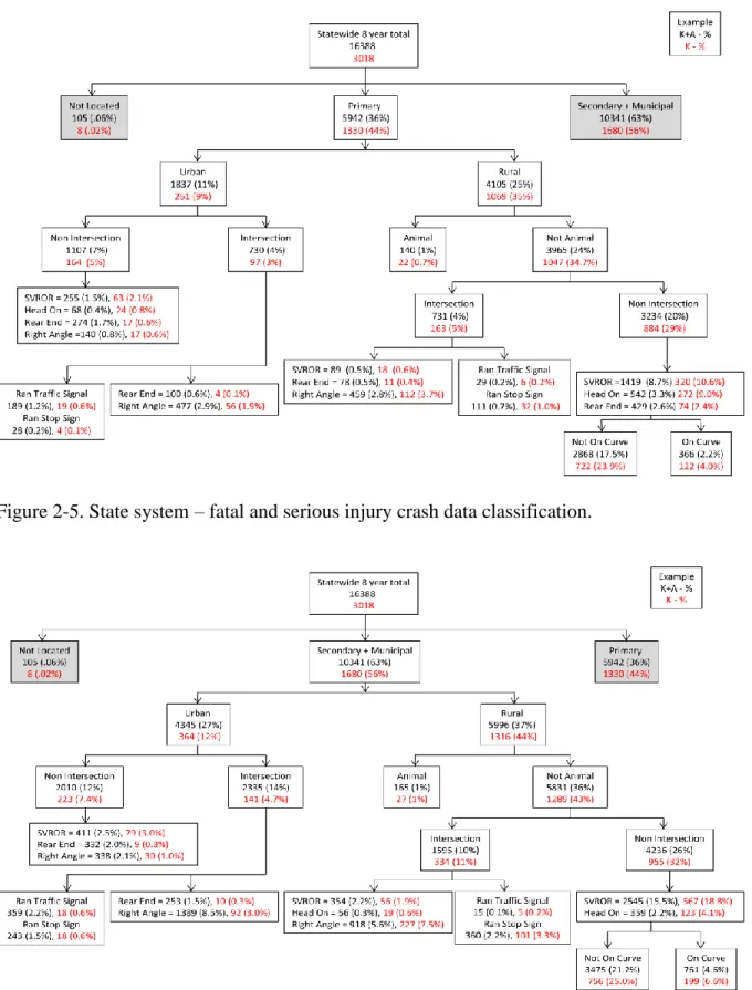
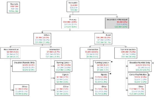
Crash data were classified first by system type (state and local) and then by urban and rural distinction. The local system in this analysis includes both secondary and municipal roadways. Figure 2-5 shows the classification of the primary system fatal and serious injury crashes. Figure 2-6 shows the classification of fatal and serious injury crashes on the local roadway system.
Figure 2-5. State system – fatal and serious injury crash data classification.
Of the 16,388 fatal and major injury crashes statewide during the 8 year analysis period, nearly two-thirds occurred on local roadways. For both the primary and local system there were about twice as many rural crashes as urban crashes. Furthermore there is a greater portion of fatal crashes on rural roadways than on urban roadways. Forty-four percent of all fatalities occur on the rural local system while 35 percent occur on rural primary roadways. Therefore over three in every four fatalities occurs on a rural roadway.
This over dispersion on the rural system can be attributed to a few factors. First, rural roadways tend to operate at higher speeds therefore the risk for a fatal crash is increased. Second, emergency response times for rural roadways are much higher than on urban roadways. According to a 1999 study for the International Symposium on Transportation Recorders the average elapsed time from the moment of the crash until the victim arrives at the hospital for rural fatal crashes is 17 minutes more than for urban fatal crashes (Champion. et. al, 1999). This additional time for emergency response on rural roadways could
contribute to a greater number of fatalities.
At intersections, right angle crashes account for the majority of fatal and serious injury crashes. Right angle crashes by nature tend to be more severe. Nearly 9 percent of the statewide fatal and serious injury crashes are right angle crashes occurring at urban
intersections on the local system.
Single vehicle run-off-road crashes are the most common non-intersection crash. Single vehicle run-off-road crashes tend to be primarily a rural roadway issue. Over 15 percent of all statewide K+A crashes and nearly 20 percent of all fatal crashes are local system run-off crashes. On the primary system, single vehicle run-off-road crashes account for 9 percent of the statewide K+A crashes and 11 percent of all fatal crashes.
2.5.2 Statewide allocation of safety funds
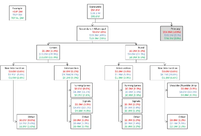
The second classification categorized safety project funds based on roadway on which the improvement was completed as well as by improvement type. Safety project data were first classified by system type (state and local) and then by urban and rural distinction. The local system in this analysis includes both secondary and municipal roadways. Projects
funded with HSIP funds and projects funded with TSIP funds were assessed separately and in total. Figure 2-7 illustrates the allocation of safety funding by project type and location on the state system. Figure 2-8 presents the same information for the local system.
Figure 2-8. Local system – allocation of funding by project type and location.
Of the $93 million invested in both the HSIP and TSIP projects, 80 percent of the total funding was allocated to the state system. All $55 million of the HSIP program funds from FY 2001-2009 were invested on the state system. Funding from the TSIP program allocated from FY 2004-20011 was balanced, more or less evenly, between the state and local system.
Approximately 65 percent of the combined HSIP and TSIP funding was invested on the rural state system. Furthermore, approximately a third of all combined HSIP and TSIP funding was allocated to shoulder and edge-line rumble strip projects. The ease of
implementation and relatively small capital cost of edge-line rumble strips make these types of projects very attractive. According to the Iowa DOT, “low-cost safety improvements (such as edge-line rumble strips, cable median barrier, and bigger and brighter curve and chevron signs) have proven to be very effective when data is systematically used to identify and address locations with high crash rates” (p.16, Iowa CHSP, 2006).
Adding turning lanes can reduce rear-end crashes but are not a right-angle preventative mitigation (CMF Clearinghouse, 2010). Urban intersections on the state system are allocated about 19 percent of all statewide safety funds. Urban intersections are often considered black spots because of high volumes of traffic and a large number of conflict points. “Common black spot locations are intersections, particularly signalized intersections along multi-lane urban arterial roadways” (p. 3 Preston et. al., 2010).
2.5.3 Combined crash data and safety project classification
After the crash data classification and safety project data classification were
completed, corresponding categories were matched. For example, crashes classified as road departures occurring at non-intersection locations on rural freeways were matched with the safety funding allocated to non-intersection, rural freeway improvements mitigating road departures (e.g. rumble strips, shoulder improvements). Once all categories of crash location and types were matched with their corresponding funding, the “relative difference” for each category was calculated. Figure 2-9 provides an example of how the “relative difference” was calculated using Equation 2-1.
different numbers of crashes and different amounts of funding to be compared relative to each other. To better depict how each category compares to one another, a “coloring scale” was created. Figure 2-10 shows the “color scale” used to visually compare different crash location and crash type categories.
Figure 2-10. “Relative difference” color scale.
The maximum difference between and was found to be 30.9. Thirty point nine is therefore used as in all “relative difference” calculations. The complete classification, matching crash data and safety funding, is shown in Figure 2-11, Figure 2-12, and Figure 2-13.
21
22
23
and signals mitigate more than one type of crash; some projects included multiple project types, while some descriptions did not include enough adequate details to connect them with a specific crash type. For these reasons, some projects and crash types were combined and excluded from the “relative difference” analysis. These categories are identified with a gray color box.
In Iowa it appears that rural and urban funding is nearly balanced with the amount of statewide crashes occurring in each respective area. However, a quick examination of the classification shows an apparent disconnect of funding between the state and local system. About 25 percent of the statewide fatal and serious injury crashes occurred on the rural state system yet 56 percent of the statewide funding was allocated to these roadways. In contrast, approximately 36 percent of the statewide fatal and serious injury crashes occurred on the rural local system and only 9 percent of statewide funding was allocated to these roadways. There are many reasons for this apparent disconnect as discussed in the following section.
Furthermore, rural state expressways, where only about 5 percent of statewide crashes occur, were allocated more than one fourth of all statewide expenditures. Most of the
projects on rural state expressways were shoulder and/or edge line rumble strip projects. On the rural local system, unpaved roadways received no funding, while paved roadways
received about 9 percent of the statewide funding as compared to the 23 percent of K+A crashes that occur on these roadways.
The urban state system received almost a fourth of the statewide funding, yet only 11 percent of the statewide fatal and serious injury crashes during the study period occurred on these roadways. Multi-lane divided intersections on the state system received more funding relative to the number of crashes that occurred on these roadways. The urban local system, which had about one fourth of all statewide K+A crashes, received only 12 percent of all statewide funds.
2.5.4 Safety funding allocation relative to crash density
Upon first inspection there appears to be a significant disconnect between the statewide crash incidence and the safety funding allocation. According to current state policy, funding through the HSIP program is only available for state system projects; local jurisdictions do not have access to that funding. Moreover, this funding accounts for 60 percent of the statewide funding ($54.9 million).
Like many states, Iowa invests safety dollars on more densely traveled roadways. Roadways such as rural, state expressways and multi-lane, urban roadways have received more funding because their crash densities are greater than other systems. The roadway systems with higher crash densities tend to receive more funding relative to number of crashes occurring on those systems. Figure 2-14 illustrates this investment in higher density roadways. Figure 2-14 shows the safety investment on Iowa roadways relative to the number of crashes on each system, with the average number of crashes per mile, per year from 2001-2008.
Figure 2-14. Relative safety investment for Iowa roadway classifications (crash densities show in parentheses).
it ever be more practical to invest safety dollars on roadway systems with many crashes spread over many miles of roadway like the classification analysis suggests? Consider this hypothetical example:
US Highway 218 directly south of Interstate 80 in Johnson County is a four-lane divided expressway. This 15.5 mile section of roadway has previously received funding from the HSIP program for paved shoulders and rumble strips. Assume that there is still a crash problem and the recommended mitigation is to flatten the sideslopes of the roadway from 1:4 to 1:6. Also consider a proposal to add milled-in rumble strips on 8 corridors, totaling 84.5 miles all on secondary, two-lane paved roadways. All of these corridors are from the 2009 Iowa 5 percent report and labeled as corridors with the highest fatal and serious injury crash density for single vehicle run-of-road crashes. The expressway project has a crash density of 4.7 crashes/mile/year compared to an aggregate crash density for all eight secondary roadways of 1.0 crashes/mile/year. Therefore if considering crash density, it would be recommended that the expressway project be completed over the secondary
roadway projects.
The following assumptions were made for the sideslope flattening project:
Assume other mitigations have been done and flattening the sideslope is the preferred option
Assume a constant and typical slope throughout the 15.5 mile segment
Assume the unit cost of fill/flattening is $3.08 CY (Iowa DOT Bid Express)
Assume flattening applies to roadsides and median
Assume each slope is 24’, therefore on average, need 3.00 yd2
to flatten slope from 1:4 to 1:6
Assume total CY of fill/flattening need is 327,360 CY
Assume estimated cost of crash by severity as per National Safety Council, 2009
The following assumptions were made for the rumble strip projects:
Assume roadways meet the minimum requirements for edge-line rumble strip projects in Iowa
Assume the unit cost of milled-in rumble strips is $658/mi/shoulder (Iowa DOT Bid Express)
Assume a constant and typical slope throughout the 15.5 mile segment Table 2-1 shows a comparison of these two proposed projects. The rumble strip projects on the rural, secondary, two-lane corridors yields a benefit/cost ratio (42.4) much higher than that of the rural expressway sideslope project (2.6). This is a good example of a project on a roadway with a lower crash density that should be implemented in lieu of a project on a high crash density roadway. Investing safety funds where it can make a difference is most prudent.
Table 2-1. Comparison of rural expressway sideslope flattening project and rural secondary two-lane rumble strip projects.
K A B C 0 Total K A B C 0 Total Rural State Expressway - Slope Flattening Project 15.5 0.5 2.125 8 8 54.13 72.75 0.76 0.38 1.62 6.08 6.08 41.1 55.29 $2,578,984 $1,008,269 2.6 Rural Secondary Two Lane -Rumble Strip Projects 84.5 1.13* 4.25* 6.00* 9.63* 12.75* 33.75* 0.74 0.83 3.15 4.44 7.12 9.44 24.975 $4,717,084 $111,202 42.4
Project Type Mileage Average Crashes Per Year (2001-2008)
cSource: http:www.bidx.com
bSource: National Safety Council (estimated cost of crash) aSource: CMF Clearinghouse
*SVROR crashes only
CMFa Average Crashes Mitigated Per Year Estimated
Benefitb
Estimated Costc
Estimated B/C
2.5.5 Black spot analysis vs. mass action analysis
Another consideration needed in the funding allocation process is the method utilized to identify and prioritize sites, corridors, or even systems for potential safety investment. The data identify the most common fatal and serious injury, intersection crash type as right angle. The most common fatal and serious injury, non-intersection crash type is single
and serious injury crashes from 2001 to 2008, while SVROR crashes account for 33 percent all fatal and serious injury crashes over the same period.
Historically, as identified by the literature, black spot analysis is the “most common method to identify candidate locations for safety investment” (p. 3, Preston et al., 2010). The Iowa 5 Percent Report and SICL List are two examples of the use of black spot analysis to identify and prioritize intersections and corridors for safety investment. These two processes are important and integral in addressing highway safety in Iowa but upon further inspection they only address a fraction of statewide crashes.
Table 2-2 compares the intersection crashes at the top 200 intersections, as prioritized by the SICL list for 2003-2007, to all statewide and intersection crashes for the same period. In Iowa there are approximately 160,000 intersections, therefore 17 percent of all fatal and serious injury crashes occur at the top 0.125 percent of all intersections. This is a very substantial number but it also means that 83 percent of all intersection crashes are spread across the other 150,800 intersections.
Table 2-2. SICL list crash comparison.
2.8% of all crashes
8.3% of all intersection crashes 4.8% of all K+A crashes
17.0% of all K+A intersection crashes Top 200 Intersection Crashes (2003-2007)
484 8264
Number of K+A crashes occuring at the top 200 intersections Number of crashes occuring at the top 200 intersections
Table 2-3 compares the SVROR fatal and serious crashes occurring on the top 33 corridors, as prioritized by the 2010 Iowa 5 percent report, to all SVROR fatal and serious injury crashes occurring between 2001 and 2008. The total mileage of these corridors is approximately 345 miles. The state of Iowa has approximately 115,000 miles of roadway statewide, with about 105,300 miles of which is rural. Therefore, approximately 4.1 percent of all SVROR crashes occur on only 0.3 percent of the total roadway network. This also means that over 4,527 fatal and major injury SVROR crashes are distributed over about 105,000 miles of rural roadways.
Table 2-3. Iowa 5 percent crash comparison for SVROR crashes.
1.2% of all K+A crashes 4.1% of all K+A SVROR crashes Top 33 SVROR Corridors by K+A Crash Density
Number of K+A crashes occuring at highest 33 SVROR crash
density corridors 195
Using a high crash location approach to mitigate these widely distributed crashes is not effective because it will not yield many locations that exhibit unusually high crash frequencies or crash rates. The only way to address these widely distributed crashes is to use a systematic approach. This does not suggest, however, that black spot analysis not be utilized; rather it suggests that there needs to be a balance between the two methods.
2.6 CONCLUSIONS AND RECOMMENDATIONS
Several questions were addressed through the classification of statewide crash data. It appears that not all of Iowa’s roadway system elements are equally at risk. For example, some facility types, such as state and local two-lane rural roadways are more at risk for single vehicle run-off-road crashes. The results of the matching of crash data with safety project funding data suggest the shifting of funds from the high crash density state system to facilities on the low density local system. However, it is clear that the redistribution of funds, from one system to another, includes many other factors such as crash density, benefit-cost, and other political issues.
The allocation of funding should also identify what mitigations have been
implemented and what additional options are available to maximize safety spending. It is very possible for a safety project on a roadway with a lower crash density to be more effective than a project on a roadway with a very high crash density, depending on the projects and their benefit/cost ratios. Crash reduction factors and benefit cost analyses are integral in aiding the safety funding decision making process as well. Ultimately, the optimum allocation of resources would reduce the most possible fatal and serious injury crashes.
Some crashes are too widely distributed over many miles of roadway to be identified as possible sites in need of safety mitigation. It was recommended that the highway safety
approaches. There should be a balance among these two methods. This optimum balance between black spot and mass action is yet to be determined. It is recommended that this balance of black spot and mass action be addressed in future research.
CHAPTER 3. SYSTEMWIDE IDENTIFICATION OF HORIZONTAL CURVES AND GEOMETERY PARAMETERS
3.1 INTRODUCTION
In order to analyze the safety performance of horizontal curves and mitigate associated crash problems, curve locations and characteristics must be known. However, curve identification is difficult on a large system. In Iowa, rural horizontal curves comprise of only 1.2 percent of the state’s total of 115,335 miles. Yet 10.5 percent of the state’s fatal crashes occur on these roadways.
Table 3-1 shows this over representation of fatal crashes on horizontal curves in Iowa. Nationwide more than 25 percent of fatal crashes are associated with horizontal curves
(FHWA). Crash rates for horizontal curves are typically 1.5 to 4 times higher than the crash rates of tangent highway sections (Zegeer, et al., 1992). Figure 3-1 shows the distribution of horizontal curves on paved, two-lane, rural highways in Iowa.
Table 3-1. Iowa statewide crash comparison for horizontal curves (2001-2009).
Fatal 353 2437 3355 14.5% 10.5% Injury 5384 50584 153362 10.6% 3.5% PDO 5861 108443 370195 5.4% 1.6% All 11598 161464 526912 7.2% 2.2% Statewide Crashes Curve Crashes/ Rural Crashes Curve Crashes/ Statewide Crashes Crashes on Curves Rural Crashes
Figure 3-1. Two-lane horizontal curve distribution with paved two-lane, rural roads shown in gray.
Recently the Iowa DOT has addressed safety concerns on horizontal curves. In 2010, the Iowa 5 percent report identified and prioritized horizontal curves based on crash
frequency. However past studies show that prioritization of horizontal curves needs to be based on more than just crash frequency (Preston et al., 2009). Other factors such as curve radii, traffic volume, the presence of visual traps, intersections and proximity to other high priority curves should also be considered (Preston et al., 2009).
The purpose of this chapter was to first create a statewide curve database by systematically identifying horizontal curves on two-lane rural roads in Iowa. Secondly, a validation of the curve identification methods was completed using a sample of curves with as-built geometric data. Lastly, the safety performance of horizontal curves in Iowa was explored using crash prediction models. Chapter 4 of this thesis presents the crash prediction model based on these data.
3.2 REVIEW OF LITERATURE
The most widely used method of curve geometry data collection includes the use of an in vehicle GPS receiver and some form of post-processing. Patterson, D., et al. (2006) used GPS and GIS applications to collect and analyze horizontal curve geometry data. The process included collecting field data at 0.1-second intervals using differential GPS
surveying in a vehicle. Results demonstrated that GPS could quickly, accurately, and inexpensively produce horizontal alignment data.
Pratt, et al. (2009) used a similar method to collect curve geometry while driving through a curve. A GPS receiver was used to collect curve radius and deflection angle data. An electronic ball-bank indicator was used to gather superelevation data. These two
instruments were directly connected with a laptop, and, while driving, curve data were simultaneously compiled into an in house software package called the Texas Roadway Analysis and Measurement Software (TRAMS). Data were collected at 25 foot increments, and curve radii were calculated. These data were then post-processed to calculate a
recommended advisory speed. Results showed that this method provided an accurate and precise measurement of curve radius. However, these methods are impractical for collection of statewide curve data.
Sanders (2007) provided a methodology for statewide data collection of horizontal curves using GPS centerlines. GPS data for over 79,000 centerline miles of roadway were collected in Kentucky. An automated process was developed using GIS to extract curve data and determine roadway geometry. Results showed this GPS/GIS method provided much more accurate curve data than previous field-collected processes.
3.3 DATA
3.3.1 Roadway data
In this study, Iowa statewide road data were obtained from the 2007 GIMS roadway database. The complete GIMS database was reduced because the focus of this study is rural two-lane facilities. Rural, two-lane facilities with a speed limit of 45 mph or greater were extracted from the complete roadway dataset.
Calculated curve data were obtained through a manual identification process
discussed in the methodology section of this chapter. The GIMS 2007 database was used for roadway attributes. The Iowa Pavement Management Program (IPMP) provided GPS traces of the state’s roadways, originally obtained from in-vehicle GPS data collectors. The data consist of points at ten meter increments along all paved routes throughout the state.
3.3.3 As-built curve data
As-built data were required for the validation of the calculated curve data geometry. As-built curve data were identified using the Iowa DOT’s Electronic Records Management System (ERMS). ERMS contains historic roadway plans for all primary road projects in Iowa. Secondary (county) road data were not available in the ERMS and were not included in the study.
Curve data available in the historic roadway plans were manually extracted for a specific set of counties. Data for 435 horizontal curves were identified in 15 counties throughout Iowa. Figure 3-2 shows the counties in which horizontal curve data were identified. Horizontal curve data were collected on paved two-lane rural roadways with a speed limit of 45 mph or greater to match the roadways used to identify curves in the created horizontal curve database. Curve data were extracted by county because roadway plans in ERMS are stored by county. Counties were chosen to yield a sample that is topographically diverse and geographically dispersed throughout the state.
Figure 3-2. Plan set curve data locations.
3.4 METHODOLOGY
3.4.1 Curve identification
Horizontal curves were identified with the use of GIS tools. To limit the extent of required visual inspection and to more systematically identify possible locations of horizontal curvature, polylines were first created, and later simplified, from the available IPMP GPS traces. The remaining vertices in the simplified polylines primarily represented the locations of route termini and, more importantly, possible curvature. GPS traces from IPMP, the GIMS roadway network and the simplified polyline vertices were then added into an ArcGIS workspace for visual inspection. Aerial imagery was also used as a reference, where
necessary.
Once a reviewer identified a section of roadway as a horizontal curve, the GPS traces were selected and manually coded as being a part of a curve. Post-processing was then performed on the GPS traces to extract only the “curve” records, combine the points for each
identified, they were compiled and reintroduced to the GIS environment for analysis. Figure 3-3 shows a roadway (black line), the location of the GPS traces (small green dots) and the location of the simplified polyline vertices (large green dots). The red line shows the final approximate location of the curve relative to the tangents.
Figure 3-3. Curve identification process with GPS traces and simplified polyline vertices.
Spiral transition data were not collected. The reviewer identified possible locations of roadway curvature only. Every curve was assumed to be a circular curve in order for the radius value to be estimated using circular regression during post-processing. Therefore, if a curve was located it was assumed to be a circular curve.
Estimated curve geometry included length, degree of curvature, and two different radius values. The first curve radius value was calculated using circular regression. Once a curve was identified, a circle was fitted through each GPS trace of the curve to find a best fit. The radius of that circle was the estimated radius of the curve. This radius value is referred to as Rregression. In order for a curve to be fit, a curve was required to have at least five GPS
traces associated with it. If a curve did not have five traces associated with it, the post-processing would not work properly and the Rregression value would be estimated as zero.
The second radius value was calculated using the long chord of the curve. A straight line was fitted through the reviewer’s estimated point of curvature (PC) and point of
tangency (PT) for each curve. The radius value was then estimated using the long chord and the angle between the long chord and curve. This radius value is referred to as Rchord. For
simplicity and mass production the processes used to estimate both radius values where performed using a macro program in Microsoft Excel.
3.4.2 Curve identification validation process
In order to validate the curve identification process, as-built horizontal curve data needed to be compared to the estimated curve data for a sample of curves. As previously mentioned, as-built curve data were extracted from historic roadway plans using ERMS and compiled. A unique, as-built identifier, different from the unique identifier for the curve identification process, was given to each curve. The location of the horizontal curves was then found using Google Map tools. The unique, as-built identifier was then matched and attached to its corresponding horizontal curve data using GIS tools. Once this process was completed, as-built curve data could be compared with the estimated curve data and validated for precision.
Percent RMSE was used as a measure of precision to validate the curve identification process. RMSE measures the deviation between the actual geometric feature value (e.g. length, radius), and the estimated geometric feature value. A large percent RMSE indicates a large deviation between the actual and estimated values.
Equation 3-1:
√∑ (∑ )
= calculated geometric feature value (e.g. Lpredicted, Rreg, Rchord)
= as-built geometric feature value (e.g. Lactual, Ladjusted, Ractual)
= number of horizontal curves
Further analysis was completed to investigate the relationship between percent error and geometric features as well as how well the sample represents the entire database. In order to explore the representation of roadway curves, the coincidence ratio was compared between the histogram of the sample of curves with as-built data and the histogram of all
secondary curves). Histograms were compared for curve length and both radius estimation methods. The estimated curve length values were divided into “bins” at 100 foot increments while both estimated radius values were divided in increments of 250 feet.
The coincidence ratio compares two distributions and measures the percentage of total area in common between the two distributions. It should be noted that the coincidence variable is only used to check whether or not the sample is representative of the entire
population and is not a measure of precision. Equation 3-2 shows the formula for calculating the coincidence ratio.
Equation 3-2:
∑ {
} ∑ { }
= frequency of geometric values (e.g. Rregression) with radius value j from sample of
curves
= frequency of geometric values (e.g. Rregression) with radius value j from population of
curves (or primary roadway curves)
= total number of geometric values (e.g. Rregression) in sample of curves (329)
= total number of geometric values (e.g. Rregression) in population of curves (11,279) or
primary roadway curves (2,349)
3.5 ANALYSIS
11,882 curves were identified during the curve identification process. If a curve did not have at least five GPS traces assigned to it the Rregression value would be estimated as zero.
Of the 11,882, 603 had less than five GPS traces and therefore an Rregression value of zero.
Because of the zero value for the Rregression, these curves were removed from the analysis.
Therefore a total of 11,279 curves were included in the statewide horizontal curve database. Table 3-2 gives the number of horizontal curves identified and the average curve geometry for the primary and secondary systems. As expected, curves on secondary
roadway curves, tend to be shorter in length and have a sharper radius.
Table 3-2. Identified curves by system type.
L (ft) Rregression (ft) Rchord (ft)
Primary 2349 870 2162 2078
Secondary 8930 576 1158 1136
All 11279 637 1367 1332
Average Curve Geometry Number of
Curves Roadway
System
Using the historic roadway plans, as-built data were identified for 435 curves on the primary system. Of these, 329 were matched with curves from the statewide curve database. The curves that were not matched were mostly large radius curves that were so large they were not identified as curves in the manual identification process. A few curves were matched, but upon further inspection were found to have incorrect data. These curves were omitted.
3.5.1 Horizontal curve length estimation
Figure 3-4 shows the actual horizontal curve length plotted against the estimated horizontal curve length. The curve length was estimated during the curve identification process by manually estimating the PC and PT locations. The percent RMSE of the curve length is 29.03 percent. This magnitude error was expected for the curve length because of the way curve lengths were estimated. It is difficult to identify exact location of where the curve ends and begins. Furthermore there appears to be a systematic bias to underestimate the curve length. These sources of error are discussed further in the “Sources of error” section of this chapter.
Figure 3-4. Actual curve length vs. estimated curve length.
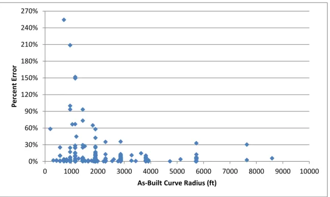
The absolute, percent error between the estimated curve length and as-built curve length versus the as-built curve length is plotted in Figure 3-5. One would expect as the curve length increases, the percent error would decrease. However, the percent errors do not necessarily follow this form although all large errors (>60 percent) are on curves shorter than 1,500 feet in length. Eighty-seven percent of all estimated curve length data have a percent error of less than 40 percent.
0 500 1000 1500 2000 2500 3000 3500 0 500 1000 1500 2000 2500 3000 3500 Esti m ate d Len gth (ft) Actual Length (ft)
L
actualvs L
estimated %RSME= 29.03%Figure 3-5. Curve length versus percent error of estimated length value.
Figure 3-6 shows both the curve length histogram for the sample of curves with as-built data and the curve length histogram for all curves identified on primary roadways. Comparing the two histograms yields a coincidence ratio of 0.826, indicating that 82 percent of the primary roadway data length values are described by the sample of curves with as-built data.
When comparing the curve length histogram for the sample of curves to the curve length histogram of the entire population of curves (primary and secondary roadways) the coincidence ratio decreases to 0.580. Figure 3-7 displays both the curve length histogram for the sample of curves data and the curve length histogram for the entire population of
identified curves.
The reason for this decrease is due to the inclusion of secondary roadway curves. Since the sample of curves data contain only data from primary roadway curves, the sample of curves is a better representative of the primary roadway curve data. Secondary roadways, on average have shorter length curves and therefore the population of curves histogram is skewed towards shorter length curves.
0% 20% 40% 60% 80% 100% 120% 140% 0 500 1000 1500 2000 2500 3000 3500 Per ce n t Er ro r
Figure 3-6. Curve length histogram comparison for sample curves and primary roadway curves.
Figure 3-7. Curve length histogram comparison for sample curves and all curves in database.
3.5.2 Horizontal curve radius estimation using the circular regression method
Figure 3-8 shows the actual, as-built curve radius plotted against the calculated curve radius using the circular regression method, Rregression. The circular regression method is
0 0.02 0.04 0.06 0.08 0.1 0.12 Fr e q u e n cy
Estimated Curve Length (ft)
Primary Road Curves (2349) Sample Curves (329)
Coincidence Ratio 0.826 0 0.02 0.04 0.06 0.08 0.1 0.12 0.14 0.16 0.18 Fr e q u e n cy
Estimated Curve Length (ft)
Curve Population (11,279) Sample Curves (329)
Coincidence Ratio 0.580