Generalized Linear Longitudinal Semi-parametric
Models with Time Dependent Covariates
St. John's
by
© V
ineetha Warriyar K. VA thesis submitted to the School of Graduate Studies
in partial fulfilment of the requirements for the degree of
Doctor of Philosophy
Department of Mathematics and Statistics Memorial University of Newfoundland
November 2012
Abstract
Longitudinal data analysis is challenging because of the difficulties in modelling the correlations among the repeated responses, especially when the associated covariates are time dependent. Recent studies have examined correlations for both linear and discrete unbalanced longitudinal data, which are modelled following a Gaussian-type auto-regressive moving average (ARMA) class of auto-correlations. However, these studies were confined to a regression setup where the regression function is completely specified. In this thesis, we consider a semi-parametric regression setup in which the regression function involves a specified as well as an unspecified function over time. Under the ARMA type correlation structure, we provide a semi-parametric gener-alized quasi-likelihood (SGQL) approach for the estimation of the main regression parameters. The proposed inference approach is compared with some existing gener-alized estimating equation (GEE) approaches mainly through simulation studies. The linear longitudinal semi-parametric model, for its foundational nature, is discussed in detail. Theoretical details on semi-parametric estimation for longitudinal count and binary data are also provided.
Acknowledgements
I would like to express sincere thanks to my supervisor, Dr. Brajendra Sut rad-har. His support, vast knowledge and logical way of thinking have been invaluable throughout my work.
Thanks to all my friends, colleagues and house mates for putting up with me. I owe a great deal for their encouragement and moral support.
A special thanks to the Department of Mathematics and Statistics at Memorial University for providing financial and academic assistance for my research, especially all administrative staff members for the help they offered me during my study.
I would like to thank all the examiners of my thesis Dr. Mary Thompson, Dr. Gary Sneddon and Dr. Alwell Oyet for their invaluable comments and suggestions.
I am so indebted to my parents, my sister, my in-laws, and my uncle Dr. Asokan. M. Variyath, who motivated me to explore the wonderful world of Statistics, for their constant support and encouragement. Indeed, I am grateful to my husband, Ranjith, for his encouragement, coufidence and forbearauce. Without my family's understanding and love, I would not have been able to finish this thesis. Above all, I thank Almighty God, without whose blessing I would never have been able to complete this work.
I lovingly dedicate this thesis
Contents
Abstract
Acknowledgements
List of Tables
List of Figures
1 Background of the Problem
1.1 Generalized linear models ( G LMs) . 1.1.1 Quasi-likelihood estimation for (3 1.2 Semi-parametric GLMs .
1.2.1 Linear model . .
1.2.1.1 Estimation of non-parametric function 1(z0)
1.2.1.2 Estimation of regression effects (3 1.2.2 Count data model . . .
1.2.2.1 Estimation of non-parametric function 1(z0) 1.2.2.2 Estimation of regression effects (3
1.2.3 Binary data model . . . . . . . . .
11 111 Vl V11 1 2 3 4 6 7 8 9 10 11 12
1.2.3.1 Estimation of non-parametric function 'Y(z0 ) 1.2.3.2 Estimation of regression effects /3
1.3 Generalized linear longitudinal models (GLLMs) 1.4 Semi-parametric GLLMs
1.5 Objective of the thesis .
2 Semi-parametric Linear Longitudinal Models 2.1 Existing semi-parametric estimation methods
2.1.1 PSSGEE approach .. . . .. . 13 13 14 17 18 21 28 28
2.1.1.1 Estimation of non-parametric function 29
2.1.1.2 Estimation of regression effects . . . . 31 2.1.1.3 Estimation of the 'working' correlation parameter a . 32 2.1.2 Partially standardized emi-parametric heteroscedastic GEE (PSSHGEE)
approach. 33
2.2 Proposed FSSGQL approach . 35
2.2.1 Estimation of non-parametric function 35
2.2.2 Estimation of (3 36
2.2.2.1 Basic properties of !3FsscQL 38
2.2.3 Estimation of p and a2 43
2.3 A Simulation study 45
2.3.1 Simulation design 45
2.3.2 Data generation and simulation results 47
3 Semi-parametric Longitudinal Models for Discrete Data with
3.1 Semi-parametric longitudinal models for count data with non-stationary correlation structures . . . . . . . . . . . 72 3.1.1 Stationary correlation models for count data in emi-parametric
etup . . . . . . . . . . . . . . . . 73 3.1.2 on-stationary correlation models for count data 74 3.1.2.1 Non-stationary AR(1) models in semi-parametric setup 74 3.1.2.2 on-stationary MA(1) models in semi-parametric setup 76 3.1.2.3 Non-stationary EQC models in semi-parametric setup 77 3.2 Estimation in semi-parametric models for longitudinal count data 7
3.2.1 E timation of non-parametric function 1(.) 78 3.2.2 Estimation of
f3
. .
.
.
.
.
.
. . .
.
.
.
. .
793.2.2.1 Naive GQL estimation approach 79
3.2.2.2 PSSGQL estimation under non-stationary (ns) corre-lation structure . . . . . . . . . . . . . . . .
3.2.2.3 Estimation of correlation index parameter p
3.2.2.4 FSSGQL estimation under non-stationary correlation
3.2.2.5 3.2.2.6
structure
Existing PSSGEE approach
Estimation of 'working' correlation parameter a
3.3 Semi-parametric longitudinal models for binary data with non-stationary correlation structures . . . . . . . . . . . . . . . . 80 82 84 88 89
90
3.3.1 Non-stationary correlation models for binary data 91 3.3.1.1 Non-stationary AR(1) models in semi-parametric setup 91 3.3.2 on-stationary MA(1) models in semi-parametric setup . 923.3.3 Non-stationary EQC models in semi-parametric setup . . . 93 3.4 Estimation in semi-parametric models in longitudinal binary data 94
3.4.1 Estimation of non-parametric function 1 (.) 3.4.1.1
3.4.1.2 3.4.1.3
PSSGQL(ns) estimation of
f3
Estimation of correlation index parameter p . FSSGQL(ns) estimation of f3
...
.
.... .
94 96 98 98
4 Empirical Study for Semi-parametric Longitudinal Count Data M od-els
4.1 Simulation design 4.2 Data generation
4.3 NGQL estimation: A biased approach
4.4 A finite sample efficiency comparison between PSSGQL(ns) and PSS-G EE estimations . . . . . . . . . . . . .
4.5 Performance of the FSSGQL(ns) estimation
5 Concluding Remarks Bibliography 100 101 102 103 106 118 122 124
List of Tables
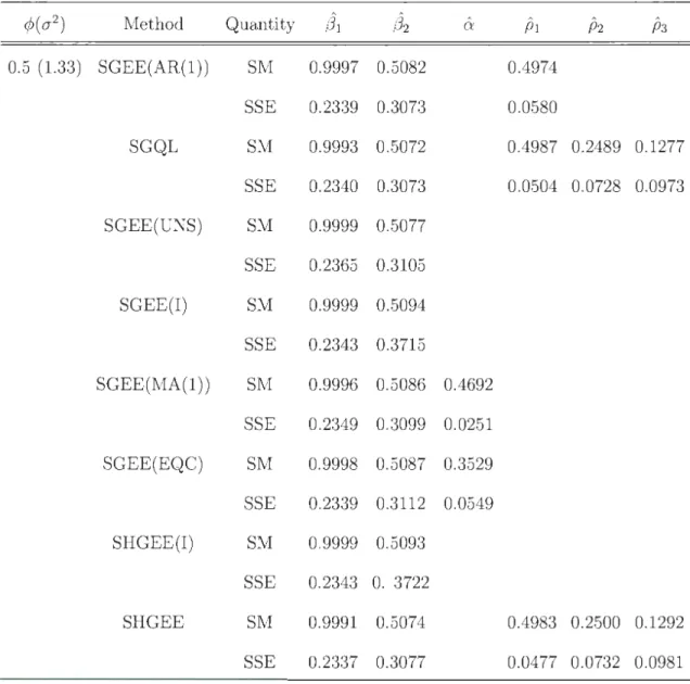
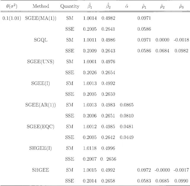
2.1 Simulated means (SMs) and simulated standard errors (SSEs) of the
estimates of regression parameters (31 = 1 and (32 = 0.5, under AR(1)
correlation model for selected values of the model parameters ¢ and 0'2; with ry(t) = 3
+ 2(t-
n;
1)+
(t -n
;
1 )2; K=100; n=4; and 1000simulations. . . . . . . . . . . . . . . . . . . . . . . . . . 55
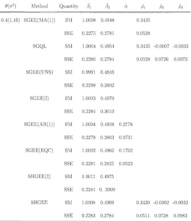
2.2 Simulated means (SMs) and simulated standard errors (SSEs) of the
estimates of regression parameters (31 = 1 and (32 = 0. 5, under MA ( 1) correlation model for selected values of the model parameters (} and 0'2; with ry(t) = 3
+ 2(t
-n;
1)+ (t-
n;
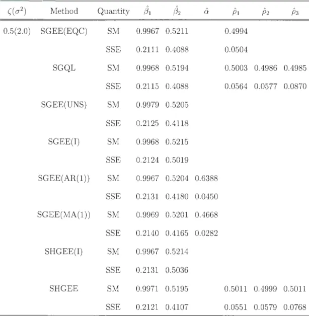
1 )2; K=100; n=4; and 1000 simulations. . . . . . . . . . . . . . . . .2.3 Simulated means (SMs) and simulated standard errors (SSEs) of the estimates of regression parameters (31 = 1 and (32 = 0.5, under equi correlation model for selected values of the model parameters ( and 0'2; with ry(t) = 3
+
2(t-n
;
1)+
(t-
n
;
1 )2; K=100; n=4; and 100057
2.4 Simulated means (SMs) and simulated standard errors (SSEs) of the
estimates of regression parameters (31 = 1 and (32 = 0.5, under AR(1) correlation model for selected values of the model parameters ¢ and
a2
; with 1(t) = sin2t; K=100; n=4; and 1000 simulations. . . . . . 61 2.5 Simulated means (SMs) and simulated standard errors (SSEs) of the
estimates of regression parameters (J1 = 1 and (J2 = 0.5, under MA(1) correlation model for selected values of the model parameters
e
and a2; with r (t) = sin2t; K=100; n=4; and 1000 simulations. . . . . . . . 63 2.6 Simulated means (SMs) and simulated standard errors (SSEs) of theestimates of regression parameters (31 = 1 and (32 = 0.5, under equi correlation model for selected values of the model parameters ( and
a2; with r (t) = sin2t; K=100; n=4; and 1000 simulations. . . . . . . . 65
4.1 Simulated means (SMs), simulated standard errors (SSEs) and mean squared error (MSEs) of the naive estimates of regression parameters (3 under non-stationary AR(1) correlation model for selected values of correlation index parameter p with K=100; n=4; and 1000 simulations. 104 4.2 Simulated means (SMs), simulated standard errors (SSEs) and mean
squared error (MSEs) of the PSSGQL and PSSG EE estimates of reg res-sion parameters {31 = 0.0 and (32 = 0.0, under non-stationary AR(1) correlation model for selected values of correlation index parameter p with K=100; n=4; and 1000 simulations. . . . . . . . . . . . . . 112
4.3 Simulated means (SMs), simulated standard errors (SSEs) and mean squared error (MSEs) of the PSSGQL and PSSGEE estimates ofregres
-sion parameters (31 = 1.0 and (32 = 1.0, under non-stationary AR(l) correlation model for selected values of correlation index parameter p with K=lOO; n=4; and 1000 simulations. . . . . . . . . . . . . . . . . 114 4.4 Simulated means (SMs), simulated standard errors (SSEs) and mean
squared error (MSEs) of the PSSGQL and PSSG EE estimates of regres -sion parameters (31 = 0.5 and (32 = 0.5, under non-stationary AR(l) correlation model for selected values of correlation index parameter p with K=lOO; n=4; and 1000 simulations. . . . . . . . . . 116 4.5 Simulated means (SMs), simulated standard errors (SSEs) and mean
squared error (MSEs) of the FSSGQL(ns) estimates of regression pa -rameter (3 under non-stationary AR( 1) correlation model for selected values of correlation index parameter p with K=lOO; n=4; and 1000 simulations. . . . . . . . . . . . . 119
List of Figures
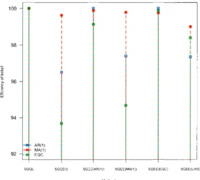
2.1 Efficiency comparisons of various semi parametric methods for the es-timates of (31 with '"Y(t) = 3 + 2(t - ntl) +
(
t -
ntl )2, under selected correlation processes: AR(l) with ¢ = 0.8, MA(l) withe
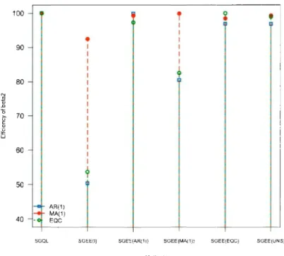
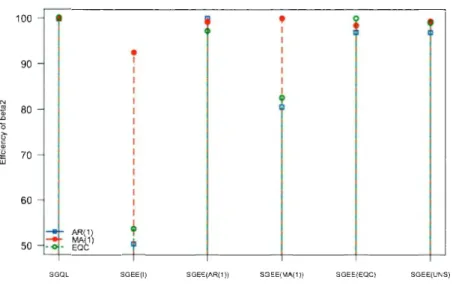
= 0.4 and EQC with ( = 0.8. . . . . . . . . . . . 0 0 0 0 0 • • • • • • 51 2.2 Efficiency comparisons of various semi parametric methods for thees-timates of (32 with '"Y(t) = 3 + 2(t - ntl) +
(t
-
ntl )2, under selected correlation processes: AR(l) with ¢ = 0.8, MA(l) with fJ = 0.4 and EQC with ( = 0.8. . . . . . . . . . . . . . . . . . 0 0 0 0 0 • • • • • • 52 2.3 Efficiency comparisons of various semi parametric methods for thees-timates of (31 with '"Y(t) = sin2t, under selected correlation processes: AR(l) with ¢= 0.8, MA(l) withe= 0.4 and EQC with ( = 0.8. . . . 53 2.4 Efficiency comparisons of various semi parametric methods for the
es-timates of (32 with '"Y(t) = sin2t, under selected correlation processes: AR(l) with¢ = 0.8, MA(l) withe = 0.4 and EQC with ( = 0.8. . . . 54
2.5 Simulated means of estimates of the non-parametric function ('y(t)
=
3+
2(t- 4!
1)+
(t- 4!
1 )2) under the true correlation matrix (TCM) and other selected correlation based FSSGQL method with AR(1) cor -related errors. . . . . . . . . . . . . . . . . . . . . 67 2.6 Simulated means of estimates of the non-parametric function ('y(t)=
3
+
2(t - 4!
1)
+
(t - 4!
1 )2) under the true correlation matrix (TCM) and other selected correlation based FSSGQL method with MA(1) co r-related errors. . . . . . . . . . . . . . . . . . . . . . . . . . 68 2.7 Simulated means of estimates of the non-parametric function ('y(t)=
3+ 2(t- 4
!
1) + (t- 4!
1 )2) under the true correlation matrix (TCM) and other selected correlation based FSSGQL method with Equi correlated errors. . . . . . . . . . . . . . . . . . . . . . . . . . . . . . . 69 2.8 Simulated means of estimates of the non-parametric function ('y(t) =sin2t) under selected correlation based FSSGQL method with Equi correlated errors. . . . . . . . . . . . . . . . . 70
4.1 Simulated means of estimates of 1(t) for PSSGQL and PSSGEE me th-ods, and true values of 1(t) under non-stationary AR(1) correlation models for count data with a correlation index parameter p
=
0.8 and regression parameters ({31 , {32 )'=
(0, 0)'. . . . . . . . . . . . . 109 4.2 Simulated means of estimates of 1(t) for PSSGQL and PSSGEE meth-ods, and true values of 1(t) under non-stationary AR(1) correlation models for count data with a correlation index parameter p
=
0.8 and4.3 Simulated means of estimates of 1(t) for PSSGQL and PSSGEE meth
-ods, and true values of 1(t) under non-stationary AR(1) correlation models for count data with a correlation index parameter p
=
0.8 andregression parameters ({31, {32)'
=
(0.5, 0.5)'. . . . . . . . . . . . 1114.4 Simulated means of estimates of 1(t) for FSSGQL(ns) method and true
values of '"'! ( t) under non-stationary AR( 1) correlation models for count
data with regression parameters ({31 , {32 )'
=
(0, 0)'. . . . . . . . 1204.5 Simulated means of estimates of 1(t) for FSSGQL(ns) method and true values of'"'!( t) under non-stationary AR( 1) correlation models for count
Chapter 1
Background of the Problem
Longitudinal studies are common in many scientific research areas such as clinical tri -als, economics, public health, agriculture, and so on. In these studies, the responses along with the covariates are collected from individuals over a period of time. In many cases, the time points are equally spaced. For example, (1) the Ohio asthma data [Zeger, Liang and Albert (1988)] collected from 537 children every year over a period of four years; (2) the health care utilization data [Sutradhar (2003, page 391)] collected by the General Hospital of the city of St. John's, Newfoundland, Canada, which contains the number of yearly visits to a physician by individuals over four consecutive years; and (3) the survey of labour and income dynamics (SLID) data on unemployment status among others collected by Statistics Canada [Sutradhar (2011)] every year over a period of six or more years. There are other situations where a re-spondent reports a response whenever an event occurs, where time points may not be equi-spaced. Because the repeated data are likely to be correlated, it is impor -tant to take such correlations into account for efficient inferences of the regression
effects involved in the model. However, the modelling of the correlations especially
when the responses are discrete is difficult even if the responses are collected over
equi-spaced time points. In a fixed regression setup, Sutradhar (2010) suggested a
Gaussian-type ARMA class of auto-correlation models appropriate for both linear
and discrete longitudinal data. These regression models however, may be inadequate in situations where a specified (or fixed) regression function may not be sufficient
to interpret the responses completely. In such cases, one may extend these models by adding an unspecified non-parametric function in time with the fixed regression
function. This leads to a semi-parametric regression model setup where longit u-dinal responses still follow a suitable correlation structure. There exists generalized estimating equation (GEE) based approaches to deal with the inferences for the afore -mentioned semi-parametric models in the longitudinal setup, where the modelling of longitudinal correlations are not done. In this thesis, however, we concentrate on the semi-parametric inferences for repeated data which follow a ARMA-type class of
auto-correlations. In order to give a background for this semi-parametric modelling and inference problem in the longitudinal setup, we first provide the notations and an overview for the semi-parametric problem in independence setup in Sections 1.1 and 1.2. A brief overview of the same semi-parametric problem in longitudinal setup
is provided in Sections 1.3 and 1.4.
1.1
Generalized linear models ( G LMs)
Consider a GLM regression set up [ Ielder and Wedderburn (1972)] in which an exponential family based independent responses {y-i}, i
=
1, ... , K are observed.Let Xi = (xi1 , ... , Xip)' be a multidimensional covariate vector corresponding to Yi for
the ith individual. Suppose that the mean response f.-Li(/3)
=
E(Y;) is influenced by aspecified fixed regression function (linear predictor) x~/3 with (3
=
(/3
1, ... , /3p)'· Thedensity of the exponential family based response Yi can be written as
(1.1)
where a(.) and b(.) are known functional forms such that b(.) depends only on Yi, and
the canonical parameter ei is defined with a suitable link function h(.) as
(1.2)
The parameter ei is related to the mean response through
(1.3)
where a'(.) is the first derivative of a(.) with respect to ei· Also, it follows that the
variance of Yi is
(1.4) where a"(.) is the second derivative of a(.) with respect to Bi·
1.1.1
Qu
as
i-lik
e
lihood
est
i
ma
ti
o
n f
or
{3
In the above exponential setup, the regression parameter (3 is involved in f.-Li ((3) = a' ( Bi)
as well as in aii ((3)
=
a" ( ei). Since aii ((3) is a function of the mean response, it is sufficient to estimate (3 involved in f.-Li(/3). When the density function is not known, and the mean and variance are given, Wedderburn (1974) proposed the quasi-likelihood(QL) estimation approach to estimate the regression parameter. In this approach,
one solves the QL estimating equation
t
aa~~i)
[a"(Bi)r1(Yi- a'(Bi)) =
t
81
~~)
[crii(,8)]-1(Yi- f-li(,8)) = 0 (1.5)i=l i=l
[see also McCullagh (1983), McCullagh and Neider (1989)]. The estimate ~QL
ob-tained by solving (1.5) is consistent and highly efficient. This is because under the exponential family setup, the QL estimate turns out to be the likelihood estimate,
which is known to be optimal (highly efficient). [Sutradhar (2010a)].
1.2
Semi-parametric GLMs
In semi-parametric models, the mean response f-Li(,8) depends not only on a fixed
regression function, but also on an unspecified (non-parametric) smooth function,
namely r(zi), where Zi is an auxiliary covariate which influences the response Yi· Then f-Li (,8) becomes a function of an unknown parameter vector
,8
and an unknown smooth function r(zi), which we abbreviate as(1.6)
In this set up, the canonical parameter
e
i
defined in (1.2) has the form(1.7)
It is clear that the main regression parameter
,8
can no longer be estimated unbiasedlyby ignoring the estimation of r(zi)· The semi-parametric GLMs are more flexible than the parametric GLMs especially when the regression function in fixed covariates is
Even though the estimation of both fixed regression parameter vector (3 and the non-parametric function 1(.) are of interest, many early works [ Staniswalis (1989), and Muller (1988)] concentrated on the estimation of the non-parametric mean func-tion, which is the same as substituting (3
= 0
in (1. 7). To deal with this type of non -parametric regression estimation there exists many kernel methods and its variants, such as the N adaraya-Watson kernel regression estimation [N adaraya ( 1964), W at-son (1964), Bierens (1987), Andrews (1995)], local linear and polynomial regression [Cleveland (1979), Fan (1992, 1993), Stone (1980, 1982)], recursive kernel estimation [see e.g., Ahmad and Lin (1976), Greblicki and Krzyzak (1980)], spline smoothing [Whittaker(1923), Eubank (1988), Wahba (1990)], and nearest neighbour estimation [Royall (1966), Stone(1977)]. Among these techniques, the simpler Nadaraya-Watson kernel estimator or the local constant estimator for 1 ( z) at a given covariate levelz = z0 involved in the linear model,
has the form
"\"'K , . K*(zo-z;) '(z ) = D i=lYt b I 0 "\"'K K*(zo-z;)
D t=l b
where K*(.) is a suitable kernel density function and b is known as the bandwidth. The selection of an appropriate bandwidth parameter b is always a problem in non-parametric regression [ Silverman(1986)]. In practice, we try to use a possible value of b for which the bias and variance of the estimator will be minimum. Many data -based methods such as cross validation [see Stone (1974), Picard and Cook (1984), Ansley, Kohn, and Tharm (1991)], generalized cross validation [Craven and Wahba
(1979)] were discussed in the literature for choosing an appropriate b. Altman (1990) suggested that these commonly used bandwidth selection techniques do not perform well when the errors are correlated. Hence we excluded these techniques and followed Pagan and Ullah (1999) who proposed an optimum value for bandwidth, which min -imizes the approximate mean integrated squared error. The authors recommended b ex n-115, and suggested that this value of bandwidth is the only value of b for which the bias and variance are of the same order of magnitude. Thus, as a practical choice, we will consider b = K-115.
In the independence set up, the estimation of both (3 and 1'(.) are also extensively
studied in the literature [e.g., Severini and Staniswalis (1994), Carota and Parmigiani (2002)]. Under the exponential family, for example, Severini and Staniswalis (1994) suggested a semi-parametric QL (SQL) approach for the estimation of (3 and f'(.).
The authors illustrated their estimation methodology using examples with linear, gamma and binary data. Note that we do not deal with (continuous) gamma data in the thesis, instead, we concentrate on modelling and inferences for linear and discrete data such as count and binary data in semi-parametric set up for independent and longitudinal responses. For convenience, we now provide semi-parametric QL estimation in details for linear, count and binary data in the independence set up.
1.2.1
Linear mod
e
l
Consider the model
where Ei's are independent and identically distributed with mean 0 and variance
O";
.
identity function. Also, var(Yi)
=
O"
ii
=O";
,
i = 1, ... , K.1.2.1.1 Estimation of non-parametric function 1(z0 )
For model (1.8), the quasi-likelihood function Q(f..li, Yi) can be written as
Then, the semi-parametric QL estimating equation for 1(z0 ) is
(1.9) ( ) Pi(ZQ~Zj) where wi zo = L~1Pi(¥l' Pi(.) being a kernel density function. For example, one may choose Pi( zo-;;z;) = vkb exp( -;1 ( zo-;;z; )2) with a suitable bandwidth b. Note that when wi(z0 ) = 1, this SQL equation further reduces to the well-known quas i-likelihood estimating equation [Wedderburn (1974)].
Since 811;(/3,zo)
=
8 [x;!3+-r(zo)]=
1 the SQL estimating equation (1.9) has the formula 8-y(zo) 8-y(zo) ' (1.10) K K =}L
wi(zo)(Yi- xJ3)-L
wi(zo)r(zo) = 0 i=l i=lyielding an estimate for the non-parametric function 1 ( z) evaluated at z
=
z0 aswhere L~
1
wi(zo)=
1. Now replacing zo in (1.11) with Zi, we writewhere
K
i'(zi)
=
L
'Wj(zi)(yj - xj(J) = Yi- x~(J j=l K K Yi=
L
wj(zi)Yj and xi =L
wj(zi)xj j=l j=l (1.12) (1.13)Note that the estimator i' ( zi) in ( 1.12) is constructed for a given value of the regression parameter vector (3. But, because in practice (3 is unknown and in fact it is the
main parameter of interest, we provide the estimating equation for (J in the following section. However, these formulas for i'(zi) and ~ are already discussed in literature
and for example, we refer to Severini and Staniswalis (1994), Speckman (1988) and Hastie and Tibshirani (1990).
1.2.1.2 Estimation of regression effects (J
For linear models the QL estimator of (3 has a closed form expression. To derive the estimator, we first write f-.li((J,)'(zi)) = x~(J
+
i'(zi) and computeOf-.li ((3,
i'
(
zi)) 8(3(x -
x
)'
'
'
)(1.14)
where xi is given in (1.13). Similar to (1.5) we now write the QL estimating equation for (3 as
and by substituting i(zi)
=
Yi -xj3
we obtainK K
L (Xi- Xi)'[yi - x~f3-Yi
+
x~f3]=
L (xi - Xi)'[(Yi -Yi)- (xi- xi)'f3]=
0,i=l i=l
yielding
K K
L (xi- xi)'(yi- Yi)
=
L (xi - xi)'(xi- xi)f3.i=l i=l
It then follows that {3 has the closed form expression given by
K K
(3 =
[
L
(xi
-
Xi)'(xi- Xi)t1 L (Xi - xi)'(yi -Yi), ( 1.15)i=l i=l
where Yi and Xi are given in equation (1.13). The above equation (1.15) is the same as in Severini and Staniswalis (1994) [eqn.(10), page. 503] with D
=
I, the identitymatrix.
1.2.2
Count data mod
e
l
There are many situations in practice where one becomes interested in analyzing count and binary data to understand the effect of covariates on the responses. Similar to normally distributed responses considered in the previous section, these responses also
follow the exponential family. However, in the present semi-parametric setup we are
interested in examining the regression effect when the mean response is assumed to consist of the fixed regression function as well as a non-parametric smooth function. For count responses, the Poisson density function f(Yi) can be expressed as a special form of exponential family density (1.1) given by
(1.16)
Thus we write the Poisson mean and variance as
where
l-li((3, 'Y(zi)) = exp(x~(3
+
'Y(zi))which is different than (1.8) under the linear case.
1.2.2.1 Estimation of non-parametric function 'Y(z0)
The SQL estimating equation for 'Y(z0) in the count data has the form K
L
Wi (zo) OJ-li ((3, 'Y( zo)) [Yi - 1-li ((3, 'Y( zo))]=
0i=l O"f(zo) P,i((3, 'Y(z0))
(1.17)
where IJ-i((3,
"f
(
z
0 )) = exp(x~(3+
l'
(
z
o))
.
Because BJ.L;({3,,(zo))
=
Bexp(X:fJ+r(zo))=
exp(x'(3+
"f(Z )) (1.17) reduces toBr(zo) Br(zo) t 0 '
K
L
wi(zo)[Yi - exp(x~(3+
'Y(zo))]=
0 ( 1.18)i=l
and hence
The estimator for 'Y(z) computed at z
=
z0 under the Poisson model is then given byA ( ) l (
2::
::
1 wi(zo)Yi )'Y zo = og K .
L i=l wi(z0) exp(x~(3) Thus for z
=
zi the estimator of and 'Y(z) has the form(
L
K ( ) )w· z· ·
A ( ·) - l j=l 1 ' YJ
'Y z, - og K .
1.2.2.2 Estimation of regression effects {3
Unlike the linear models, the estimator of {3 has no explicit form under the Pois
-son count data model, and one has to estimate {3 by solving a non-linear equation
iteratively. For this purpose, similar to (1.5), the QL estimating equation for {3 is
where
8f.Li ({3,
i(
zi))8{3
with i (zi) as in (1.19). The derivative a~~i) is computed as
(1.20) (1.21)
2:
~~
1
wj(zi)Yj2:
f
=
1
wj(zi) exp(xj{J)xj [2:~~1
wj(zi) exp(xj{J)F2:
;:1
Wj(zi) exp(xj{J)xj2:
;:1
Wj(zi) exp(xjf3) Now by using (1.22) in (1.21) we write 8f.Li({3, i(zi)) 8{3"'
K
w·(z·)exp(x'{J)x' ·((.{ ' ( ·))[ J -0
j=1
J t jjl
f.Lt fJ' ry z, x, K .2:
j
=
1
Wj ( zi) exp( xj(J) Consequently, the estimating equation (1.20) leads towhere
P,i
=
exp(x~J)+
i (zi)). Now by defining(1.23)
we rewrite the estimating equation as J(
L
(xi
-
xi)' (Y
i
-
p,i)=
o.
(1.24)i=l
The estimating equation (1.24) can be solved iteratively using thew 11-known
Newton-Raphson method. The iterative equation has the form
J( J(
~(r+
l
)
=
~(r)
-[
8~'
L
(Xi-
xi)' (Yi-
P,i)t 1 [L (Xi-xi)
(Yi
-
P,i)]i=l i=l
J( J(
~(r) + [L (Xi-
xi)'
p,i (xi-
Xi
)t
1 [L (Xi-X
i) (Y
i
-
P,i)] (1.25)i=l i=l
and is used to compute the final estimate
,6
until convergence.Severini and Staniswalis (1994, Example 2, page. 503) provided an estimate for
1(zi) under gamma distribution, which is similar, but different than (1.19). Hence
for the estimation of ,6
, w
e have provided the exact iterative equation in (1.25) under the Poisson case.1.2.3 Binary data model
In the semi-parametric GLM set up for binary responses, the binary distribution is
which is a special case of the exponential family density (1.1) with
ei =
log - -( /Li )In the partially specified regression case we consider ei
=
xJ3+
!'(zi) and it then follows thatyielding
and
1.2.3.1 Estimation of non-parametric function l'(z0 )
In the binary case, the SQL estimating equation for l'(z) at z
=
z0 is given by~
,
( )a!Li(/3,/'(zo)) [ Yi - Mi(/3,/'(zo))J
_
0 (126)'8
Wi zo 8')'(zo) /Li(/3,')'(zo))(1- !Li(/3,')'(zo))) - ' ·h (/3 ( )) exp(x;/3+-y(zo)) B
w ere 1-li , ')' zo
=
l+exp(x;l3+r(zo)). ecause,8/Li(/3, !'(zo))
8')'(zo)
exp(x;f3+!'(zo)) 1
1
+
exp(x;/3+
!'(z0 )) 1 + exp(x;/3+
f'(zo))=
!-li(/3, l'(zo))(1 -Mi(/3, !'(zo))), the estimating equation (1.26) reduces toK
L
wi(zo) [Yi-!-li(/3, l'(zo))]=
0, i=lwhich is similar to (1.18). The difference lies in the formula for fLi(/3, l'(z0)).
1.2.3.2 Estimation of regression effects f3
For the estimation of /3, the QL estimating equation has the formula
(1.27)
where Of-li({J,
1
(zi))
8{3a
[
exp(x~{J+
1(zi)) ]
8{3 1+
exp(x~{J+
1(zi)
)
[ exp(x~{J+
1
(z
i
))
]
[
x'
+
8
1
(z
i
)]
[1 +exp(x~f3+1(zi))]2 t 8{3!-li(f3,1(zi)) (1-!-li(f3,1(zi)))
[x:
+
a~
~i)l
The estimating equation in ( 1. 28) then reduces to(1.29)
Note that the estimating equation for ')'(.) in (1.27), and the estimating equation for {3 in (1.29) are the same as those in equations (6) and (8) respectively in Severini and Staniswalis (1994), and that these equations must be solved iteratively. However,
there is a closed form expression for ')'(.) (1.19) in the Poisson case, whereas the
estimating equation (1.27) for the binary case has to be solved iteratively. One needs
to solve the estimating equation for {3 iteratively both in binary and in Poisson cases.
1.3
Generalized linear longitudinal models ( G LLMs)
We have discussed the GLMs in independent set up in section 1.1 and its generaliza -tion to the independent semi-parametric set up in details in section 1.2. The purpose of this research is to study the model and inferences in the semi-parametric longitu -dinal data. For convenience, in this section, we now review the existing models and associated inferences in longitudinal set up.
In notation, let Yi = (Yil, ... , Yit, ... , YiT )' represent the response vector, where Yit is the response recorded at time
t
for the i th individual. Suppose that Xit=
(xitl, ... , Xitv, ... , Xitp)' be the p- dimensional covariate vector corresponding to the
scalar Yit, and (3 be the p- dimensional regression effects of Xit on Yit for all i =
1, ... , K, and all t
=
1, ... , T. Since the same outcome is measured consecutively over time for each individual, the repeated responses of an individual are likely tobe correlated. In this set up we assume that the response Yi marginally follows ( 1.1) but their joint distribution is difficult to write, especially for discrete responses. The
mean and variance of the response are denoted by /-lit(f3)
=
a'(Bit)=
E
[
Yit
]
and var-[Yit]=
a"(Bit)=
CJiu(f3). Similar to (1.5), the QL estimating equation for theunknown regression parameter (3 can be written as
f
t
fJa~~it
)
[a"(eit)t1(Yit- a'(Bit))i=l t=l
K T
=
L L O
f-l~
tJf3
)
[C5itt(f3)t1(Yit - flit(f3))=
0i=l t=l
(1.30)
The QL estimating equation (1.30) is the same as the independence assumption based QL estimating equation and the solution of this estimating equation provides a con
-sistent, but inefficient, estimate for {3. This is because the observations from the same individual are correlated and (1.30) is written ignoring such correlations. As a rem -edy, one must take the correlations of longitudinal responses into account to achieve
the desired efficiency of the regression estimates.
The relevant works in the field of longitudinal data analysis originated from Liang
and Zeger (1986). The authors introduce an extension of GLM for independent data
to the longitudinal setup and propose the generalized estimating equations (GEEs) to acquire consistent and efficient regression estimates involved in the GLLM model.
and Zeger defined the GEE estimating equation as
~
aM~(
[3
)~(
)-1((
!
~)
)
06 B{3 i a Yi - J.Li tJ
=
,
i=l
(1.31)
where Mi ([3)
=
(Mil ([3), ... , Mit ([3), ... , Mir(f3) )' is the mean vector of Yi andVi
(a)=
A~12 ~(a)Ai12is the covariance matrix with Ai
=
diag[o-in(f3), .... O"ijj({3), ... o-irr(f3)],Ri(a) is a 'working' correlation matrix, and a is the 'working' correlation parame
-ter. Subsequent research in the longitudinal data analysis literature shows that, in
several situations, these 'working' correlation based regression parameter estimates are inconsistent [Crowder (1995)]. Crowder showed that this consistency breakdown occurs due to the problem in estimating the so-called 'working' correlation parameter
a. In cases where 'working' correlations are estimable, Sutradhar and Das (1999)
showed that even if the estimator of a converges to a value, the GEE approach
gives consistent estimators of the regression parameters, but these estimators may be
less efficient than the regression estimators obtained based on the independence es
-timating equations approach. Sutradhar (2003) proposed a generalization of the QL estimation approach, where {3 is obtained by solving the generalized quasi-likelihood
(GQL) estimating equation given by
~
8
M
~
(
{3
)L:
-1( )( ([3)) 06 8
fJ
i P Yi - Mi = ,i=l
(1.32)
where Mi ([3)
=
(Mil ([3), ... , Mit ([3), ... , MiT ([3) )' is the mean vector of Yi and L:i (p)=
Ai12Ci(P )A~12 is the covariance matrix with Ai=
diag[o-ill ([3), ... , O"ijj([3), ... o-irr(f3)], C;(p)
is a general class of auto-correlations, andp i
s a correlation index parameter. The estimator /JcQL obtained by solving (1.32) is consistent and very efficient for {3.1.4
Semi-parametric
GLLMs
In the above mentioned longitudinal studies, regression functions involved in the lo n-gitudinal model are fully specified. For example, in linear longitudinal set up Jl·it(f3)
is expressed as f..Lit
({3)
=
xit{J. This leads to parametric modelling of marginal lo n-gitudinal models [ Gilmour, Anderson, and Rae (1985), Liang and Zegger (1986),Zeger and Liang (1986), Fitzmaurice, Laird and Rotnitzky (1993)]. However, there
are situations where the regression functions involved in the model are partially spec -ified, which leads to semi-parametric models in the longitudinal setup. In the linear longitudinal setup, the semi-parametric models have been studied by Severini and Wong (1992), Zeger and Diggle (1994), Moyeed and Diggle (1994), You and Chen (2007), Fan, Haung and Li (2007), Fan and Wu (2008), and Li (2011). Some of these
studies used the 'working' correlations based GEE approach for the estimation of regression parameters, and the non-parametric function was estimated separately by
using independence assumption [see Zeger and Diggle (1994)]. Other works such as
Fan, Haung and Li (2007) assumed normality for the responses and used likelihood
approach for the estimation. But the covariance matrix for the multivariate distr i-bution was constructed based on the 'working' correlation matrix. There also exist
some generalizations where heteroscedasticity is assumed among the responses at a
given time.
The semi-parametric analysis has also been studied for (marginal) exponential
family data by using the 'working' correlations based GEE approach. To be specific,
we refer to Severini and Staniswalis (1994), Lin and Carroll (2001, 2001a) for this GEE
functions separately and GEE approaches has been used in both cases.
1.5
Obj
e
ctive of the the
s
i
s
The main objective of this thesis is to study the semi-parametric regression models
when the repeated responses follow a non-stationary correlation model that belongs to a class of Gaussian-type ARMA correlation structures. The plan of the thesis is as follows.
In Chapter 2, we focus on the semi-parametric linear longitudinal model where
a stationary correlation structure is used for inference. In the linear model setup, this type of stationary correlation structure is quite appropriate because the
corre-lations under linear models do not depend on any covariates irrespective of whether the covariates are time dependent. Even though the semi-parametric analysis in the linear model setup for longitudinal data is a direct extension of the independence based semi-parametric analysis discussed in Section 1.2, a close look at the esti ma-tion problem (to be discussed in Chapter 2) reveals that the existing studies in the semi-parametric longitudinal setup did not incorporate the estimation effects of no
n-parametric function 1{) while estimating the main regression parameter
/3.
Also,the existing studies have extended the 'working' correlations based GEE approach explained in (1.31) to the semi-parametric setup, which may not provide efficient
regression estimates. To overcome these two problems, we revisit the inferences for the semi-parametric linear longitudinal models and provide appropriate estimating equations for efficient inferences by using (1) ARMA type class of auto-correlation structures, and (2) taking the the estimation effect of non-parametric function in
estimating
/3.
We carry out a simulation study to examine the finite sample basedefficiencies of the proposed semi-parametric GQL (SGQL) as well as various semi
-parametric GEE (SGEE) approaches. The asymptotic distribution of the proposed estimator is also discussed.
In Chapter 3, we extend the semi-parametric linear longitudinal model discussed
in chapter 2, to the discrete data setup. In particular, we consider semi-parametric
models for longitudinal count and binary data. Note that some of the existing studies such as Lin and Carroll (2001) and Severini and Staniswalis (1994) deal with such
models, but they mainly use the 'working' correlations based GEE approach. These studies do not appear to accommodate the estimation effect of the non-parametric
function 1{) while estimating
/3.
As far as the correlation structure is concerned, in our approach, we use the non-stationary correlation structures suggested by Sutradhar (2010) for both count and binary data. However, we do not discuss any diagnostic procedure for the identification of the non-stationary correlation structure but this can be done following the technique given in Sutradhar (2010, Section 4). Rather, we assume that the correlation structure involving the time dependent covariates areknown and develop a semi-parametric GQL (SGQL) approach for the main regression parameters by taking the estimation effect of the non-parametric function as well as the longitudinal correlations into account. Analytical details for the SGQL approach for both count and binary data are also provided. For the comparison with the existing studies, the proposed SGQL estimating equation is written in two ways. First, a partially standardized SGQL (PSSGQL) approach is described where the covariance matrix involved in the estimating equation for
/3
is free from the estimation effect of 1{). Second, a fully standardized SGQL (FSSGQL) approach is discussed in whichthe estimation effect of r(.) is accommodated in the covariance matrix.
To examine the finite sample performance of the proposed SGQL approaches, we
carry out several simulation studies in Chapter 4 for the longitudinal count data.
First we study the effect of ignoring the non-parametric function in estimating
/3
usinga naive GQL (NGQL) approach. Because the performance of the leading GEE based
approaches did not adequately study the count data in the semi-parametric setup,
we have made a detailed comparison of the proposed PSSGQL approach with the
existing partially standardized semi-parametric GEE (PSSGEE) approaches in order
to achieve effiecient inference methods. We also provide the simulation results for the
proposed FSSGQL approach.
Chapter 2
Semi-parametric Linear
Longitudinal Models
In this chapter, we revisit the semi-parametric analysis for linear longitudinal data collected over equi-spaced and unbalanced time points. However, we use general notations such that the regression function can be written for the responses collected over unequi-spaced time points, which accommodate the equi-spaced tirne data as an important special case. As far as the correlation structure for the repeated responses
is concerned, we concentrate on equi-spaced time data only. Thus, as opposed to the
notation Yit used in Section 1.3 to represent the response at timet (t
=
1, ... , T) fromthe i1
h (i
=
1, ... , K) individual, we now use a general notation, namely, Yij(tij) todenote the lh (j = 1, ... , ni) response of the ith individual at time tij. Here ni denotes
the total number of responses for the ith individual collected over ni time points. Further, for equi-spaced time data, the time points would satisfy the relationship
Suppose that Yi = (yil( til), ... , Yii ( tij), ... , Yin; ( tinJ )' denotes the ni x 1 vector
of repeated responses for the ith (i = 1, ... , K) individual. Also suppose that these
repeated responses are influenced by a smooth non-parametric function 1(tij ), and
a fixed and known p x ni covariate matrix
x
;
= ( Xil (til), ... , Xij ( tij), ... , X in; (tin;.)), Xij(tij) being the p- dimensional covariate vector at time point tij· This type of re-peated continuous data measured at time point tij is usually modelled as
or equivalently
x:j(tij)f3
+
1(tij)+
Eij(tij)JLij ( tij)
+
Eij ( tij), (2.1)(2.2)
where l (ti) =(!(til),··· ,/(tinJ)' and Ei = (Eil(til),··· ,Eij(tij),··· ,Ein;(tinJ)'. We
assume, E( c.i) = 0 and var( c.i) = var(Y.) = L:i.
Note that in (2.2), 1(ti) is not a subject specific non-parametric function as its con
-struction requires only knowing 1(t) at any timet [Zeger and Diggle (1994); Sneddon
and Sutradhar (2004)]. To be specific, 1(ti) is used here to represent ni components, each with the same non-parametric function but evaluated at ni different time points
for the ith individual.
To develop an efficient estimation procedure it is important to consider the corr
ela-tion structure of the repeated responses. Let Pit;i-tikl denote the pairwise correlations
between the two responses Yij(tij,tik) for all j of= k;j,k = 1, ... ,ni· The ni x ni
For the purpose of constructing a suitable estimating equation for
/3,
it is necessary to• • l. • l.
obtain an estimate Ci(P) to compute l:i(P)
=
AlCi(p)Al . However, in an experiment where an individual can report a response at any time that is, when tij -::1 thj, i -::1h, i, h = 1, ... , K, it is possible that in some situations the Ci(P) matrices may have unbalanced dimensions. In other situations, it may happen that any two matrix
Ci(P) and Ch(P) with ni
=
nh may not be the same. In such cases, it is impossibleto estimate Ci(P) for ith individual borrowing information from other (remaining) individuals. For this reason, many authors have written the estimating equations for
f3 and 1{) for general case, that is, for unequi-spaced and unequal time for individuals, but the estimation for the correlation matrices was given for (1) ni
=
n for i=
1, ... , K, and (2) under the assumption that Ci(P)=
C(p), a constant and common matrix. For example, we refer to Lin and Carroll (2001, p. 1048) where Ci(P) was estimated by(2.3)
Note that there are few difficulties with this correlation matrix (2.3) construction. This is because: (1) as the unbalanced ni x ni matrices (ri'<) cannot be added from all individuals, C(p) computation is meaningful only when ni
=
n, say. However,it is not understood how one may compute Ci(P) needed for the construction of ti, when dimensions are not same (2) when a situation is considered where ti/s may be unequi-spaced, there is no reason to justify the use of ni
=
n for all i.In the thesis, we concentrate on equi-spaced data and study the inferences for the regression effects in the semi-parametric setup by properly accommodating the
longitudinal correlations for both continuous and discrete data. This type of data
were used in Sutradhar (2010), but the author dealt only with a fixed (specified)
regression function as opposed to a semi-parametric rergession function. As far as
the correlation structure is concerned, following Sutradhar (2011), we assume that
the repeated data follow a class of auto-correlation structures that accommodates
Gaussian type all possible auto-regressive moving average of order r, s (ARMA(r, s))
correlation models with AR(1), MA(1), AR(2), MA(2), EQC (equi-correlations), as some special cases. Note that the AR(1), MA(1), and EQC structures for repeated data were also discussed in Liang and Zeger (1986), and subsequently these structures
were used by Severini and Staniswallis (1994) in the semi-parametric longitudinal
setup. Further note that in this approach it is not necessary that ni
=
n (balanced data) for all i = 1, ... K.Specifically, we consider the correlation matrix C(p) for the error vector Ei in (2.2)
as 1 P1 P2 Pni-1 P1 1 P1 Pni-2 Ci(P) for all i = 1, 2, ... , K; Pn;-l Pni-2 1 1 1
L:i (p) var(Yi) = A{Ci(p)AJ, (2.4)
where for R
=
1, ... , ni - 1, Pc denotes the lag R correlation between Eij ( tij) and Ei,j+C(ti,j+C)-We assume, however, that the variances are stationary and hence writeAi
=
CJ2 In; where CJ2 is an unknown scalar constant, and In; is the ni x ni identitymatrix. The following examples demonstrate the correlation models that produce
Ci(P) in (2.4) in the linear model setup:
(
i)
AR(l) model: (2.5) (ii) MA(l) model: (2.6) aiJ(tiJ) i!::f N(O,CJ~)
\I i=
1, 2, ... , K; j=
1, ... , ni, and (iii) EQC model : (2.7)The lag f correlations (pe) between Eij(tij) and Ei,j+e(ti,j+e) for (2.4), (2.5) and (2.6)
are Pe
=
ql,
f=
1, ... , ni - 1; { e I+e2' Pe = O, for f=
1 and for f = 2, 3, ... , ni - 1,Pe = ( = a
-
/'
+
2 aa 2 , f = 1, ... , ni - 1 respectively, and they satisfy the auto-correlationstructure
c
i
(p)
in (2.4).Note that even though the Ci(P) matrix in (2.4) is written corresponding to ni
with ni
=
nk=
n*, can be different when ni time points do not overlap with nk time points. In such a case, for n=
maxi ni, i=
1, ... , K, a n x n correlation matrix isfirst computed and then Ci (p) for the ith individual is computed by deleting all rows and columns of the n x n matrix except those rows and columns corresponding to ni
time points. Similarly, Ck(P) is constructed.
As far as the estimation of the regression effects is concerned, a 'working' corre -lations approach has been widely used both in fully specified and semi-parametric
longitudinal setups, where one does not care about modelling the true correlation
structure of the repeated responses. This approach is completely different than our
parametric modelling of the true correlations, as it uses the general auto-correlation
structure Ci(p). Thus, Ci(P) is not a working correlation matrix. Now, if C(p) is
treated as a working correlation matrix, and if the true structure belongs to the
ARMA(p,q) class of auto-correlations, then logically such a 'working' selection would
be efficient as it becomes a parametric model. The 'working' correlations approach,
however, is used for any unknown true correlation structures with the hope that it
does not loose much efficiency even if the 'working' structure is misspecified. But, it
has been demonstrated by Sutradhar and Das (1999) [see also Sutradhar (2011)] in
the complete longitudinal setup, for example, that even if the true correlations be
-long to an auto-correlations class, the use of a 'working' correlation structure such as
the equi-correlations structure may produce inefficient regression estimates compared
to the simpler 'independence' assumption based estimates. Moreover, in the 'wor
k-ing' correlation approach there is no guidance of preferring one correlation structure
over the other, which frequently leads one to use either 'working' equi correlations
Staniswallis (1994)]. This type of individual specified 'working' correlation structures, however, may lead to inefficient regression estimates as com pared to the Ci (p) based parametric modelling when the true correlations belong to the aforementioned general auto-correlations class. For this reason, as opposed to the 'working' correlations based approaches, we use an auto-correlation structure (2.4) based semi-parametric gener
-alized quasi-likelihood (SGQL) approach that always produces the same, or more
efficient, regression estimates than the 'working' correlations based semi-parametric approaches.
We first review semi-parametric GEE (SGEE) approaches. It is well known that when Yi is influenced by fixed covariates Xi only, the generalized least square (GLS)
estimator given by
K K
~
cLs
=
[
L
x;f:
;
1(p)Xit1L
x
;
f:
;
1(P)Yi (2.8)i=l i=l
is the best linear unbiased estimate (BLUE) [ Rao (1973, Section 4a.2), Amemiya
(1985, Section 6.1.3)] for the regression parameter vector (J within a class of lin -ear unbiased estimators. However, when the response vector Yi is influenced by both fixed covariates Xi and an unspecified non-parametric vector function 1(ti)
=
('y(til), · · · . "f(tinJ)' as in (2.2), this GLS estimator (2.8) is biased and hence inconsis-tent for the true regression parameter (3. Existing studies [see Severini and Staniswalis(1994), Lin and Carroll (2001)] estimate the non-parametric function consistently by
using the kernel-based approaches, but the specified regression function is estimated by solving a working' correlations based SGEE approach. A close look at the deriva
-tion of the SGEE reveals that the gradient function used in constructing the esti
account, but the covariance matrix used in the estimating equation is constructed by
ignoring the estimation effect of l'(t) and this makes the SGEE partially standardized. As opposed to this partially standardized SGEE (PSSGEE) approach, we propose a
fully standardized semi-parametric generalized quasi-likelihood (FSSGQL) approach
where both the gradient function and the covariance matrix are constructed by tak -ing the estimation effect for !'(t) into account. Thus, FSSGQL approach provides
more efficient regression estimates. The efficiency gain by the FSSGQL approach
compared to the PSSGEE approaches is further demonstrated in Section 2.3 through
an empirical study.
2.1
Existing semi-parametric e
s
timation methods
2.1.1
PSSGEE approach
It follows from the model (2.1)-(2.2) that the mean response is given by
E[Yij(tij)]
= /.L
ij(tij)=
x~j(tij)f3+
!'(tij), (2.9)where {3 is the fixed regression effects, and l'(tij) is a non-parametric smooth function
of time. Authors such as Zeger and Diggle (1994) consider
cov(Yi)
=
IJ2 Ri(a),where ~(a) is a 'working' correlation matrix used for the unknown true correlation
matrix and a is the 'working' correlation parameter. The commonly used ~(a) are:
(a) the unstructured form Ri(a)
=
(Ti,jk(a)) with Ti,jk(a)=
aft;1-t;kf [Zeger and Diggle(1994), Lin and Carroll (2001)]; (b) equi correlations form ~(a) = aln;, and (c) in
Thus, for the semi-parametric linear longitudinal model, one needs to estimate the
fixed regression effects (3, the non-parametric smooth function l'(tij), the variance parameter CT2, and the 'working' correlation matrix ~(a). All the e parameters and
function have to be solved iteratively until convergence.
Even though {3 and l'(t) together constitute the regression function, their joint
estimation may be difficult. Thus, in the existing literature they are estimated
marginally by using separate estimating equations [Zeger and Diggle (1994),
Sev-erini and Staniswallis (1994), and Lin and Carroll (2001)]. This makes it simpler,
for example, to use the'working' independence approach for consistent estimation of
-y(t) [Zeger and Diggle (1994, Section 3.1)], and a suitable correlation tructure based
approach for efficient estimation of the main regression parameter (3. Following this strategy, in the next section, we briefly explain how one can construct the 'working'
independence assumption based estimating equation for l'(t).
2.1.1.1 Estimation of non-parametric function
QL approach
on-parametric kernel regression is widely used for the estimation of !'(t). A
'working' independence assumption based unbiased estimating function is weighted by
using suitable kernel weights, and th resulting semi-parametric estimating equation
is then solved for l'(t). The SQL estimating equation for !'(to) is
(2.10)
Pij( 'o~'i1)
where 'Wij(to)
=
, ,
Pij() is a suitable kernel function and b is theL2~1 L27!t Pij( o~ ii)' .
standard QL estimating equation [Wedderburn (1974), McCullagh (1983)]. Authors
such as Sneddon and Sutradhar(2004), Zeger and Diggle (1994) and You and Chen
(2007) have used such an estimating equation in the linear semi-parametric model
setup. Because /-Lij(tij) = x~j(tij)f3+"t(tij) by (2.9), the solution of the SQL estimating equation (2.10), in terms of known (3, is
where
K % K %
Yij =
L L
Whu(tij)Yhu andx~j(tij)
=L L
Whu(tij)x;lU(thu)h=1 u=1 h=1 u=1
with "L;~~
1
"L;
:::,
1 whu(tij)=
1. This formula will be exploited in the next section forthe estimation of (3.
A GEE approach
Severini and Staniswalis (1994) [ see also Wang, Carroll and Lin (2005) ] solved certain 'working' correlations based semi-parametric GEE for the estimation of "t(t).
Lin and Carroll (2001) considered a 'working' correlation based GEE estimating equation to estimate "!( t). They considered an arbitrary linear function in time, that
is, "f(tij)
=
ao+
a1 (t,1b-t), where &=
(ao, ai)' is a 2 x 1 vector of unknown param-eters and b denotes the bandwidth parameter. The regression function, f..Li(Xi, t) =
ing two kernel estimation equations (symmetric and asymmetric) for the estimation of "t(t)
~
a
f..L
~
(x
i,t)
[ ( )]_1 ( ) ( ( ) L..t aa
VaT }j Wib t }i - fLi Xi, t )=
0 t=1 K L Tl(t) ~i(Xi, t) [vaT(Y;)]-1 Wib(t) (Y;- f..Li(Xi, t))=
0, (2.11)where ~(t) is the nix 2 design matrix with lh row {1, (T;rt) }, 6.i = In;, and Wib(t) is
the kernel weight matrix. For simplicity we write Wi(t) for Wib(t). The kernel weight matrix
w
i (
t) is then defined as(2.12)
in (2.10). Furthermore, using a 'working' correlation Ri(a) the authors considered
1 1
var(J:'i) =A{ Ri(a)A{ with Ai
=
diag[CTill(til), ... , O"in;n;(tinJ].2.1.1.2 Estimation of regression effects
x~j(tij)/3
+
i(tij)+
t;j(tij)x~j ( tij)
f3
+
Yij ( tij) -x
'
ij ( tij)f3
+
E:j ( tij) (2.13)where fij(tij) is a new error component. This Ei)tij) is different from tij(tij) because some errors are induced by replacing 1(tij) with its estimate i(tij) in the model (2.2). The marginal properties of the new error component are discussed in Section 2.2.
Now for all elements of the ith individual we use (2.13) and following the notation
in (2.2), we write
where
K K
Yi
=
L
Wh(til, ... ) tinJYh, and x i=L
Wh(ti1, ... ) tinJXh (2.15)h=1 h=1
with Wh(ti1, ... , tinJ, a ni x nh kernel weights mRtrix defined in a similRr way as (2.12).
Severini and Staniswalis((1994), eqns. (17) and (18)) and You and Chen (2007, Section 4.1) [see also Lin and Carroll (2001)], use the PSSGEE estimation approach, where the estimating equation has the form
K !:J I
" " UfLi [
l
-1
L.__;
B/3
var(Yi)
(Yi - Mi) = 0,·i=1
which for the linear model (2.14) leads to
K
SPsscLs = [L (Xi- Xi)' [var(Yi)]-1 (Xi- Xi)r1
i=1
K
x L (Xi- Xi)'
[
var(Yi)r
1 (Yi -Yi), (2.16)i=1 1 1
with
var(Yi)
= L:i = A{ ~(a)AJ, ~(a) being a 'working' correlation matrix. When (2.16) is examined in light of (2.14), PSSGEE estimator in (2.16) is constructed using an incorrect weight matrix var(Y;), whereas the correct covariance matrix should havebeen
vaT(Yi
-
"fi)
.
2.1.1.3 Estimation of the 'working' correlation parameter a
The 'working' correlation parameter a has a definition problem [Crowder (1995)]. Suppose that a 'working' correlation estimate & under an assumed 'working' corre
-lation model is computed. This estimate usually does not converge to a as the data
say, which is different than a [Sutradhar and Das (1999)]. As far as the formula
for
a
is concerned, it is developed based on the method of moments following theassumed 'working' correlation structure. For example, if a user decides to use an equi-correlation matrix as the 'working' correlation structure for all K individuals,
then the estimate would satisfy the estimating equation
K n;
L L
(ijijYiu
-
a)=
0, (2.17)i=l jf-u
[Liang and Zeger (1986), Sutradhar (2011, Section 6.4.3)] where
with
K ~ K
; 2 =
2:
I :(Yii -x~j~
-
i'(tij))2/
2:
ni.i=l j=l i=l
Similarly, for the estimation of a 'working' unstructured correlation matrix, one
uses the moment estimating formula
(2.18)
[Lin and Carroll (2001)] where Ti
=
(Ti1, T"i2 , . . . , TinJ' is the vector of residuals withTij
=
Yij - x~j~ - i'( tij).2
.1.
2
Partially
standard
iz
ed sem
i-
parametric heteroscedastic
GEE (PSSHGEE) approach
Fan and Wu (2008) [see also Fan, Huang and Li (2007)] examined the semi-parametric
varying-coefficient partially linear regression models and proposed a difference-based method to estimate the mean function. The authors computed the covariance function