On variational approximations for frequentist and bayesian inference

(1)

Sede Amministrativa: Universit`a degli Studi di Padova

Dipartimento di Scienze Statistiche

Corso di Dottorato di Ricerca in Scienze Statistiche Ciclo XXXI

On Variational Approximations for

Frequentist and Bayesian Inference

Course Coordinator: Prof. Nicola Sartori Supervisor: Prof. Nicola Sartori

Co-supervisors: Prof. Alessandra Salvan and Prof. Matt P. Wand

(2)

(3)

Abstract

Variational approximations are approximate inference techniques for complex statis-tical models providing fast, deterministic alternatives to conventional methods that, however accurate, take much longer to run. We extend recent work concerning vari-ational approximations developing and assessing some varivari-ational tools for likelihood based and Bayesian inference. In particular, the first part of this thesis employs a Gaus-sian variational approximation strategy to handle frequentist generalized linear mixed models with general design random effects matrices such as those including spline basis functions. This method involves approximation to the distributions of random effects vectors, conditional on the responses, via a Gaussian density. The second thread is concerned with a particular class of variational approximations, known as mean field variational Bayes, which is based upon a nonparametric product density restriction on the approximating density. Algorithms for inference and fitting for models with elab-orate responses and structures are developed adopting the variational message passing perspective. The modularity of variational message passing is such that extensions to models with more involved likelihood structures and scalability to big datasets are rel-atively simple. We also derive algorithms for models containing higher level random effects and non-normal responses, which are streamlined in support of computational efficiency. Numerical studies and illustrations are provided, including comparisons with a Markov chain Monte Carlo benchmark.

(4)

(5)

Sommario

Le approssimazioni variazionali sono tecniche di inferenza approssimata per modelli sta-tistici complessi che si propongono come alternative, più rapide e di tipo deterministico, a metodi tradizionali che, sebbene accurati, necessitano di maggiori tempi per l’adatta-mento. Vengono qui sviluppati e valutati alcuni strumenti variazionali per l’inferenza basata sulla verosimiglianza e per l’inferenza bayesiana, estendendo dei risultati recenti in letteratura sulle approssimazioni variazionali. In particolare, la prima parte della tesi impiega una strategia basata su un’approssimazione variazionale gaussiana per la funzione di verosimiglianza di modelli lineari generalizzati misti con matrici di disegno degli effetti casuali generiche, includenti, per esempio, funzioni di basi spline. Que-sto metodo consiste nell’approssimare la distribuzione del vettore degli effetti casuali, condizionatamente alle risposte, con una densità gaussiana. Il secondo filone concerne invece una particolare classe di approssimazioni variazionali nota comemean field varia-tional Bayes, che impone un prodotto di densità come restrizione non parametrica sulla densità approssimante. Vengono sviluppati algoritmi per l’inferenza e l’adattamento di modelli con risposte elaborate, adottando la prospettiva del variational message pas-sing. La modularità del variational message passing è tale da consentire estensioni a modelli con strutture di verosimiglianza più complesse e scalabilità a insiemi di dati di grandi dimensioni con relativa semplicità. Vengono inoltre derivati in forma esplicita degli algoritmi per modelli contenenti effetti casuali su più livelli e risposte non norma-li, introducendo semplificazioni atte a incrementare l’efficienza computazionale. Sono inclusi studi numerici e illustrazioni, considerando come riferimento per un confronto il metodo Markov chain Monte Carlo.

(6)

(7)

(8)

(9)

Acknowledgements

Words are simply not enough to express my deepest thank you to my supervisor and co-supervisor in Padova, Nicola and Alessandra, who patiently transmitted all their passion for rigorous scientific research to me.

I extend my sincere gratitude to my co-supervisor in Sydney, Matt, who spent many hours guiding me with helpful advice throughout a great part of my PhD journey and from whom I learnt dedication and determination to achieve gratifying results.

Thank you to the people who dedicated some of their time for discussing my research during my PhD studies, including Ruggero Bellio, Carlo Gaetan, Francis Hui, and John Ormerod, as well as to the reviewers for their insightful comments.

I am always and forever grateful to my family, to Mum and Dad, Simone, my lovely grandparents, aunts, uncles and cousins for raising me or giving me all the support I needed.

Finally, I would like to thank my friends, especially my PhD colleagues in Padova and Sydney who have shared with me one of my life most beautiful experiences.

(10)

(11)

Notational conventions

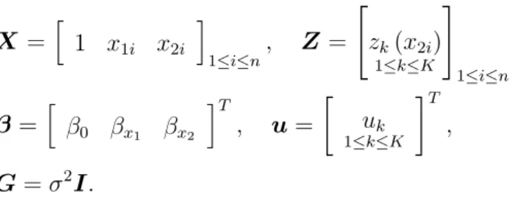
Lower-case Roman and Greek letters in boldface denote vectors whose entries are subscripts. For example, xdenotes an_×1 vector containingx1, . . . , xn. All vectors are column vectors. Upper-case Roman and Greek letters in boldface denote matrices. For example,X denotes am_×nmatrix containingnvectors of dimensionm_×1,x1, . . . ,xn.

R The set of real numbers.

Rn The set of real vectors of dimension n.

Rn×m The set of real matrices with n rows andm columns. T Transpose symbol for vectors and matrices.

(_·, . . . ,_·) Lists of scalars, vectors and matrices within round brackets are con-catenated vertically (vertical concatenation), e.g. a = (a1, . . . , an) is a column vector.

[_·, . . . ,_·] Lists of scalars, vectors and matrices within square brackets are concate-nated horizontally (horizontal concatenation), e.g. a = [a1, . . . , an] is a row vector. In addition, (a1, . . . ,an) =

aT 1, . . . ,aTn T . " aij 1≤i≤n # 1≤j≤m

Matrix with n rows and m columns or vector with n rows if m= 1. (a)_i orai The element in ith position of a vectora.

(A)_ij orAij The element in (i, j)th position of a matrix A.

diag (a) For a vector a_∈_Rn, diagonal matrix of size n_×n such that

diag (a) =        a1 0 · · · 0 0 a2 · · · 0 .. . ... . .. ... 0 0 _{· · ·} an        .

dg (A) For a square matrix A_∈_Rn×n_{, a vector of length} _n _{whose entries} corre-spond to the diagonal elements of A such that

dg               A11 A12 · · · A1n A21 A22 · · · A2n .. . ... . .. ... An1 An2 · · · Ann              

= (A11, A22, . . . , Ann).

(12)

1 An appropriately-sized vector or matrix of ones.

ei An appropriately-sized vector of zeros, except the ith value which is 1.

I An appropriately-sized identity matrix.

ab The element-wise multiplication of vectors a,b _∈ _Rn_{, that is,} (a1b1, . . . , anbn).

a/b The element-wise division of vectorsa,b_∈_Rn, that is, (a1/b1, . . . , an/bn). f(x) Univariate function f : _R _→ _R of a vector x _∈ _Rn such that f(x) =

(f(x1), . . . , f(xn)).

ka_k Vector 2₋norm of a vector a_∈_Rn _{such that} _k_a_k_{= (}Pn

i=1a 2 i)

1/2 . tr (A) The trace of the matrix A.

|A_| The determinant of the matrix A.

A−1 The inverse matrix of the matrix A.

A_⊗B The Kronecker product of matrices A _∈ _Rn×m _and _B _∈

Rp×q, that is, the np_×mq matrix defined by [aijB]₁≤i≤n,1≤j≤m.

AB The element-wise multiplication of matrices A,B _∈ _Rn×m_{, that is, the} n_×m matrix defined by [aijbij]₁_≤_i_≤_n,1_≤_j_≤_m.

vec (A) For a square matrix A _∈ _Rn×m, the nm_×1 vector obtained by stack-ing the columns of A underneath each other in order from left to right (vectorization) such that

vec (A) = (A11, . . . , An1, A12, . . . , An2, . . . , A1m, . . . , Anm).

vec−_n_×1_m(a) For a vector a _∈ _Rnm_{, the} _n _× _m _matrix _A _{formed from listing the} entries of a in a column-wise fashion in order from left to right, such that vec (A) =a; if the subscript is not specified, a _∈ _Rn2 and A is of size n_×n.

vech (A) For a symmetric matrix A_∈_Rn×n_{, the} _n_(n_{+ 1)}_/2_×_{1 vector obtained} by vectorizing only the lower triangular part of A (halph-vectorization) such that

vech (A) = A11, . . . , An1, A22, . . . , An2, . . . , A(n−1)(n−1), An(n−1), Ann

. vech−1(a) For a vector a _∈_Rn(n+1)/2, the n_×n symmetric matrix A whose lower

triangular part is formed from listing the entries of a in a column-wise fashion in order from left to right such that vech (A) = a.

Dn For a symmetric matrix A ∈ Rn×n, the duplication matrix of order n and size n2 _×_n_(n_{+ 1)}_{/2 containing all zeroes and ones such that}

Dnvech (A) = vec (A).

D+_n For a duplication matrix of order n, Dn, and a symmetric matrix

A_∈ _Rn×n_{, the} _{Moore–Penrose inverse} _D+

n ≡ D T nDn

−1

DT_n such that

(13)

blockdiag 1≤i≤d

(Ai) For matrices Ai ∈ Rni×mi, 1 ≤ i ≤ d, a matrix of size

Pd

i=1ni ×

Pd

i=1mi such that

blockdiag₁_≤_i_≤_d(Ai)≡        A1 O · · · O O A2 · · · O .. . ... . .. ... O O _{· · ·} Ad        . stack 1≤i≤d(Ai) For matrices Ai ∈R ni×m_{, 1}≤ _i≤_{d, a matrix of size} Pd i=1ni×m such that stack1≤i≤d(Ai)≡     A1 .. . Ad     .

I(x) Indicator variable, which takes the value 1 if xis true and 0 other-wise.

φ(x) Density function of a standard normal distributed random variable x.

Φ (x) Cumulative distribution function of a standard normal distributed random variable x.

o(_·) Forf andg real valued functions, both defined on some unbounded set of real positive numbers and g(x) strictly positive for all large enough values of x,f(x) = o(g(x)) as x_{→ ∞}if for every positive constant ε there exists a constant N such that _|f(x)_{| ≤} εg(x) for all x_≥N.

O(_·) Forf andg real valued functions, both defined on some unbounded set of real positive numbers and g(x) strictly positive for all large enough values of x, f(x) = O(g(x)) as x_{→ ∞}if and only if there exist a positive real number M and a real number x0 such that

(14)

(15)

List of Figures

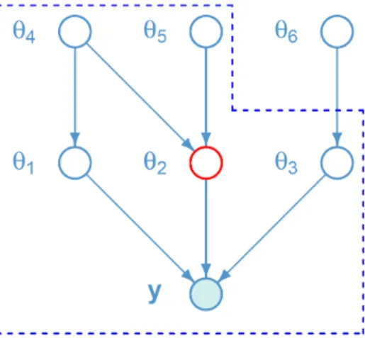
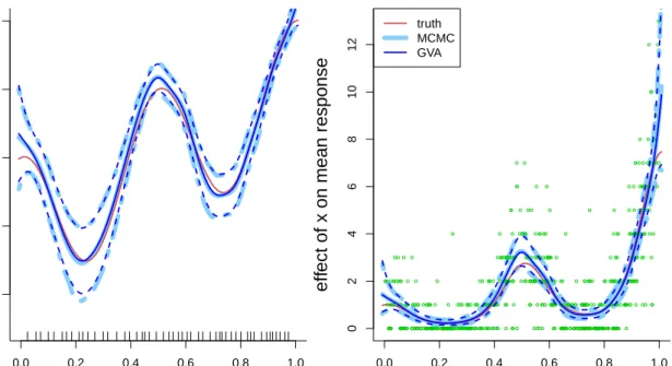
1.1 Directed acyclic graph corresponding to model (1.11). The six parame-ters (hidden nodes) are associated with circles. The shaded node y cor-responds to the obsered data (evidence node). The dashed line indicates the Markov blanket for θ2. . . 13 1.2 Factor graph for the regression model in (1.12) and restriction (1.13). . . 14 2.1 Left panel: mean estimate of f (solid line) and pointwise 95% credible

intervals (dashed lines) obtained via MCMC and GVA for the Poisson nonparametric regression model (2.7). The interior knots are drawn on the xaxis. The true f from which the data were generated is shown as a red solid line. Right panel: As for the left panel, but for exp (f) instead of f. The data are shown as circles. . . 36 2.2 Mean estimate of f (solid line) and pointwise 95% credible intervals

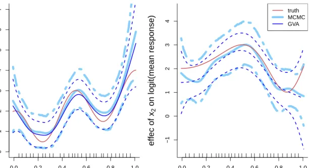
(dashed lines) with respect to x2, keeping x1 fixed to its mean, obtained via MCMC and GVA for the semiparametric logistic regression model (2.8). The interior knots are drawn on thexaxis. The truef from which the data were generated is shown as a red solid line line. . . 37 2.3 Left panel: mean estimate of f1 (solid line) and pointwise 95% credible

intervals (dashed lines) with respect to x1, keeping x2 fixed to its mean, obtained via MCMC and GVA for the logistic additive regression model (2.10). The interior knots are drawn on the x axis. The true function from which the data were generated is shown as a red solid line line. Right panel: As for the left panel, but for f2 plotted against x2, keeping

x1 fixed to its mean. . . 39 2.4 Plot of the data simulated according to (2.11). The symbol “+” indicates

the representative knots. . . 42 2.5 Left panel: mean estimate of f1 (solid line) and pointwise 95%

credi-ble intervals (dashed lines) with respect to x1, keeping x2 and spatial coordinates fixed to their mean, obtained via MCMC and GVA for the Poisson geoadditive model (2.12). The interior knots are drawn on the x axis. The true function from which the data were generated is shown as a red solid line line. Right panel: As for the left panel, but for f2 plotted against x2, keeping x1 and spatial coordinates fixed to their mean. . . 43 2.6 Mean square error comparisons. Left panel: comparison between GCV

and other methods involving Poisson non parametric models. Right panel: comparison between MCMC and other methods involving logistic additive models. . . 43

(20)

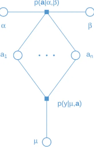
xviii List of Figures 3.1 Factor graph for the Pareto likelihood specification in (3.2) under the

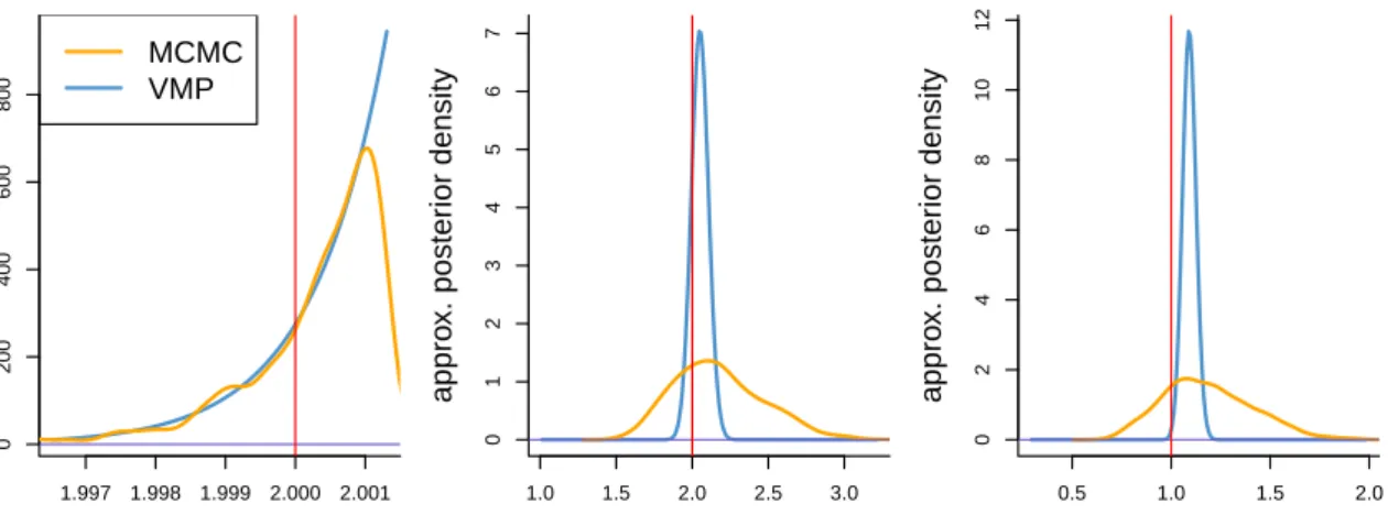
assumption in (3.3) with independent auxiliary variables a1. . . an. . . 49 3.2 VMP-approximate and MCMC posterior density functions for a dataset

simulated with parameters µ = 2, α = 1, β = 2. Vertical lines indicate the true values. . . 55 3.3 Loss function in support vector regression. . . 55 3.4 Factor graph for the support vector regression likelihood specification in

(3.14) under the assumption in (3.15) with independent auxiliary vari-ables a11. . . a1n and a21. . . a2n. . . 57 3.5 Directed acyclic graph for the support vector regression likelihood

speci-fication in (3.14). . . 59 3.6 Factor graph for the skewtlikelihood specification in (3.21) with

indepen-dentN(0,1) auxiliary variablesa11. . . a1nand independent Inverse-χ2(ν, ν) auxiliary variables a21. . . a2n under the assumption in (3.22) (left panel) and (3.24) (right panel). . . 63 3.7 Markov chain Monte Carlo samples (n= 1000) drawn viarstanfrom the

distribution

|a1|,1/√a2|rest for a skewtrandom sample withθ =µ= 0, σ = 1, ν = 1.5 and λ = (0.05,0.5,5,50), using the hyperparameters specified in Section 3.4.1. Sample correlations are also shown. . . 66 3.8 VMP-approximate and MCMC posterior density functions from a single

dataset of the simulation study. “VMP 1” and “VMP 2” respectively refer to Algorithms 3.4 and 3.5. VMP, variational message passing; MCMC, Markov chain Monte Carlo. Vertical lines indicate the true values. . . 69 3.9 Martin Marietta data: posterior density plots via MCMC and VMP. . . . 70 3.10 Study of data from Workinghours dataset. Left panel: factor graph

corresponding to the model in (3.25) under the product density restric-tion in (3.26). Right panel: approximate posterior mean (solid line) and pointwise 95% credible sets (dashed line) obtained via VMP, integrat-ing Algorithm 3.5; 20 observations whose “income/10” value exceeds 150 have been excluded from the plot. . . 72 4.1 Directed acyclic graph for the two-level Poisson and logistic response

mixed model in (4.7) and (4.17). . . 81 4.2 Factor graph for the two-level Poisson and logistic response mixed model

in (4.7) and (4.17). . . 87 4.3 Simulated two-level data with 36 schools, each having 200 students,

ac-cording to the Poisson multilevel model described in Section 4.5. Each panel contains the approximate posterior mean (solid line) and pointwise 95% credible intervals for the mean response. The true function from which the data were generated is shown as a red solid line. . . 90 4.4 Simulated two-level data with 100 schools, each having 500 students,

according to the logistic multilevel model described in Section 4.5. Each panel contains the approximate posterior mean (solid line) and pointwise 95% credible intervals for the mean response. The true function from which the data were generated is shown as a red solid line. . . 92

(21)

List of Tables

3.1 Average (standard deviation) accuracy from the simulation study. “VMP 1” and “VMP 2” refer to Algorithms 3.4 and 3.5 respectively. . . 69 4.1 Vectorspandscorresponding to thek = 8 normal scale mixture uniform

approximation of Monahan and Stefanski (1989). . . 84

(22)

(23)

List of Algorithms

3.1 The VMP inputs, updates and outputs of the Pareto random sample likelihood fragment assuming q(µ, α, β,a) = q(µ)q(α)q(β)Qn

i=1q(ai). . 54 3.2 The VMP inputs, updates and outputs of the support vector regression

likelihood fragment assuming q(θ,a1,a2) = q(θ)

Qn

i=1q(a1i)q(a2i). . . . 58 3.3 MFVB coordinate ascent procedure to obtain the parameters in the

opti-mal densities q∗(θ),q∗(a1) and q∗(a2) for the support vector regression model assuming q(θ,a1,a2) = q(θ)Qn

i=1q(a1i)q(a2i). . . 61 3.4 The VMP inputs, updates and outputs of the skew t likelihood fragment

assuming q(θ, σ2_{, λ, ν,}_a

1,a2) = q(θ)q(σ2)q(λ)q(ν)

Qn

i=1q(a1i)q(a2i). . 65 3.5 The VMP inputs, updates and outputs of the skew t likelihood fragment

assuming q(θ, σ2_{, λ, ν,}_a

1,a2) = q(θ)q(σ2)q(λ)q(ν)Qn_i=1q(a1i, a2i). . . 68 4.1 (Nolanet al., 2018)TheSolveTwoLevelSparseMatrixalgorithm for

solv-ing the two-level sparse matrix problem x=A−1a and sub-blocks ofA−1

corresponding to the non-zero sub-blocks of A. The sub-block notation is given by (4.2) and (4.3). . . 78 4.2 (Nolan et al., 2018) SolveTwoLevelSparseLeastSquares for solving the

two-level sparse matrix least squares problem: minimise _kb₋B x_k2 _in _x

and sub-blocks of A−1 corresponding to the non-zero sub-blocks of A =

BTB. The sub-block notation is given by (4.2), (4.3) and (4.5). . . 80 4.3 QR-decomposition-based streamlined algorithm for obtaining mean field

variational Bayes approximate posterior density functions for the param-eters in the two-level Poisson mixed model (4.7) with product density restriction (4.10). . . 93 4.4 QR-decomposition-based streamlined algorithm for obtaining mean field

variational Bayes approximate posterior density functions for the param-eters in the two-level logistic mixed model (4.17) with product density restriction (4.10). . . 94

(24)

xxii List of Tables 4.5 (Nolan et al., 2018) The TwoLevelNaturalToCommonParameters

algo-rithm for conversion of a two-level reduced natural parameter vector to its corresponding common parameters. . . 95 4.6 The inputs, updates and outputs of the matrix algebraic streamlined

Pois-son likelihood fragment for two-level models. . . 96 4.7 The inputs, updates and outputs of the matrix algebraic streamlined

(25)

(26)

(27)

Introduction

“Far better an approximate answer to the right question, which is often vague, than anexact answer to the wrong question, which can always be made precise.”

John W. Tukey1_{, 1915 – 2000}

Overview

The rapid growth of information has revolutionized the concept of data analysis and the instruments for handling data. In some cases, the amount of data to store has grown so much that standard computer memory is unable to manage such a large volume. This gives a new impulse to engineering research on new data processing technologies. In a similar manner, the celerity of processing information in recent years has motivated researchers and practitioners to develop and employ faster data analysis techniques in lieu of conventional methods whose running time does not match practical requirements. This big data revolution encourages the start of new research threads in statistics and, in the same spirit, is the drive behind this thesis. Specifically, the thesis focuses on the development and assessment of variational approximation methods for statistical inference and fitting problems from both likelihood based and Bayesian perspectives.

Variational approximations are a class of techniques for making approximate deter-ministic inference for complex statistical models. The name derives from the mathe-matical discipline of variational calculus, since the approximation is obtained from the optimization of a functional over a class of density functions on which that functional depends. Now part of conventional computer science methodology concerning elaborate problems such as natural language processing, speech recognition, document retrieval, genetic linkage analysis, computational biology, computational neuroscience, computer vision and robotics, variational approximations are finding a growing presence in statis-tics. However, much of the mainstream literature on variational approximations uses

1_{See Tukey (1962).}

(28)

2

terminology, notation, and examples from computer science rather than statistics. An introduction to the topic from a mere statistical perspective is contained in Ormerod and Wand (2010), that, in turn, refer to Jordan et al.(1999), Jordan (2004), Tittering-ton (2004), and Bishop (2006, Chapter 10) for summaries of variational approximations. Teschendorff et al. (2005), McGrory and Titterington (2007) and McGroryet al. (2009) are cited as works about variational approximation methodology for particular appli-cations, while Hall et al. (2002) and Wang and Titterington (2006) as references about the statistical properties of estimators obtained via variational approximation. Addi-tionally, a description of variational approximations as a machine learning method for approximating probability densities is included in Wainwright and Jordan (2008). A more recent reference, Blei et al. (2017), provides an exhaustive overview on varia-tional inference specifically addressed to statisticians. Particular emphasis is placed on the popular stochastic variational inference methodology (Hoffman et al., 2013), which scales variational inference to large datasets using stochastic optimization (Robbins and Monro, 1951).

Bleiet al.(2017) also assert that the development of variational techniques, initially for Bayesian inference, followed two parallel, yet separate, tracks. Peterson and Ander-son (1987) describe presumably the first variational procedure for a particular model, a neural network. Their article, in connection with some intuitions from statistical me-chanics (Parisi, 1988), brought to the flowering of variational inference procedures for a wide class of models. In parallel, a variational algorithm for a similar neural network model was proposed in Hinton and Van Camp (1993).

Though the theory around variational inference is not growing at the same speed as the methodology, there are several threads of research that prove theoretical guarantees of variational approximations. References are given in Section 5.2 of Blei et al. (2017). Additional results on asymptotic properties are included in Wang and Blei (2018) and Zhang and Gao (2018).

Variational approximations find application in both likelihood based and Bayesian inference problems. However, their use in the literature is far more widespread for Bayesian inference, where intractable calculus abounds and where they provide fast, de-terministic alternatives to Monte Carlo methods. The idea behind this methodology is to first propose a family of densities in the integral of interest and then to find the member of that family which is closest to the target density. In the standard version of varia-tional approximations the approximating density produces a lower bound and closeness is measured by Kullback–Leibler divergence (Kullback and Leibler, 1951). Nevertheless, not all variational approximations fit within the Kullback–Leibler divergence framework.

(29)

Introduction 3 Another variety are what might be called tangent transform variational approximations since they are based on tangent-type representations of concave and convex functions (e.g. Jordan et al., 1999; Ormerod and Wand, 2010, Section 3). This thesis is concerned with the first type of variational approximations to which we refer as density transform

approach. For sake of completeness, Wainwright and Jordan (2008) emphasized that any inferential procedure that uses optimization and alternative divergence measures to approximate a density can be named “variational inference”. This includes methods such as expectation propagation (Minka, 2001),belief propagation (Yedidia et al., 2001) or even the Laplace approximation.

The essence of the density transform variational approach is to provide an approxi-mation which is derived from a lower bound that is more tractable than the likelihood function. Tractability is enhanced by restricting the approximating density to a more manageable class of densities. The most common restrictions are:

(a) the approximating density is a member of a parametric family of density functions; (b) the approximating density factorizes as a product of densities according to a

par-tition of the set of parameters.

Note that (b) represents a type of nonparametric restriction since the product form is the only assumption being made. Restriction (b) produces the so-called mean field

approximation, whose roots are in statistical physics (e.g. Parisi, 1988). The term varia-tional Bayes has become commonplace for approximate Bayesian inference under prod-uct density restrictions. More recently, Wand (2017) reviseted mean field variational Bayes, with a focus on semiparametric regression, working with an approach known as

variational message passing (Winn and Bishop, 2005). This approach has the advan-tage that the algorithms it generates are amenable to modularization and extension to arbitrarily large models via the notion of factor graph (Frey et al., 1998) fragments.

Main contributions of the thesis

This thesis is developed around Kullback–Leibler-based variational methodologies that employ the restrictions (a) and (b) mentioned above, the former in frequentist settings, the latter for Bayesian inference. Specifically, the parametric restriction (a) is applied as a strategy for fitting generalized linear mixed models with general de-sign matrices, following the framework established in Ormerod and Wand (2012). The approach, named Gaussian variational approximations, consists in approximating the distribution of random effects vectors, conditional on the responses, with a Gaussian

(30)

4

density chosen to minimize a variational lower bound on the model likelihood func-tion. Our contribution lies in exposing Gaussian variational approximations as a fast and effective alternative to more widely used inference methods such as, for instance, penalized quasi likelihood or generalized cross-validation. Recently, Hui et al. (2018) have investigated the use of Gaussian variational approximations for generalized additive models. However, their approach puts emphasis on the penalty parameter estimation which in our formulation may arise as an outcome of the optimization problem and their optimization strategy is structured in a different way. Furthermore they get rid of a residual integration step still present in the variational lower bound for Bernoulli models by creating a second lower bound of the initial lower bound, while we prefer a fast and more accurate route with numerical integration.

The second part of the thesis is concerned with the nonparametric restriction (b) and the so called mean field variational Bayes methodology under the variational mes-sage passing perspective for factor graph fragments. We extend the work contained in McLean and Wand (2018) to accommodate additional elaborate likelihood fragments. The modularity of variational message passing permits relatively simple extensions to more complicated scenarios in such a way that, for instance, semiparametric regression models can be handled using factor graph fragments. Extension to arbitrarily large models is guaranteed by algorithm updates that are based on natural parameters and sufficient statistics of exponential family densities. Our practical implementations of variational algorithms employ factorised approximating posteriors and priors that be-long to the conjugate-exponential families, making the required integrals tractable.

Furthermore, we present explicit algorithms to implement streamlined variational inference for two-level non-normal response models. The algorithms take advantage of the sparse matrix results presented in Nolan et al. (2018) and are part of a framework which is prone to extension to high-level random effects models. Scalability for large datasets also benefits of the streamlined variational message passing approach.

The present thesis is organized in the following way. Chapter 1 defines the set-tings for the variational approximations methodology under consideration. A broader overview on variational inference techniques and some references to theoretical results are also provided. Details on semiparametric regression via O’Sullivan penalized splines (O’Sullivan, 1986) and the generalized linear model formulation through general design matrices are also provided.

Chapter 2 is dedicated toGaussian variational approximations. In detail, Poisson and binomial response models with nonparametric and additive structures are considered.

(31)

Introduction 5 Inference and confidence interval construction are easily derived from the estimated ap-proximating Gaussian density. Results are then compared to those obtained via classical fast estimation methods and good overall performances in terms of estimation time and inferential properties are observed. Issues involving the lower bound optimization are also investigated. Furthermore, the settings for fitting geoadditive models as an example of application to generalized linear mixed models with spatial structures are described. Each subsection of Chapter 3 develops variational algorithms catered to a particu-lar likelihood fragment. Three likelihood fragments, including Pareto random sample, support vector regression and skew t regression are explored. For the skew t case, we also investigate how various auxiliary random variable representations of the likelihood impact the variational approximating results. The response likelihoods are re-expressed in terms of auxiliary variables and more common distributions to avoid numerically in-tractable steps. As a drawback, we show that such a reparametrization may introduce strong posterior dependence among variables which is hard to capture with simple forms of approximating densities.

In Chapter 4 we develop fast variational algorithms for fitting and inference in mixed models, where all algorithmic updates are available in closed form. The centrepieces for Chapter 4 are streamlined variational algorithms for fast and memory efficient fitting and inference in large two-level Bayesian random effects models with Poisson and Binomial responses.

The probability distributions used in the thesis are displayed in Appendix A. The rest of the Appendix reflects the structure of main chapters and essentiallyv complements derivations and computational steps.

All the numerical analyses appearing in this thesis are supported by a comparison with Markov chain Monte Carlo, which provides our benchmark for assessing variational approximation performances.

(32)

(33)

Chapter 1 Variational inference

1.1 Density transform variational approximations

The class of variational approximations contains a wide range of techniques for determin-istic approximate inference. In the present thesis, the variational approximation meth-ods under consideration refer to the most common variant, known as density transform approach, according to the classification of Ormerod and Wand (2010). This method involves approximation of conditional distributions of interest or posterior densities by other densities that minimize the divergence to the densities of interest and for which inference is more tractable. We describe these concepts more in detail with an example in the Bayesian setting. The following illustration easily extends to variational inference for frequentist models.

Consider a generic Bayesian model with parameter vectorθ, parameter space Θ and observed data vector y, where, for simplicity, we assume that both the random vectors are continuous. Bayesian inference is concerned with the posterior density function

p(θ_|y) = p(y,θ) p(y) ,

where p(y,θ) is the joint density of y and θ, and p(y) is known as the marginal likelihood or model evidence in the computer science literature on variational approx-imations. Given an arbitrary density function q defined over Θ, the logarithm of the

(34)

8 Section 1.1 -Density transform variational approximations

marginal likelihood satisfies logp(y) = logp(y) Z q(θ)dθ = Z q(θ) log p(y,θ)/q(θ) p(θ_|y)/q(θ) dθ = Z q(θ) log p(y,θ) q(θ) dθ+ Z q(θ) log q(θ) p(θ_|y) dθ (1.1) ≥ Z q(θ) log p(y,θ) q(θ) dθ. (1.2)

Note that the second integral on the right hand side of (1.1) is the Kullback–Leibler divergence between q and p(θ_|y),

KL_{q(θ) _kp(θ_|y)_}= Z q(θ) log q(θ) p(θ_|y) dθ, (1.3)

which is non-negative for all densities q, with equality arising if and only if q(θ) = p(θ_|y). This gives the inequality (1.2) and a lower bound p(y;q) on the marginal likelihood p(y)_≥p(y;q) = exp Z q(θ) log p(y,θ) q(θ) dθ. (1.4)

Maximization of p(y;q) is equivalent to minimization of the Kullback–Leibler diver-gence between q(θ) and p(θ_|y) and may provide an alternative approach to the direct optimization of the marginal likelihood. The new maximization problem consists in finding the optimal approximating density in terms of Kullback–Leibler divergence that approximates the posterior density function.

The lower bound (1.4) can be also obtained via the Jensen’s inequality, if renouncing to quantify the gap between p(y) and p(y;q) (e.g. Jordan et al., 1999).

The whole idea behind this approach is to propose an approximation of the posterior density p(θ_|y) by a q(θ) for which p(y;q) is more tractable thanp(y). Tractability is achieved by restricting q(θ) to a more manageable class of densities. As described in the previous chapter, the two common restrictions are:

(a) q(θ) is a member of a parametric family of density functions; (b) q(θ) factorizes as QM

i=1qi(θi), for some partition{θ1, . . . ,θM} of θ.

Depending on the model at hand, both restrictions can have minor or major impacts on the approximation performances in terms of accuracy.

An approximation based on the parametric restriction (a) is named Gaussian vari-ational approximation (GVA) whenever the approximating density q(θ) is assumed to

(35)

Chapter 1 - Variational inference 9 be within the family of Gaussian densities. Section 1.2 provides a brief description of GVA.

Also known as mean field approximation in Bayesian statistics, the product density form in case (b) is the only assumption being made and represents a type of nonpara-metric restriction. Restricting q to a subclass of product densities gives rise to explicit solutions to the optimization problem for each product component in terms of the others and, in turn, leads to an iterative scheme to obtain the simultaneous solutions which is known as mean field variational Bayes (MFVB). Variational message passing (VMP) is a prescription for obtaining mean field variational Bayes (MFVB) approximations to posterior density functions that allows for modularization and extension to arbitrarily large models. Both the MFVB and VMP perspectives are treated in Section 1.3.

Section 1.4 contains a concise review of early references on the mean field methodol-ogy and a glance at the class of message passing algorithms.

Section 1.5 provides some references to the theory of variational approximations that present connections with the methods considered in this thesis.

Finally, Section 1.6 is dedicated to an accessory but recurrent topic in the present thesis, that is, semiparametric regression. In particular, the mixed model representation of semiparametric regression models facilitates variational approximate inference under both restrictions above.

1.2 Gaussian variational approximations

Nontrivial frequentist examples where an explicit solution arises by applying the product density methodology are not known. On the other hand, restricting the approximating density to be part of a parametric family of density functions may lead to effective variational approximation strategies.

Frequentist models that stand to benefit from variational approximations are those for which specification of the likelihood involves conditioning on a vector of latent vari-ables u. Given a vector of observed data y, the log-likelihood of the model parameter vector θ takes the form

`(θ) = logp(y;θ) = log Z p(y_|u;θ)p(u;θ)du, and ˆ θ = argmax θ `(θ) is the maximum likelihood estimate of θ.

(36)

10 Section 1.3 -Mean field variational approximations

For some statistical models, the log-likelihood`(θ) may not be available in a closed form because of analytically intractable integration. In such a context, variational ap-proximations can provide a more tractable approximation in replacement of the original optimization problem, depending on the forms of p(y_|u;θ) and p(u;θ).

In this context, the auxiliary functionqis a density of the latent variableu. Suppose to restrict qto a parametric family of densities _{q(u;ξ) :ξ_∈Ξ_}, where ξ is a vector of

variational parameters. Then a log-likelihood lower bound `(θ,ξ;q) = Z q(u;ξ) log p(y,u;θ) q(u;ξ) du (1.5)

can be derived, as shown for the Bayesian counterpart (1.2). The new maximization problem over the model parameters θ and the variational parametersξ

ˆ

θ,ξˆ= argmax

θ,ξ

`(θ,ξ;q)

is the set-up for variational approximate inference and GVA, when theq(u;ξ) is chosen to be a family of normal densities. The vector ˆθ is a variational approximation to the maximum likelihood estimate ˆθ. Estimated standard errors can be obtained by plugging in ˆθforθ and ˆξforξin the variational approximate Fisher information matrix arising from replacement of`(θ) by`(θ,ξ;q) and the corresponding Hessian matrix (e.g. Ormerod and Wand, 2012).

1.3 Mean field variational approximations

Variational message passing is an approach to variational Bayes approximate inference that allows modularization through the notions of factor graphs and message passing. According to a factor graph message passing approach (e.g. Minka and Winn, 2008, Appendix A), calculations only need to be performed once for a particular fragment and can be integrated with other fragments to construct inference engines for arbitrarily large models.

A mean field variational approximation q∗(θ) to p(θ_|y) is the minimizer of the Kullback–Leibler divergence (1.3) subject to a product density restriction, or mean field restriction, q(θ) = M Y i=1 q(θi), (1.6)

(37)

Chapter 1 - Variational inference 11 where _{θ1, . . . ,θM} is some partition of θ. It can be shown (e.g. Ormerod and Wand, 2010, Section 2.2) that the optimal q-density functions satisfy

q∗(θi)∝exp Eq(θ\θi)logp(y,θ) , 1≤i≤M, (1.7) or, alternatively, q∗(θi)∝exp Eq(θ\θi)logp(θi|y,θ\θi) , 1≤i≤M, (1.8)

where θ_\θi denotes the entries ofθ with θi omitted and the distribution p(θi|y,θ\θi) is known as full conditional density function. The previous expression gives rise to the MFVB iterative scheme for obtaining the optimal density functions q∗(θi). A listing of such an algorithm is provided, for instance, in Ormerod and Wand (2010). Alternatively, optimization may be performed via a message passing algorithmic approach for mean field approximation (VMP), which is limited to conjugate exponential family models (Winn and Bishop, 2005).

When expectation steps appearing in algorithm updates require evaluation of definite integrals that do not admit analytic solutions or easily manageable analytic solutions, univariate quadrature schemes may be considered. The trapezoidal rule is a simple and effective quadrature approach, whose accuracy arbitrarily improves by increasing the number of trapezoidal elements. If the integral is over an infinite or semi-infinite region, rather than a compact interval, it is important to define the effective support of the integrand function to guarantee accurate computation. Attention is necessary to avoid overflow and underflow issues concerning the application of the trapezoidal rule.

1.3.1 Coordinate ascent mean field variational Bayes

Expression (1.7) gives rise to a conceptually simple coordinate ascent algorithm. First, initialize q(θ1), . . . , q(θM). Then cycle

qi(θi)←− expEq(θ\θi)logp(y,θ) R exp Eq(θ\θi)logp(y,θ) dθi ,

for each 1 _≤i_≤M, until the increase in the lower bound on the marginal log-likelihood logp(y;q) =Eq(θ){logp(y,θ)−logq(θ)} (1.9) is negligible. The optimalq_i∗(θi) densities are obtained at convergence. The←−symbol means that the function ofθi on the left-hand side is updated according to the expression

(38)

on the right-hand side; multiplicative factors not depending on θi can be ignored. The expressions containing such a symbol are technically named “updates”.

The termEq(θ){logq(θ)}in (1.9) is the so calledentropy of the density functionq(θ). Boyd and Vandenberghe (2004) use convexity properties to show that convergence to at least a local optimum is guaranteed. In fact, the MFVB scheme is basically interpretable as a generalisation of the expectation-maximisation (EM) approach (Chappell et al., 2009).

In presence of conjugacy with priors, one may take advantage of the optimal form (1.8) and associate the q∗(θi)s to recognizable density families. Then the optimization procedure reduces to updating parameters in the q∗(θi) family.

Directed acyclic graph (DAG) representations of Bayesian models are very useful when deriving the optimal q-densities formulated as (1.8). In detail, DAGs yield sub-stantial benefits to MFVB schemes for large models taking advantage of an important probabilistic concept, namely the Markov blanket theory. For each node on a proba-bilistic DAG, the conditional distribution of the node given the rest of the nodes is the same as the conditional distribution of the node given its Markov blanket (Dechter and Pearl, 1988), whose definition is provided in the exemplification below. In the Bayesian models considered here this implies

p(θi|y,θ\θi) =p(θi|Markov blanket of θi). It follows that (1.8) simplifies to

q∗(θi)∝exp

Eq(θ\θi)logp(θi|Markov blanket of θi) , 1≤i≤M. (1.10)

This is known as thelocality property of DAGs. For large DAGs, this property produces considerable algebraic benefits. Such a result means that determination of the required full conditionals involves only a series of local calculations on the DAG. In particular, it shows that the q∗(θi)s require only local calculations on the models DAG. We explain this concept with an elementary graphical example.

Consider the following hierarchical Bayesian model similar to the exemplification provided in Wand et al. (2011):

y_|θ1, θ2, θ3 _∼p(y_|θ1, θ2, θ3),

θ1|θ4 ∼p(θ1|θ4), θ2|θ4, θ5 ∼p(θ2|θ4, θ5), θ3|θ6 ∼p(θ3|θ6) indep., θ4 ∼p(θ4), θ5 ∼p(θ5), θ6 ∼p(θ6) indep.,

(39)

Chapter 1 - Variational inference 13 where y is the observed data vector and θ1, . . . , θ6 are model parameters. Figure 1.1

Figure 1.1: Directed acyclic graph corresponding to model (1.11). The six param-eters (hidden nodes) are associated with circles. The shaded node y corresponds to the obsered data (evidence node). The dashed line indicates the Markov blanket for

θ2.

shows the directed acyclic graph representation of model (1.11). The θis, 1 ≤ i ≤ 6, are represented by open circles namedhidden nodes and the data vectory, theevidence node, is portrayed by a shaded circle. The arrows indicate conditional dependence relationships among the model random variables. A DAG can be interpreted as a

family tree in which each directed edge conveys a parent-child relationship between the associated nodes. For instance, the node θ2 is pointed by the arrow-heads departing from nodes θ4 and θ5, therefore θ2 is a child of the parent nodes θ4 and θ5. The nodes θ1 and θ3 are co-parents of node θ2 since they all have a common child, y. The Markov blanket of a node, sayθ2, is the set including the parents, co-parents and children nodes (θ1,θ3, θ4, θ5 and y) of that particular node, as displayed by the dashed line in Figure 1.1. Briefly, the Markov blanket of a node separates that node from the remainder of the graph and has a probabilistic interpretation known as locality property. Because of (1.10), q∗(θ2) depends on particular q-density moments of θ1, θ3, θ4 and θ5 but not on their distribution. Therefore changing, for example, the distributional assumptions on p(θ1_|θ4) will not affect the form of q∗(θ2).

The locality property of MFVB ensures that attention can be restricted to the sim-plest versions of the models of interest and in particular to the response distribution, knowing that the forms of the optimal densities preserve the same structure also in larger models. This property and the factor graph fragment perspective employed in variational message passing have motivated our focus on the simplest forms of likelihood fragments described in Chapter 3.

(40)

1.3.2 Variational message passing on factor graphs

Variational message passing arrives at variational Bayes approximation via message passing on an appropriate factor graph. A factor graph is a graphical representation of the argument groupings of a real-valued function. Consider, for example, the regression model

y_|β, σ2 _∼N Xβ, σ2I, β_∼N(µβ,Σβ),

σ2_|a_∼Inverse-χ2(1,1/a), a_∼Inverse-χ2 1,1/A2

,

(1.12)

where yis ann_×1 vector of response data and X is ann_×ddesign matrix. The d_×1 vectorµβ, thed×dcovariance matrixΣβandA >0 are user-specified hyperparameters.

A factor graph representation of this model based on the product density restriction q β, σ2, a=q(β)q σ2q(a) (1.13) is that of Figure 1.2.

p(β) β p(y|β,σ2) σ2 p(σ2|a) a p(a)

Figure 1.2: Factor graph for the regression model in (1.12) and restriction (1.13).

Each factor graph has a corresponding graphical representation based on nodes con-nected by edges. The word node is used for both a stochastic node θi, 1 _≤ i _≤ M, and a factor fj, 1≤ j ≤N. In detail, the shaded squares correspond to factors, which are single product components of the real-valued function. The unshaded circles are called stochastic nodes and refer to parameters expressing product dependencies in the approximating density. An edge connects a factor to the stochastic nodes included in that factor. Two nodes are neighbors of each other if they are joined by an edge. In Fig-ure 1.2, stochastic nodes β and σ2 are neighbors of the factor p(y_|β, σ2), for instance. We denote by neighbors (j) the θi indices connected to the jth factor.

Rather than using result (1.8), the VMP procedure is founded upon the notion of

messages passed between any two neighboring nodes, which are a particular function of the stochastic node that either sends or receives the message. Among the several variants of VMP in the literature, we follow the approach of Minka (2005), which is described in Section 2.5 of Wand (2017). The approach is here briefly summarized.

(41)

Chapter 1 - Variational inference 15 Let N be the number of factors. For each 1 _≤ i _≤ M and 1 _≤ j _≤ N, the VMP

stochastic node to factor message updates are mθi→fj(θi)←−

Y

j06=j:i∈neighbors₍j0₎ mf

j0→θi(θi) (1.14)

and the factor to stochastic node message updates have form mfj→θi(θi)←−exp

Efj→θi

logfj θneighbors(j) , (1.15) with Efj→θi denoting expectation with respect to the density function

Q i0∈neighbors(j)\{i}mfj→θ i0 (θi 0)m_θ i0→fj(θi 0) Q i0∈neighbors(j)\{i} R mfj→θ_i0 (θ_i0)mθ i0→fj(θi 0)dθ i0 . (1.16)

If neighbors (j)_{\ {}i_}=_∅, then the expectation in (1.15) can be dropped and the right-hand side of (1.15) is proportional tofj θneighbors(j)

. In general, the optimalq-densities are obtained from

q∗(θi)∝ Y j:i∈neighbors(j) m∗_f j→θi(θi), (1.17) where m∗_f

j→θi(θi) are the optimal messages at convergence. Formally, convergence of

the message updates may be assessed by monitoring at each iteration the lower bound of the marginal log-likelihood

logp(q;y) = M X i=1 Eq(θi){logq(θi)}+ N X j=1 Eq(θi){log (fj)},

where the first component is known as the entropy or differential entropy. In practice, derivation of the lower bound expression may be cumbersome when the approximating densitiesq(θi)s belong to non-standard exponential families. Alternatively, convergence may be determined tracking the parameters of the approximating densities. In the present thesis, we choose the latter strategy.

We also define the notation

η_f↔θ =ηf→θ+ηθ→f

for any natural parameter η, factor f and stochastic node θ, in support of Chapters 3 and 4. Natural parameters arise from the theory of exponential families described in Section A.2.1 of Appendix A.

(42)

16 Section 1.4 -Variational approximations and message passing

1.4 Variational approximations and message

pass-ing

One way to orient oneself inside the vast literature on variational approximations is to understand the physical interpretation of variational methods. Starting from the original concepts of mean field approximations derived in statistical physics, we contextualize the variational message passing approach inside a broader class of message passing algorithms.

1.4.1 The origins of mean field approximations

Peterson and Anderson (1987) describe what is arguably the first variational procedure for a particular model, a neural network. The mean field approximation has its roots in physics, where it is known as mean field theory. Later, it was then extended to inference in graphical models (e.g. Jordan et al., 1999; Attias, 1999). Subsequently, it gradually penetrated into conventional statistical literature (e.g. Teschendorff et al., 2005; McGrory and Titterington, 2007).

Parisi (1988) is usually cited in the statistics literature as a key reference to the origins of mean field theory in physics. The book treats statistical field theory and is built upon the principles of statistical mechanics, nevertheless it includes interesting analogies with statistics that we highlight here.

Statistical mechanics is involved with deriving thermodynamic properties of macro-scopic bodies starting from a description of the motion of micromacro-scopic components such as atoms, electrons, etc. Classical mechanics would approach this problem by defining a Hamiltonian system that describes the evolution of the dynamic physical system and initial conditions. Since this problem formulation concerning the physical system is par-ticularly complex, probabilistic methods are introduced. The problem can be treated in two steps:

(1) finding the probability distribution of the microscopic components in thermal equi-librium, for example, after a sufficiently long time;

(2) compute the macroscopic properties of the system given the microscopic proba-bility distribution.

For the rest of this subsection, we preserve some of the classic physics notation and terminology to convey the main concepts and maintain a direct reference to original sources such as Parisi (1988) and Yedidia et al. (2005).

(43)

Chapter 1 - Variational inference 17 Consider a system of N particles, each having a state xi. The overall state of the system x=_{x1, . . . , xN}has a correspondingenergy E(x). In thermal equilibrium, the probability of a state will be given by the Bolthanzmann Law

p(x) = 1 Z(T)e

−E(x)/T ,

whereT is the temperature andZ(T) is the normalization constant (partition function) Z(T) =X

x∈S

e−E(x)/T,

with S the space of all possible states xof the system. The Helmholts free energy FH of a system is

FH =−logZ.

Physicists have devoted considerable effort to developing techniques which give good ap-proximations toFH. The variational approach is based on a trial probability distribution b(x) and a corresponding variational free energy (Gibbs free energy)

F (b) = U(b)₋H(b), where U(b) is the variational average energy

U(b) = X

x∈S

b(x)E(x)

and H(b) is thevariational entropy

H(b) = ₋X x∈S b(x) logb(x). It follows that F (b) =FH + KL (bkp), where KL (b_kp) = X x∈S b(x) log b(x) p(x)

is the Kullback-Leibler divergence between b(x) and p(x), which drives the choice of the optimal trial probability distribution b(x). Since the Kullback–Leibler divergence is always non-negative, F (b) _≥ FH, with equality when b(x) = p(x). Minimizing the

(44)

18 Section 1.4 -Variational approximations and message passing

variational free energy F (b) with respect to the trial probability function b(x) can be intractable for largeN. A possible solution is to impose a mean field restriction to b(x) such that b(x) = N Y i=1 bi(xi),

which is analogous to the assumption on the approximating density at the base of statistical mean field algorithms.

1.4.2 Message passing algorithms

The literature on variational approximation methods is not limited to the approxima-tion by Kullback–Leibler divergence. Alternative divergences may be hard to optimize but give better approximations (Minka, 2005). Nevertheless, one general way to un-derstand this class of algorithms is to view their cost functions as the aforementioned free-energy functions from statistical physics (Yedidia et al., 2005; Heskes, 2003). From this viewpoint, each algorithm arises as a different way to approximate the entropy of a distribution, in a similar way as in Subsection 1.4.1.

Message passing is a method for fitting variational approximations including several variants, each minimizing a different cost function with different message equations. Minka (2005) presents a unifying view of message passing algorithms as a class of meth-ods that differ only by the divergence they minimize. From such a perspective, the ensemble of message passing techniques may include the following approaches:

• Loopy belief propagation (Frey and MacKay, 1998);

• Expectation propagation (Minka, 2001);

• Fractional belief propagation (Wiegerinck and Heskes, 2003);

• Power expectation propagation (Minka, 2004).

• Variational message passing (Winn and Bishop, 2005);

• Tree-reweighted message-passing (Wainwright et al., 2005).

Minka (2005) describes the behavior of different message-passing algorithms through the illustration of divergence measure properties, with a particular focus on the α-divergence, a generalization of the Kullback–Leibler divergence indexed byα_∈_R_{\ {}0; 1_}. Given a density p and an approximating density q, the α-divergence measure between

(45)

Chapter 1 - Variational inference 19 p and q is Dα(pkq) = R αp(x) + (1₋α)q(x)₋p(x)αq(x)1−α dx α(1₋α) .

This divergence measure corresponds to KL(q_kp) for α _→ 0 and KL(p_kq) when α _→1.

Wainwright and Jordan (2008) point out that also other deterministic algorithms, such as the sum-product algorithm (e.g. Kschischang et al., 2001) and semi-denite re-laxations based onLasserre sequences (e.g. Lasserre, 2001), can be couched within the variational methodology framework. Li and Turner (2016) propose a generalized varia-tional inference approach deriving a lower bound via the R´enyi divergence.

1.5 Theory

Research on the accuracy of the variational approximation is lacking in the computer science literature. This provides statistical sciences with an opportunity to develop interdisciplinary contributions with quantitative performance assessments. Research into the quality of the variational approximation for specific models is present in the statistical literature, but offers extensions towards several directions.

Wang and Titterington (2003) study the consistency properties of variational Bayesian estimators for mixture models of known densities. It was shown that, with probability 1, the proposed algorithm converges locally to the maximum likelihood estimator when iterations approach infinity. Wang and Titterington (2006) describe a general algorithm for computing variational Bayesian estimates and study its convergence properties for a normal mixture model.

Hall et al. (2011a) and Hall et al. (2011b) use a Gaussian variational approxima-tion to estimate the parameters of a simple Poisson mixed-effects model with a single predictor and a random intercept. They prove consistency of these estimates, provide rates of convergence and show asymptotic normality with asymptotically valid standard errors. Ormerod and Wand (2012) extend with heuristic arguments these results for the consistency of Gaussian variational approximations for more general generalized linear mixed models.

Wang and Blei (2018) describe frequentist consistency and asymptotic normality of variational Bayes methods. Specifically, they connect variational Bayes methods to point estimates based on variational approximations. Zhang and Gao (2018) study

(46)

20 Section 1.6 - Semiparametric regression

convergence rates of variational posterior distributions for nonparametric and high-dimensional inference, with a focus on the variational Bayes methodology.

Jordan (2004), Titterington (2004) and Bleiet al.(2017) indicate further sources for a comprehensive listing of other relevant literature on the accuracy of the variational approximation.

1.6 Semiparametric regression

Variational methods may be proposed as a fast and effective tool for handling semi-parametric regression models under both the frequentist and Bayesian perspectives. Furthermore, the notion of message passing can be used to streamline the algebra and computer coding for approximate inference in large Bayesian semiparametric regression models, taking advantage of sparse structures of design and covariance matrices. This motivates a brief overview of semiparametric models.

Parametric models such as linear, linear mixed, generalized linear or generalized lin-ear mixed models use a particular functional form of predictors to explain the mean response. Such parametric assumption may offer a simple and interpretable representa-tion of the relarepresenta-tionship between response and predictors but it might not be suitable for circumstances in which the mean response is scarcely interpretable as a known function of predictors.

Semiparametric regression extends classical parametric regression analysis to allow the treatment of nonlinear predictor components. This extension can be achieved through penalized basis functions such as, for instance, B-splines or Daubechies wavelets and random effects modelling analogous to the classical longitudinal and multilevel anal-ysis. Consequently, the general framework of mixed models offers a tailored infrastruc-ture also for fitting and inference of semiparametric regression models. Furthermore, in the Bayesian settings, semiparametric regression finds a corresponding directed acyclic graphical model representation which supports the derivation of MCMC and scalable MFVB algorithms.

The variational methodological studies and applications of this thesis concerning semiparametric regression make use of the mixed model representation and O’Sullivan splines, which are an immediate generalization of smoothing splines based on penal-ized B-splines basis functions (e.g. O’Sullivan, 1986; Green and Silverman, 1994). The classical smoothing splines involve a number of basis functions which approximately equals the sample size. A spline of order k is a continuous piecewise polynomial with

(47)

Chapter 1 - Variational inference 21 continuous derivatives up to orderk₋1. O’Sullivan penalised splines possess the attrac-tive feature of requiring remarkably fewer basis functions. Furthermore, their natural boundary conditions (e.g. Green and Silverman, 1994, p. 12), computational numerical stability and smoothness make them of particular interest in the spline-based semipara-metric literature as well as a reliable choice of basis for standard statistical software implementations.

Wand and Ormerod (2008) provide a detailed description of O’Sullivan penalised splines and their mixed model representation, including examples with R code. We briefly summarize the approach here with an example.

1.6.1 Semiparametric regression via O’Sullivan penalized splines

Consider the simple nonparameteric regression setting yi =f(xi) +εi, 1_≤i_≤n,

where (xi, yi) ∈ R×R and εis are random variables with E(εi) = 0 and variance σ2ε. Suppose we are interested in estimating f over the interval [a, b] containing thexis via a set of cubic B-spline basis functions Bx = [B1(x), . . . , BK+4(x)], for K ≤ n. The corresponding knot sequence is defined by a=κ1 =κ2 =κ3 =κ4 < κ5 <_{· · ·}< κK+4 < κK+5 = κK+6 = κK+7 = κK+8 = b, where the actual values of the additional knots beyond the boundary are arbitrary and it is customary to make them all the same and equal toaandb, respectively (e.g. Hastieet al., 2009, Chapter 5). We require a function that minimizes the penalized residual sum of squares (PRSS)

P RSS(f, λ) = n X i=1 {yi−f(xi)} 2 +λ Z b a f00(x)2dx, (1.18) The expression λRb a f 00

(x)2dxis the so-calledpenalty term because it penalizes fits that are too rough, thus yielding a smoother result. The amount of smoothing is controlled by λ > 0, where λ is usually referred to as a smoothing parameter. The case λ = 0 corresponds to the unconstrained problem. The solution to (1.18) is the O’Sullivan penalized spline f(x) =Bν and thus (1.18) can be rewritten as

(48)

22 Section 1.6 - Semiparametric regression

where B is the design matrix with Bik = Bk(xi) and Ω is the penalty matrix with Ω_kk0 =Rb

aB 00 k(x)B

00

k0 (x)dx. Straightforward algebraic manipulation leads to the follow-ing O’Sullivan penalized spline with a solution to (1.19) such that

ˆ

f(x) =Bνˆ and νˆ = BTB+λΩ−1

BTy. (1.20)

In the special case in which the interior knots coincide with the xis, assumed distinct, ˆ

f(x) corresponds to the cubic smoothing spline arising as the minimizer of (1.18) (e.g. Schoenberg, 1964). These results also generalize to order m smoothing splines. Com-putation of the design matrix B is straightforward and is readily available in the R

environment. However, computation of the penalty matrix Ω can be challenging. In Section 6 of Wand and Ormerod (2008), an exact matrix expression forΩ is derived by applying the Simpson’s rule over each of the inter-knot differences, given as

Ω=B˜00T diag (ω) ˜B00,

where ˜B00 is the 3 (K+ 7)_×(K+ 4) matrix with (i, j)th entry B00_j (˜xi), ˜xi is the ith entry of the vector

˜ xi = κ1, κ1+κ2 2 , κ2, κ2+κ3 2 , κ3, . . . , κK+7, κK+7+κK+8 2 , κK+8 ,

and ω is the 3 (K + 7)_×1 vector given by

ω = 1 6(∆κ)1, 2 3(∆κ)1, 1 6(∆κ)1, 1 6(∆κ)2, 2 3(∆κ)2, 1 6(∆κ)2, . . . , 1 6(∆κ)K+7, 2 3(∆κ)K+7, 1 6(∆κ)K+7 ,

where (∆κ)_k =κk+1−κk,1≤k ≤K+ 7. A common default choice for the number of knots is

K = min (nU/4,35), (1.21)

wherenUis the number of uniquexisand the distribution of knots can either be quantile-based or equally spaced (e.g. Ruppert et al., 2003). In the next section we show how the O’Sullivan penalized splines can be expressed within the mixed model and Bayesian hierarchical model framework.

The positive penalization constant λ in (1.18) remains unspecified. An appropriate value for the constant λ trades the loss term given by the residual sum of squares against the penalty term. As pointed out in Luts and Ormerod (2014) this restricts