On the Machining Dynamics of Turning and Micro-milling Processes

(1)

ON THE MACHINING DYNAMICS OF TURNING AND MICRO-MILLING PROCESSES

A Thesis by

ERIC BEN HALFMANN

Submitted to the Office of Graduate Studies of Texas A&M University

in partial fulfillment of the requirements for the degree of MASTER OF SCIENCE

August 2012

(2)

(3)

ON THE MACHINING DYNAMICS OF TURNING

AND MICRO-MILLING PROCESSES

A Thesis by

ERIC BEN HALFMANN

Submitted to the Office of Graduate Studies of Texas A&M University

in partial fulfillment of the requirements for the degree of MASTER OF SCIENCE

Approved by:

Chair of Committee, C. Steve Suh Committee Members, Alan Palazzolo

Jyhwen Wang Wayne Hung Head of Department, Jerald A. Caton

August 2012

(4)

ABSTRACT

On The Machining Dynamics of Turning and Micro-milling Processes. (August 2012)

Eric Ben Halfmann, B.S., Lamar University Chair of Advisory Committee: Dr. C. Steve Suh

Excessive vibrations continue to be a major hurdle in improving machining efficiency and achieving stable high speed cutting. To overcome detrimental vibrations, an enhanced understanding of the underlying nonlinear dynamics is required. Cutting instability is commonly studied through modeling and analysis which incorporates linearization that obscures the true nonlinear characteristics of the system which are prominent at high speeds. Thus to enhance cutting dynamics knowledge, a comprehensive nonlinear turning model that includes tool-workpiece interaction is experimentally validated using a commercial laser vibrometer to capture tool and workpiece vibrations. A procedure is developed to use instantaneous frequency for experimental time-frequency analysis and is shown to thoroughly characterize the underlying dynamics and identify chatter.

For the tests performed, chatter is associated with changing spectral components and bifurcations which provides a view of the underlying dynamics not experimentally observed before. Validation of the turning model revealed that the underlying dynamics observed experimentally are accurately captured, and the coupled tool-workpiece chatter

(5)

vibrations are simulated. The stability diagram shows an increase in the chatter-free limit as the spindle speed increases until 1500rpm where it begins to level out. At high speeds the workpiece dominates the dynamics, and excessive workpiece vibrations create another stability limit to consider. Thus, workpiece dynamics should not be neglected in analyses for the design of machine tools and robust control laws.

The chip formation mechanisms and high speeds make micro-milling highly non-linear and capable of producing broadband frequencies that negatively affect the tool. A nonlinear dynamic micro-milling model is developed to study the effect of parameters on tool performance through spectral analysis using instantaneous frequency. A lumped mass-spring-damper system is assumed for modeling the tool, and a slip-line force mechanism is adopted. The effective rake angle, helical angle, and instantaneous chip thickness are accounted for. The model produced the high frequency force components seen experimentally in literature. It is found that increasing the helical angle decreased the forces, and an increase in system stiffness improved the dynamic response. Also, dynamic instability had the largest effect on tool performance with the spindle speed being the most critical parameter.

(6)

ACKNOWLEDGEMENTS

I would like to thank God for my many blessings and for the opportunity to attend Texas A&M. I am very appreciative of my fiancé for the never-ending love and support she provides me. I would like to thank my family, especially my parents, for the enduring love, support, guidance, and prayers throughout my life providing me with the foundation needed to be successful.

I would also like to express my sincere gratitude to my academic advisor, Dr. C. Steve Suh, for dedicating the time to mentor me and help me develop the professional and critical thinking skills needed to effectively approach and solve a problem. His continuous guidance and support provided me with a fulfilling research experience and an enthusiasm for the pursuit of knowledge. I would like to thank Dr. Wayne Hung for the knowledge shared about machining experiments and for allowing me access to the lathe machine and laser sensor utilized for my experimental work. My thanks also go to doctoral student Meng-Kun Liu for his companionship and professionalism in lab, and for taking the time to help me learn concepts important to my research.

Finally, I would like to thank Dr. Alan Palazzolo and Dr. Jywhen Wang for serving on my advisory committee and for contributing to my positive educational experience which benefited me in reaching my goals and developing career goals.

(7)

TABLE OF CONTENTS Page ABSTRACT ... iii ACKNOWLEDGEMENTS ... v TABLE OF CONTENTS ... vi LIST OF FIGURES ... ix

LIST OF TABLES ... xvi

1. INTRODUCTION ... 1

1.1 Turning Overview and Literature Review ... 1

1.2 Micro-milling Overview and Literature Review ... 8

1.3 Research Objectives ... 13

2. INTRODUCTION AND FUNDAMENTALS OF ANALYSIS TOOLS ... 15

2.1 Fundamentals of Fourier Transform ... 15

2.2 Fundamentals of Instantaneous Frequency ... 17

2.3 Introduction to Phase Portrait and Poincare Section ... 20

2.4 Summary and Examples ... 21

3. TURNING EXPERIMENT ... 28

3.1 Description of 3D Turning Model ... 28

3.2 Experiment Design ... 30

3.3 Experiments ... 34

3.4 Amplitude Analysis of Raw Vibration Data ... 37

4. EXPERIMENTAL VIBRATION ANALYSIS USING INSTANTANEOUS FREQUENCY ... 42

4.1 Analysis Procedure ... 42

4.2 Baseline Analysis of Signal ... 43

4.2.1 885 RPM – Workpiece Vibrations ... 43

4.2.2 1239 RPM – Workpiece Vibrations ... 50

(8)

Page

4.2.4 1239 RPM – Tool Vibrations ... 60

4.3 Characterizing Chatter-Free vs. Chatter Cutting ... 66

4.3.1 Workpiece Chatter-Free vs. Chatter ... 66

4.3.2 Tool Chatter-Free vs. Chatter ... 74

4.3.3 Transition to Chatter ... 78

5. VALIDATION OF MODEL ... 82

5.1 Chatter-Free Comparison ... 82

5.2 Chatter Comparison ... 89

5.3 Cutting Stability ... 95

6. MICRO-MILLING MODEL DEVELOPMENT ... 107

6.1 Force Mechanism ... 107

6.2 Rake and Shearing Angles ... 109

6.3 Chip Thickness ... 111

6.4 Helical Angle and Equations of Motion ... 114

7. MICRO-MILLING MODEL VALIDATION... 118

7.1 Comparison to Experimental Results in Literature ... 118

7.2 Advantages of Slip-Line Force Model ... 122

7.3 Observations ... 125

8. INVESTIGATION OF CUTTING PARAMETERS ON CUTTING FORCES .. 127

8.1 Effect of Helical Angle ... 128

8.2 Effect of Rake Angle ... 139

8.3 Effect of System Stiffness ... 145

9. SUMMARY AND RECOMMENDATIONS ... 156

9.1 Summary ... 156

9.2 Contributions ... 162

9.3 Recommendations for Future Work ... 164

(9)

Page APPENDIX A: LABVIEW DATA ACQUISITION PROGRAM ... 175 APPENDIX B: LASER CONFIGURATION ... 177 VITA ... 179

(10)

LIST OF FIGURES

FIGURE Page 1.1 Basic lathe cutting configuration ... 2 1.2 Material removal process for turning ... 2 1.3 Illustration of main lathe cutting tool angles ... 3 2.1 Time response (A), DFT (B), IF (C), Phase portrait (D), and Poincare

section (E) of the following signal. ... 23 2.2 Time response (A), DFT (B), IF (C), Phase portrait (D), and Poincare

section (E) sampled at 10 Hz of a mono-frequency signal... 24 2.3 Time response (A), DFT (B), IF (C), Phase portrait (D), and Poincare

section (E) sampled at 10 Hz of the following chirp signal ... 25 2.4 Time response (A), DFT (B), IF (C), Phase portrait (D), and Poincare

section (E) sampled at 25 Hz of the following signal that experiences a

bifurcation ... 27 3.1 Workpiece configuration (top) and workpiece

modeled as 3 rotors (bottom) ... 29 3.2 Picture of experimental set-up ... 32 3.3 (A) Schematic of laser set-up; (B) and (C) Experimental set-up

of laser mounted above workpiece ... 33 3.4 (A) Workpiece configuration for model in [24]; (B) Workpiece

configuration for changing DOC tests used in experiment ... 35 3.5 Graph of operator observed stability points ... 36 3.6 Vibration response for dry-run spindle not on (left),

dry-run at 885 rpm for the workpiece (middle), and

(11)

FIGURE Page 3.7 Vibration response for dry-run at 885 rpm for the tool (left) and

dry-run at 1239 rpm for the tool (right) ... 38

3.8 Workpiece vibrations at 885 rpm for chatter-free cutting at 0.25mm (left) and 0.95mm (middle) DOC, and chatter cutting at 1.5mm (right) DOC ... 40

3.9 Workpiece vibrations at 1239 rpm for chatter-free cutting at 0.445mm (left) and 1.5mm (middle) DOC, and chatter cutting at 2.5mm (right) DOC ... 40

3.10 Tool vibrations at 885 rpm for chatter-free cutting at 0.835mm (left) and 1mm (middle) DOC, and chatter cutting at 1.75mm (right) DOC ... 41

3.11 Tool vibrations at 1239 rpm for chatter-free cutting at 2mm (left) DOC and 2.4mm (right) DOC ... 41

4.1 Top ten frequency modes for spindle-off vibrations ... 45

4.2 Top ten frequency modes for 885 rpm dry-run workpiece vibrations ... 46

4.3 Top ten frequency modes for 885 rpm and 0.95mm DOC chatter-free cutting ... 47

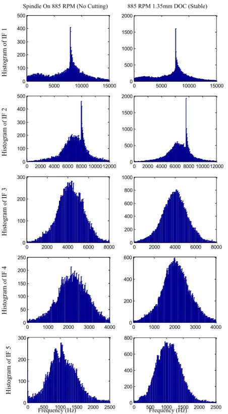
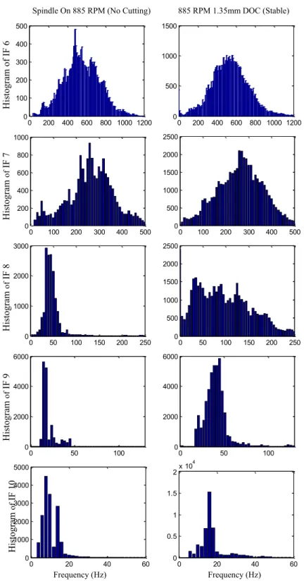
4.4 Histogram plots of individual IFs 1-5 at 885 rpm – workpiece ... 48

4.6 Top ten frequency modes for 1239 rpm dry-run workpiece vibrations ... 51

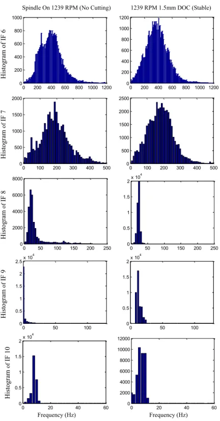
4.7 Top ten frequency modes for 1239 rpm and 1.5mm DOC chatter-free cutting ... 52

(12)

FIGURE Page 4.11 Top ten frequency modes for 885 rpm and 1.35mm DOC tool vibrations 57 4.12 Histogram plots of individual IFs 1-5 at 885 rpm – tool ... 58 4.13 Histogram plots of individual IFs 6-10 at 885 rpm – tool ... 59 4.14 Top ten frequency modes for 1239 rpm dry-run tool vibrations ... 61 4.15 Top ten frequency modes for 1239 rpm and 2 mm DOC tool vibrations .. 62 4.16 Histogram plots of individual IFs 1-5 at 1239 rpm – tool ... 63 4.17 Histogram plots of individual IFs 6-10 at 1239 rpm – tool ... 64 4.18 Comparison of chatter-free (left) vs. chatter (right) cutting for

workpiece at 885 rpm ... 68 4.19 Histogram plots of important modes for chatter-free (left) and

chatter (right) workpiece vibrations at 885 rpm ... 69 4.20 Phase plot and Poincare section of chatter-free (left) vs. chatter (right)

cutting for the workpiece at 885 rpm (top) and 1239 rpm (bottom) ... 70 4.21 Comparison of chatter-free (left) vs. chatter (right) cutting for

workpiece at 1239 rpm ... 72 4.22 Histogram plots of important modes for chatter-free (left) and

chatter (right) workpiece vibrations at 1239 rpm ... 73 4.23 Phase plot and Poincare section of chatter-free (left) vs. chatter (right)

cutting for the tool at 885 rpm ... 75 4.24 Comparison of chatter-free vs. chatter cutting for tool at 885 rpm ... 76 4.25 Histogram plots of important modes for chatter-free (left) and

chatter (right) tool vibrations at 885 rpm ... 77 4.26 Zoomed-in plots of individual IFs for chatter cutting workpiece

vibrations at 885 rpm which show the development of chatter; Modes as noted in Table 4.1: (A) IF 4; (B) IF 5;

(13)

FIGURE Page 4.27 Zoomed plots of the individual IFs for chatter cutting tool vibrations

at 885 rpm which show the development of chatter;

Modes as noted in Table 4.1: (A) IF 5; (B) IF 6; (C) IF 8, IF9 & IF10 ... 81 5.1 Comparison of numerical (left) and experimental (right) tool

vibration signals for chatter-free cutting ... 85 5.2 Comparison of numerical (left) and experimental (right) workpiece

vibration signals for chatter-free cutting ... 88 5.3 Comparison of numerical (left) and experimental (right) tool

vibrations for chatter cutting ... 91 5.4 Comparison of numerical (left) and experimental (right) workpiece

vibrations for chatter cutting ... 92 5.5 Comparison of tool (left) and workpiece (right) numerical chatter

vibrations for the onset of chatter (top) and further developed

chatter (bottom) ... 94 5.6 Comparison of tool (left) and workpiece (right) numerical chatter-free

vibrations ... 95 5.7 Stability diagram for depth-of-cut vs. spindle speed with a constant

feed rate of 0.09mm/rev ... 97 5.8 Workpiece response at 1800 rpm and 2.0mm (top), 2.1mm (middle),

and 2.2mm (bottom) DOCs ... 99 5.9 Tool response at 1800 rpm and 2.0mm (top), 2.1mm (middle),

and 2.2mm (bottom) DOCs ... 100 5.10 Workpiece response at 2250 rpm and 2.85mm (top), 2.95mm (middle),

and 3.0mm (bottom) DOCs ... 102 5.11 Tool response at 2250 rpm and 2.85mm (top), 2.95mm (middle),

and 3.0mm (bottom) DOCs ... 103 5.12 Workpiece response at 3500 rpm and 1.5mm (top), 3.05mm (middle),

(14)

FIGURE Page 5.13 Tool response at 3500 rpm and 1.5mm (top), 3.05mm (middle),

and 3.35mm (bottom) DOCs ... 106

6.1 Effective rake angle shown to be highly negative when chip thickness becomes small ... 110

6.2 Vibrating tooth path of the tool shown at different moments in time ... 112

6.3 Small element on the cutting tooth face of the micro-tool ... 114

6.4 The 2D lumped mass-spring-damper model of the micro-tool ... 115

6.5 Top view of the tool that shows the two bottom axial elements and the angle between them ... 116

7.1 Simulated force signal for pearlite material parameters at 75,000 rpm and 2μm/tooth feedrate ... 120

7.2 Simulated vibration signal for pearlite material parameters at 75,000 rpm and 2μm/tooth feedrate ... 121

7.3 Force simulation results for the conditions in [43] at 60,000 rpm and 9μm/tooth feedrate ... 123

7.4 Simulation vibration results for the conditions in [43] at 60,000 rpm and 9μm/tooth feedrate ... 124

8.1 X-direction force RMS values for varying helical angle ... 128

8.2 Y-direction force RMS values for varying helical angle ... 129

8.3 X- and Y-direction motion and motion IF plots for 60,000 rpm (left) and 75,000 rpm (right) spindle speed for a 45° helical angle ... 131

8.4 X- and Y-direction forces and force IF plots for 60,000 rpm (left) and 75,000 rpm (right) spindle speed for a 45° helical angle ... 132

8.5 X- and Y-direction motion and motion IF plots for 100,000 rpm spindle speed and 45° (left) and 40° (right) helical angles ... 134

(15)

FIGURE Page 8.6 X- and Y-direction forces and force IF plots for 100,000 rpm spindle

speed and 45° (left) and 40° (right) helical angles ... 135 8.7 X- and Y-direction motion and motion IF plots for 150,000 rpm spindle

speed and 45° (left) and 40° (right) helical angles ... 137 8.8 X- and Y-direction forces and force IF plots for 150,000 rpm spindle

speed and 45° (left) and 40° (right) helical angles ... 138 8.9 X-direction force RMS values for varying rake angle ... 139 8.10 Y-direction force RMS values for varying rake angle ... 140 8.11 X- and Y-direction motion and motion IF plots for 100,000 rpm (left)

and 75,000 rpm (right) spindle speeds for a 10° rake angle ... 142 8.12 X- and Y-direction forces and force IF plots for 100,000 rpm (left) and

75, 000 rpm (right) spindle speeds for a 10° rake angle ... 143 8.13 X (left) and Y (right) direction motion (top) and force (bottom) plots

for 150,000 rpm spindle speed and a 10° rake angle ... 144 8.14 X-direction force RMS values for varying system stiffness ... 145 8.15 Y-direction force RMS values for varying system stiffness ... 146 8.16 X- and Y-direction motion and motion IF plots for 75,000 rpm spindle

speed and natural frequencies of 4,035 Hz (left) and 6,000 Hz (right) ... 148 8.17 X- and Y-direction forces and force IF plots for 75,000 rpm spindle

speed and natural frequencies of 4,035 Hz (left) and 6,000 Hz (right) ... 149 8.18 X- and Y-direction motion and motion IF plots for 100,000 rpm spindle

speed and natural frequencies of 4,035 Hz (left) and 6,000 Hz (right) ... 152 8.19 X- and Y-direction forces and force IF plots for 100,000 rpm spindle

speed and natural frequencies of 4,035 Hz (left) and 6,000 Hz (right) ... 153 8.20 X- and Y-direction motion and motion IF plots for 150,000 rpm spindle

(16)

FIGURE Page 8.21 X- and Y-direction forces and force IF plots for 150,000 rpm spindle

speed and natural frequencies of 4,035 Hz (left) and 6,000 Hz (right) ... 155 A.1 LabView VI constructed for data collection ... 176 A.2 Proper configuration of the DAQ Assistant block by setting the

(17)

LIST OF TABLES

TABLE Page 3.1 Cutting Tests Performed and Operator Observations ... 36 4.1 Important Vibration Modes for the Workpiece and Tool ... 65 5.1 Tool Experimental and Numerical Chatter-Free and Chatter Modes... 84 5.2 Workpiece Experimental and Numerical Chatter-Free and

(18)

1. INTRODUCTION

1.1Turning Overview and Literature Review

Metal cutting technologies are important manufacturing processes for the production of quality products from a wide range of materials. Metal cutting consists of removing material from the workpiece with a cutting tool in order to sculpt a desired design. The inputs for the cutting process are the cutting tool design and constituent, workpiece configuration and material, cutting fluid, spindle speed, feed rate, depth-of-cut (DOC), and machine tool assembly [1]. The configuration of these parameters will have a major impact on the dynamics of the system which affects the overall vibrations. System vibrations have a direct impact on the tool wear, workpiece tolerance, surface roughness, and cutting forces which are main outputs for measuring cutting performance [1]. The advancement of technology and the need to improve efficiency requires improved tolerances and the use of higher cutting speeds. Higher cutting speeds increase the forcing frequency of the process greatly affecting the dynamic response. Enhanced knowledge of cutting dynamics will directly benefit the improvement of metal cutting. The turning process consists of a rotating workpiece secured by the chuck and tailstock, and a tool with only translational motion removing material to produce parts with a circular cross-section (Fig. 1.1). The amount of material removed during the

____________

(19)

turning process is determined through the selection of the chip thickness (feedrate) and DOC as illustrated in Fig. 1.2. The cutting tool inclination, rake, and lead angles are dominant tool parameters which affect the distribution of the cutting forces in the global coordinates at the cutting edge (Fig. 1.3).

Fig. 1.1 Basic lathe cutting configuration

(20)

Fig. 1.3 Illustration of main lathe cutting tool angles

Excessive machining vibrations such as chatter are detrimental to tool integrity and product quality, thus considered a main culprit in compromising manufacturing efficiency. Chatter is observed by the operator as excessive noise and poor workpiece surface finish and was investigated in the 1940s for its adverse effect on chip formation, surface roughness, and tool vibrations [2]. One mechanism which causes chatter is the regenerative effect. The regenerative chatter is due to the relative motion between the tool and workpiece as well as the phase difference between the current tool position and the tool position the previous revolution in time. As the tool and workpiece vibrate, a wavy finish is left on the surface of the workpiece, and when these motions become out of phase the instantaneous chip width will become increasingly large causing the vibration magnitude to continuously grow to an unstable limit. Mathematical modeling of the metal cutting process is effective for studying machining instability. General chatter vibrations of the machine tool were studied in [3] and the theory of nonlinear regenerative chatter was analyzed in [4] in which nonlinear stiffness was applied to the structure and a nonlinear force coefficient was used. In [5] nonlinearity was introduced

(21)

by the tool leaving the cut under excessive vibration amplitudes and through nonlinear force characteristics. These studies investigated the effect that nonlinearities have on traditional stability lobes resulting in stable, conditionally stable, and unstable regions. Analytical studies of 2 degree-of-freedom (DOF) cutting systems were analyzed in [6-8] to further investigate the effect of wave generation on instability and how frictional force affects the stability lobes. In [9] a milling stability diagram is developed by first linearizing a 2 DOF milling model, followed by selecting a chatter frequency, solving the eigenvalue, calculating the critical DOC, and determining the spindle speed. These early analytical models are expanded to a multidimensional model that includes tool nose radius [10, 11], process damping [12], and tool wear [13]. While analytical methods are effective at producing stability lobes, linearization necessarily obscures the true nonlinear characteristics, thus rendering the use of stability lobes for chatter suppression both inaccurate and ineffective. Also, the stability lobes are developed without regard to resulting vibrations [14], so stable cutting conditions that may have unacceptable vibration amplitude are not accounted for. Chatter therefore remains a major issue in today’s machine shops [15].

The methods reviewed provide limited insight into the nonlinear underlying dynamics of chatter vibrations because they do not allow for nonlinearities. To fully understand machining instability, nonlinear characteristics must be retained as machining is by nature nonlinear and non-stationary [16]. The advancement of computing power and nonlinear dynamic analysis techniques allows for further analysis of the machining process through the simulation of advanced models. Reference [17]

(22)

investigated the dynamics involved in the cutting process by analyzing a 3D model that includes friction and uses the systems boundary theorem to study the interactions between the tool jumping out-of-the-cut, tool rubbing but not cutting, and the tool cutting phases. In [16] phase portraits were used to provide insight into the state of the system but they failed to reveal detail information about the dynamics, and [18] analyzed the classic 1 DOF delay-differential equation with the previous workpiece motion assumed to be sinusoidal. Along with the study reported in [19] where subcritical Hopf bifurcation emerged in a 2 DOF nonlinear model, these studies concluded that bifurcated and possibly chaotic motion could be present in machining. It is suggested in [20] and [21] that 1 DOF models cannot resolve the complex nonlinear motions and thus models with more degrees of freedom are needed and should be judged on their ability to resolve nonlinear dynamics. The model in [22] used Simulink to configure different blocks together to incorporate nonlinear effects and predict surface generation. In [23] a comprehensive three-dimensional force model considering the tool nose radius and different tool angles was developed. However, these three-dimensional (3D) models fail to incorporate workpiece motion limiting the ability to fully investigate the dynamics. Turning is inherently a 3D process that includes the tool and workpiece vibrations which are necessarily coupled [24-25] due to nonlinear characteristics such as the tool jumping out of the cut and workpiece motions exceeding that of the tool [26]. Thus, to successfully model the turning process, the tool and workpiece motions have to be simultaneously considered. Of the handful of models that incorporate workpiece motions and dimensional force equations, only the comprehensive

(23)

three-dimensional model presented in [24-25] considers the simultaneous, coupled tool and workpiece vibrations without employing linearization techniques.

The analytical and numerical analysis of mathematical models is important for studying the cutting process and providing guidance for experimental research which would aid in achieving improved solutions for avoiding harmful vibrations. Analytical models develop stability lobes which benefit the machine operators by providing a guideline for chatter-free cutting parameters. However, to fully resolve the issue of chatter, the underlying dynamics must be fully understood. This can only be realized through complete nonlinear modeling and analysis of the coupled tool and workpiece interactions. Thus, it is important to investigate the ability of a mathematical model to capture the underlying dynamics so that the model can be confidently used to study the process. The thesis research presented will study the ability of the model in [24] to effectively capture the underlying dynamics of the turning process. In Section 3 the model will be briefly introduced and the experimental design used to capture tool and workpiece vibrations for model validation will be presented.

Adequate modeling or experimental analysis would not provide the desired insight if the analysis techniques used are not effective at handling nonlinear systems. Traditionally chatter is defined as the appearance of a chatter frequency close to a dominant frequency of the machine tool system, increasing vibration amplitude, poor surface finish, and increased noise [15]. The visual inspection of workpiece surface finish and the audible recognition of chatter by the operator are subjective methods for defining and identifying chatter, and resulted in delayed chatter detection in [26]. Thus,

(24)

it is important to monitor the system with a tool capable of quantitatively identifying and defining cutting instability. Analyzing the system in the frequency domain has been found to be effective for quantitative chatter recognition, and the analysis of numerical and experimental data overwhelmingly utilizes Fast Fourier Transform (FFT) for spectral analysis [11-13, 23]. Although commonly used, FFT has serious drawbacks in the processing of nonlinear and non-stationary signals because it is the integration of the signal over all time which is an averaging of the frequency spectrum with a fixed resolution [27]. Local properties and nonlinear interactions can be averaged out making FFT poor in resolving nonlinear features. In [28] the instability of a milling process is analyzed using discrete wavelet transform and the concept of energy variation. It is illustrated that instability, depending on the state of deterioration, could be multi-periodic, amulti-periodic, or chaotic. This demonstrates the need for analyzing machining in the time-frequency domain since dynamic instability is characterized by a change in the period and frequency that are coupled. Of the many time-frequency analysis tools available, instantaneous frequencies (IFs) determined by the Hilbert-Huang Transform (HHT) provides the best resolution needed in resolving the transition from stability to instability [29, 30]. The HHT applies a sifting process called Empirical Model Decomposition (EMD) to decompose a multi-component signal into a set of mono-component units called Intrinsic Mode Functions (IMFs). Once IMFs are obtained, Hilbert Transform is then performed to determine the IFs of the signal. Both IF and EMD have been successfully applied to the detection of damaged gears [31], the showing of different responses of a nonlinear rotor model [32], and the resolving of the

(25)

transition from stability to instability in a machining research [33]. Application of IF to experimental machining vibrations, however, is not available in the literature. Thus, in this research IF will be the main tool used to characterize the machining vibrations and FFT, phase portrait, and Poincare section will be applied to further validate the dynamic state of motion identified with IF. In Section 2 these analysis tools will be introduced and applied to example signals, and in Section 4 a method is developed and employed to effectively characterize experimental turning dynamics using IF. This will be followed by Section 5 where the model in [24] is validated and instability is investigated.

1.2 Micro-milling Overview and Literature Review

Micro-technologies are widely used in the area of medicine, life sciences, communications, and mobility [34], and as micro-technologies continue to be developed they will need increased functionality and to withstand harsher environments. This requires a wide range of materials and complex 3D features which increases the importance of micro-manufacturing research to meet and enhance these demands. Defined as cutting at values less than 1 mm [35], micro-milling is able to produce complex 3D miniature components out of a wide range of materials. Micro-milling is subject to sudden and excessive vibrations and forces that negatively impact the longevity of the tool and the ability to control component quality [36]. To address these challenges, modeling is important for gaining a better understanding of the effect different mechanisms and cutting parameters have on the dynamics. Also, modeling provides guidance for empirical research that assists in further understanding the process [35-36]. Modeling of the macro-milling process has been widely researched with many

(26)

analytical and time domain simulation methods developed. The analytical milling model in [9] that takes the Fourier series expansion of time-varying milling force coefficients is expanded to develop a three-dimensional chatter stability model for ball end, bull nose, and inclined cutting edges in [37]. The solution for these dynamic models is purely analytical and in the frequency domain, and requires the selection of a chatter frequency which is commonly chosen around a dominant mode of the system. A semi-discrete time domain solution is proposed in [38] that considers time-varying coefficients and is compared to the frequency domain solution which shows the two methods produce similar stability lobes. The analytical method is compared to a time domain technique which uses constant cutting force coefficients in [39] and it is shown that instability at higher speeds which is observed experimentally is not predicted. An improved three-dimensional cutting force model that accounts for tool helical angle is presented in [40] along with a new method for estimating the cutting force coefficients and run-out parameters. Cutting force coefficient models accurately predict the magnitude of forces but fail to resolve the higher frequency components seen experimentally unless the chip thickness is correctly developed and the constantly changing tool angles are accounted for. The model in [41] utilizes a nonlinear cutting force coefficient relationship to accurately predict the cutting forces as well as produce a nonlinear milling model.

Micro-milling is a highly nonlinear process so a time domain simulation method is preferred for studying the dynamics of the system since it allows for nonlinear characteristics and changing variables to be accounted for [14]. Micro-milling cannot directly adopt the methods used for modeling macro-milling due to different cutting

(27)

force mechanisms at work and the increased tool radius-to-feed rate ratio. Tool run-out affects the micro-milling process more due to the small size of the tool. Tool run-out was investigated experimentally in [42] using a laser displacement sensor, its effect on micro-milling was discussed in [35, 36], and simulated in [43] which demonstrated how run-out increases the cutting forces on the tool. Tool run-out is due to spindle-tool misalignment and imperfections in the micro-tool. These parameters are controlled through increasing the precision of the micro-cutting center and the uniformity of the micro-tool. The focus of this research is to investigate the effect that cutting parameters have on the instability of micro-milling and to ultimately determine the parameters critical to the process, so tool run-out is neglected in the model development. Another difference between macro and micro-milling is that as the tool approaches the workpiece, the material is compressed and is either plowed under or formed into a chip [44], and the minimum chip thickness determines whether a chip is formed. When the uncut chip thickness is less than the minimum chip thickness, all of the material is plowed under the tool and results in only plowing forces being present and the plowed material elastically recovering by some amount. To simulate the dynamics of the system, all of these nonlinear mechanisms acting on the micro-milling process need to be addressed.

An analytical model is developed in [45] that uses experimentally determined coefficients which help to accurately predict the magnitude of the forces and to quickly monitor cutting forces. A mechanistic force model that utilizes material properties as well as an experimental constant to calibrate the forces is developed in [46]. The model

(28)

in [43] utilizes cutting force coefficients and studies the effect that run-out and elastic recovery of the workpiece has on the cutting forces, however, this model does not always predict the high frequency components seen experimentally. Due to the micro-nature of the cutting process, the cutting forces are affected by the microstructure of the materials. A model was developed in [47, 48] that can handle multiple phases in the workpiece, and the cutting parameters for ferrite and pearlite are studied in depth. The force mechanism in [49] is based off of experimentally observed material flow angles and the chip formation is modeled as a process of shear where the shear zone is determined by the coefficient of friction between the chip and tool. This paper developed equations for contact friction, contact stress, and material spring back but was validated for low speeds only. The method in [50] developed cutting force coefficients that are independent of cutting process parameters and incorporates an effective rake angle. Here equations were developed for the cutting force coefficients and experimental data was used to determine these coefficients which proved effective in predicting the cutting forces under multiple cutting parameters. Another proven effective method for developing the cutting forces is the slip-line method. A very detailed and elaborate slip-line model is developed in [51] that accounts for many of the features that occur near the tool edge during cutting. Earlier slip-line models were developed in [52, 53] to predict the shearing and plowing forces. The slip-line model developed in [54] built upon and improved the model in [53] by accounting for the dead metal cap and the frictional forces associated with it.

(29)

The research in [43, 45-53] focuses on the development of a forcing mechanism that accurately simulates the forces in micro-milling. Validation is performed by comparing a few rotations of the cutter under stable cutting conditions with experimental data. Further analysis into the effect of process variables on dynamic stability is limited. Thus, little research has been done investigating the dynamics of micro-milling with the goal of better understanding how the cutting parameters including feed rate, DOC, and spindle speed, among others affect the stability of the system. This is important in determining the cutting parameters critical to the process. This research will investigate micro-milling through the development of a nonlinear dynamic model in Section 6 capable of resolving the nonlinear dynamic signature of the micro-milling process. The force mechanism will account for shearing and plowing forces, and the dynamic effective rake angle. A novel approach for determining the chip thickness by considering the elastic recovery of the material and the tool disengaging the workpiece is developed, and the tool helical angle is accounted for by assuming that the tool can be split into axial elements. This model is then validated in Section 7 by comparing the simulations with experimental data in literature as well as investigating the stability of these simulations using IF and FFT. Finally, the model is used to study the effect that the tool angles and system stiffness have on the resulting cutting forces and dynamic response in Section 8.

(30)

1.3 Research Objectives

The dynamic response of the tool in turning and micro-milling greatly affects the tool wear rate and cutting forces which increase the probability of tool failure. Excessive vibrations also impact workpiece tolerance and surface roughness which contributes to decreased process efficiency and is still a prominent issue in machining. This hinders the advancement of high speed machining because process nonlinearities are more prominent at high spindle speeds due to the increased forcing frequency. To fully address the issue of excessive machining vibrations, the underlying dynamics of the process need to be fully understood. Comprehensive mathematical models provide an effective means for studying the process and obtaining an enhanced understanding of the underlying dynamics as well as developing solutions and control algorithms for handling instability. However, mathematical models must be experimentally validated in order to be established as a competent tool for dynamic analysis. In addition, appropriate nonlinear analysis techniques need to be applied in order to unveil the true dynamics of the system. Thus, the overall objective of the research is to provide further insight into the underlying dynamics of the machining process through the analysis and experimental validation of the turning model in [24] using IF, and the analysis of micro-milling dynamics by developing a nonlinear dynamic model. The research objectives will be accomplished through the following tasks:

 Develop an experimental test set-up to acquire tool and workpiece vibrations  Generate a procedure for analyzing experimental vibrations using IF

(31)

 Compare experimental and numerical dynamics using the model in [24]

 Use the model in [24] to produce a thorough stability diagram considering the dynamics of both the tool and workpiece

 Confirm tool – workpiece interaction is prominent and non-negligible  Investigate high speed turning dynamics using the model in [24]

 Develop a nonlinear micro-milling model which correctly calculates the instantaneous chip thickness, accounts for tool geometry, workpiece properties, and nonlinear forcing mechanisms

 Compare model simulations to experimental data in literature

 Investigate the effect that process parameters have on the resulting cutting forces and dynamic stability

The realization of the tasks presented will provide further insight into machining instability as well as provide tools and knowledge needed to accurately characterize the dynamics of machine cutting technologies and develop solutions to mitigate excessive vibrations.

(32)

2. INTRODUCTION AND FUNDAMENTALS OF ANALYSIS TOOLS

2.1Fundamentals of Fourier Transform

The analysis method developed by John Fourier has been used in all areas of engineering and is a common method for converting an analog signal, , into frequency-domain information [55, 56]. This analysis is commonly termed as the Fourier transform and is used to reveal the spectral characteristics of a signal. Engineers usually associate the Fourier transform as an extension of the Fourier series by allowing the period, T, of the signal to approach infinity. Fourier series is used in vibrations to develop an analytical representation in time of a periodic time signal [55]. Hence, it is an orthogonal projection of the signal with respect to the basis set which are typically the sine and cosine functions. The Fourier series of the time function, , is commonly expressed in vibrations courses using the following equations [55],

(2.1) where: (2.2) (2.3) (2.4) (2.5)

(33)

To extend the Fourier series to Fourier transform, the period T is extended to infinity and the Fourier series is expressed as:

_(2.6)

The integral inside the brackets is the Fourier transform and for a finite energy function of real-variable, t, the Fourier transform is expressed as:

_(2.7)

The computation of Fourier series and Fourier transform requires integration and analytically describes the signal through elementary functions such as sine and cosine. The signals encountered in real life are usually not represented by these elementary functions, so to apply these techniques to real-world signals, the discrete Fourier series and discrete Fourier transform are directly computed using numerical algorithms, thus producing an approximate spectrum of the original analog signal. The Fourier transform integral in (2.7) can be approximated using the following discrete form,

(2.8)

This series sum can be applied to discretely sampled data where ∆t is the sampling rate. The Fourier transform is incorporated in the analysis conducted throughout this research due to its extensive use in industry and research for spectral analysis of vibration signals. This will allow for a comparison to the effectiveness of IF and to confirm observations made in the time-frequency domain.

(34)

2.2 Fundamentals of Instantaneous Frequency

Machining is a nonlinear and non-stationary system which can have a time-varying amplitude and frequency. The commonly used FFT analysis is not able to resolve time-varying frequencies in the signal and the objective of the research to observe the transition of system dynamics requires the ability to resolve individual spectral components in time. Instantaneous Frequency (IF) as presented in [30] is briefly reviewed in the followings. The idea of instantaneous frequency is different from the traditional definition of Fourier frequency which requires a complete revolution of a sine or cosine wave. Also, IF encountered an early difficulty due to the non-unique way of defining the instantaneous frequency [30]. A general signal with both time-varying amplitude and frequency can be written as:

(2.9)

where is the instantaneous amplitude and is the instantaneous phase. There are an infinite number of ways to express a signal in the form shown in Eq. (2.9) and hence the difficulty of not having a unique definition of instantaneous frequency [32]. This was overcome by using the Hilbert Transform, defined in Eq. (2.10) to make the data analytical.

(2.10) where P is the Cauchy principle value. From Eq. (2.10), and form the complex pair for the analytical signal, .

(35)

This provides a uniquely defined instantaneous amplitude and instantaneous phase which are expressed as:

(2.12)

(2.13)

Then the instantaneous frequency is defined as the time derivative of the instantaneous phase and is provided in Eq. (2.14) where it is also converted to hertz.

Hz (2.14)

This definition for instantaneous frequency works well for mono-frequency signals but does not work well for multi-component signals [30, 32]. This prompted the development of a process that decomposed the original signal into its multiple mono-frequency components so that the definition of IF above could be applied to each individual component. The Empirical Mode Decomposition (EMD) method is described in [30]. This method is based on the assumption that the original signal is composed of several intrinsic mode functions (IMFs). An IMF is defined as a function with the two following characteristics: (1) the number of extrema, zeros, and zero crossings must either equal or differ at most by one and (2) at any point in time the mean value of the envelope defined by the local maxima and the envelope defined by the local minima equals zero. The EMD process is adaptive with the basis of the decomposition based on the data itself making it suitable for resolving data that are both nonlinear and non-stationary. The basis of the method is to decompose the signal based off of the characteristics of the IMFs in the data empirically. The EMD process can be implemented using the following procedure:

(36)

1. Identify the extrema and then connect the local maxima with a cubic spline to make the upper envelope and connect the local minima with a cubic spline to make the lower envelope.

2. Subtract the mathematical mean of the two envelops from the original signal to obtain the first component, h1.

3. Continue the sifting process given in Eq. (2.15) until the first IMF of the signal is obtained. The stop criterion in [30] is used to determine when adequate sifting has been done and an IMF has been identified.

4. Once this is done, the first IMF is obtained. This would be the mode with the highest frequency and is denoted as c1 in Eq. (2.16). Next the first IMF is

extracted from the original data has shown in Eq. (2.17).

(2.15)

(2.16)

(2.17)

5. The residue, r1, still containing information of the lower frequency modes is then

treated as new data, and the sifting process is performed on it.

6. This procedure is repeated until all of the IMFs of the system have been identified and extracted from the original signal leaving only the final residue which is a monotonic function in which no other IMFs can be extracted.

The original signal can be restored by simply summing all the IMFs and the residue as shown in Eq. (2.18).

(37)

Once all of the IMFs have been extracted from the original signal, a complete set of mono-component signals which make up the original signal are obtained. The Hilbert transform is then applied to each IMF to determine the instantaneous frequency.

2.3 Introduction to Phase Portrait and Poincare Section

Phase portraits and Poincare sections are useful tools for classifying the state of motion of a nonlinear system [57]. The state space in nonlinear dynamics as defined in [58] is a generalization of the traditional phase space of the Hamiltonian dynamics. The phase diagrams contain important information about the behavior of a nonlinear dynamic system. By plotting the displacement vs. velocity of a system, a qualitative description of the state of motion of the system is obtained. The phase diagram of a linear system will typically have one loop indicating that the phase space and thus the dynamics of the system repeat in time, suggesting a state of periodic motion. A nonlinear system may have changing dynamics in time and thus the phase diagram will demonstrate this change of dynamics. Information about the attractors of the system such as a single point, limit cycle, and torus can be obtained using phase diagrams [58]. A Poincare section can be obtained by sampling the phase diagram at a particular frequency. If a data point of the displacement and velocity response of a perfect sine wave is pulled out once every period, then this will result in a single point in the velocity vs. displacement plane because history will repeat itself. If there are two modes in the signal composed of two perfect sine waves, then there will be two points in the Poincare section. For a chaotic response when history doesn’t repeat itself there will be an infinite number of points in the Poincare section. Thus, the phase and Poincare plots can be used to obtain

(38)

a qualitative overview of the dynamics of a nonlinear system, but are not able to provide detailed information about the frequencies of the system.

2.4 Summary and Examples

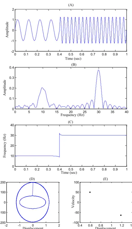
This subsection will utilize various signals to visualize differences in the ability of the analysis tools described to investigate the dynamics of a frequency- and amplitude-modulated signal. As described in Section 2.1, Fourier transform is a linear transformation which attempts to describe the signal as the elementary functions sine and cosine. The Fourier transform is also globally inclusive as it integrates the signal over the full length of time and thus cannot identify local properties of the signal. Signals in the real-world are usually not represented by these elementary functions and have time-varying frequency characteristics. Instantaneous Frequency utilizes the signal itself to decompose it into its mono-frequency components and doesn’t try to describe the signal as elementary functions as this is unrealistic for nonlinear and real-world signals. In addition, IF identifies the exact frequency values at that moment in time so it provides the best time frequency resolution possible. Figure 2.1 is the analysis of a basic low frequency signal with a higher frequency wave riding on it. The discrete Fourier transform (DFT) plot shows that the higher frequency component of 55 Hz, which is lower in energy, is not as dominant as the 10 Hz component. The IF plot clearly shows both the 55 and 10 Hz modes throughout the duration of the signal. The phase portrait reveals a stable system which is repeating its motion in time and the Poincare section contains two points indicating there are two frequencies in the signal. Figure 2.2 is a signal with a time-varying frequency and amplitude. At the 4 second mark, the

(39)

frequency of the signal changes from 10 to 30 Hz and the amplitude increases from 1 to 1.25. The DFT plot is unable to provide any information about the changing frequency spectrum and shows both modes as if they were in the signal throughout all time. The IF plot captures the change of frequency in the signal right at the 4 second mark and decidedly identifies both frequencies. This demonstrates the ability of IF to locate the time moment when the dynamics of the signal changed. The phase portrait clearly shows that two frequencies are present and the Poincare section has two points corresponding to the two frequencies of the signal. The previous two examples illustrated the accuracy of IF to identify the frequency components in the signal and the advantage that IF provides when analyzing a frequency-modulated signal. The following example demonstrates a case when Fourier transform is not able to provide any useful information, but IF is able to show the exact frequency spectrum of the signal. Figure 2.3 is a signal where the amplitude and frequency are linearly modulated in time. The Fourier transform suggests that there are a wide range of frequencies throughout the signal. The IF plot correctly shows a linearly changing frequency spectrum. The phase diagram has a spiral due to the linearly increasing frequency and the Poincare section has multiple points which are not repeating in time because the dynamics are changing from one moment in time to the next.

(40)

Fig. 2.1 Time response (A), DFT (B), IF (C), Phase portrait (D), and Poincare section (E) of the following signal.

0 0.1 0.2 0.3 0.4 0.5 0.6 0.7 0.8 0.9 1 -200 -100 0 100 200 0 10 20 30 40 50 60 70 0 20 40 60 0 0.1 0.2 0.3 0.4 0.5 0.6 0.7 0.8 0.9 1 0 20 40 60 80 100 -200 -100 0 100 200 -1 -0.5 0 0.5 1x 10 4 2 4 6 8 10 4000 6000 8000 10000 (A) Time (sec) Am plitu de (B) Frequency (Hz) Am plitu de Frequ en cy ( Hz) (C) Time (sec) (E) Displacement Velo city Displacement Velo city (D)

(41)

Fig. 2.2 Time response (A), DFT (B), IF (C), Phase portrait (D), and Poincare section (E) sampled at 10 Hz of a mono-frequency signal.

0 0.1 0.2 0.3 0.4 0.5 0.6 0.7 0.8 0.9 1 -2 -1 0 1 2 0 5 10 15 20 25 30 35 40 0 0.1 0.2 0.3 0.4 0 0.1 0.2 0.3 0.4 0.5 0.6 0.7 0.8 0.9 1 0 10 20 30 40 -2 -1 0 1 2 -200 -100 0 100 200 0.4 0.6 0.8 1 1.2 1.4 -100 -50 0 50 100 (B) Frequency (Hz) Am plitu de Frequ en cy ( Hz) (C) Time (sec) (E) Displacement Velo city Displacement Velo city (D) (A) Time (sec) Am plitu de

(42)

Fig. 2.3 Time response (A), DFT (B), IF (C), Phase portrait (D), and Poincare section (E) sampled at 10 Hz of the following chirp signal.

0 0.1 0.2 0.3 0.4 0.5 0.6 0.7 0.8 0.9 1 -1 -0.5 0 0.5 1 0 10 20 30 40 50 60 0 0.02 0.04 0.06 0.08 0 0.1 0.2 0.3 0.4 0.5 0.6 0.7 0.8 0.9 1 0 10 20 30 40 50 -1 -0.5 0 0.5 1 -400 -200 0 200 400 0 0.2 0.4 0.6 0.8 1 -50 0 50 100 150 200 (A) Time (sec) Am plitu de (B) Frequency (Hz) Am plitu de Frequ en cy ( Hz) (C) Time (sec) (E) Displacement Velo city Displacement Velo city (D)

(43)

The final example in this section is a signal which more accurately represents vibrations in the machining process. In machining there are typically at least two frequencies in the signal which are the tool natural frequency and the spindle speed. Figure 2.4 demonstrates a signal that has a higher frequency component in 200 Hz which would correspond to the tool natural frequency and a lower frequency component in 25 Hz which relates to the spindle speed. This signal also demonstrates period-doubling bifurcation of the higher frequency component at the 0.5 second mark. The DFT shows all three frequencies and the amplitude of each frequency corresponds to the amplitude of that component of the signal. The IF plot captures the moment in time that period-doubling bifurcation occurs as well as identifies the frequency value for each mode. As the signal shifts there are discontinuities that occur which result in sharp fluctuations seen in the IF plot until the signal settles out. The phase diagram demonstrates multiple circles and the Poincare section has only two points suggesting there are two frequencies in the signal because the Poincare sampling rate is a multiple of both higher frequencies. This example was performed to illustrate the ability of IF to accurately characterize the transition to instability of a nonlinear signal. The route-to-chaos of a dynamic system involves bifurcations of the signal which are identified in the frequency domain [28]. Fourier transform is not able to observe this transition and thus IF is the analysis tool of choice employed throughout this research to identify the state of motion of a system.

(44)

Fig. 2.4 Time response (A), DFT (B), IF (C), Phase portrait (D), and Poincare section (E) sampled at 25 Hz of the following signal that experiences a bifurcation. 0 0.1 0.2 0.3 0.4 0.5 0.6 0.7 0.8 0.9 1 -2 -1 0 1 2 0 50 100 150 200 250 0 0.1 0.2 0.3 0.4 0.5 0 0.1 0.2 0.3 0.4 0.5 0.6 0.7 0.8 0.9 1 0 100 200 300 400 500 -2 -1 0 1 2 -2000 -1000 0 1000 2000 0.54 0.56 0.58 0.6 0.62 0.64 950 1000 1050 1100 (A) Time (sec) Am plitu de (B) Frequency (Hz) Am plitu de Frequ en cy ( Hz) (C) Time (sec) (E) Displacement Velo city Displacement Velo city (D)

(45)

3. TURNING EXPERIMENT

3.1 Description of 3D Turning Model

The turning experiment is designed utilizing the observations made by the research in [24]. The basis of the model in [24] is that the workpiece consists of three distinct sections: un-machined, being machined, and machined. The un-machined section is fixed to the spindle with the machined section supported by the tailstock. The workpiece in Fig. 3.1 is modeled as three rotors connected to each other via a shaft of negligible mass. The rotors are assumed to be rigid and remain vertical at all times. Eccentricity is assumed to be proportional for each section, and static deflection of the workpiece is assumed for a uniform bar since the DOC is small compared to the overall diameter. The mass of each section is assumed to act on its own center of mass and the thickness of each rotor is kept the same as the length of that respected section. This makes the thickness of the being machined section, to, very small. However, this is

where the cutting force acts and thus the response of Rotor 2 is important to the dynamics of the 3-rotor system. The workpiece considers the changing stiffness and mass due to material continuously being removed during cutting. This makes the stiffness and mass of the workpiece nonlinear, and the tool is modeled with a linear and nonlinear stiffness term.

(46)

Fig. 3.1 Workpiece configuration (top) and workpiece modeled as 3 rotors (bottom)

The equations of motion for the model are given in Eqs. (3.1-3.3), where functions are nonlinear functions defined in [24] and the subscript 2 corresponds to Rotor 2.

(3.1) (3.2) (3.3)

The tool is only considered in the direction and workpiece motions in the Z-direction are assumed negligible. The force model used for the system is similar to the

(47)

3D force model developed in [23] except that the tool nose radius is not considered and a new method for calculating the instantaneous chip cross-sectional area and instantaneous DOC is developed. The base form for the force equations as a function of the normal, , and frictional, , forces are expressed in Eqs. (3.4-3.6) where is the chip flow angle, and coefficients are determined from the coordinate transformation matrices as

functions of lead, inclination, and rake angles.

(3.4)

(3.5)

(3.6)

As the DOC used is much larger than the tool nose radius, the effect of nose radius is considered negligible. Many models assume that either the chip thickness or DOC is constant; however, in reality the tool and workpiece vibrate simultaneously so the chip width changes due to the motion of the tool at the previous workpiece revolution and the DOC changes due to the instantaneous position of the workpiece and tool. In this model, the frictional and normal forces are assumed to be a function of the instantaneous chip thickness and DOC. In addition to the forces produced due to cutting, the workpiece has restoring forces which occur when the workpiece is deflected.

3.2 Experiment Design

The research in [24] demonstrates that the workpiece is critical to the underlying dynamics of the system and in [26] the detection of chatter is more prominent in the workpiece vibrations rather than the tool vibrations. However, tool vibration is predominantly the only variable investigated in research because it can easily be

(48)

obtained using contact sensors. Thus, in this research the objective is to investigate both the tool and workpiece vibrations. There are many different direct and indirect methods for monitoring the turning process as discussed in detail in [29]. Indirect measurements deal with measuring process variables such as motor current and then relating this to cutting force through mathematical and/or empirical relations. Direct methods allow for the direct measurement of the variable of interest which results in a high degree of accuracy. Tool vibrations can be directly measured using contact sensors such as force dynamometers, accelerometers, and strain gauges. However, contact sensors come with a mechanical resonance frequency that must be avoided. This limits the available sensing bandwidth and thus the ability to accurately capture high frequencies characteristic of a nonlinear process. Also, contact sensors are not applicable for measuring workpiece vibrations. Non-contact sensors such as eddy-current probes and displacement lasers can accurately capture vibration over a broad range of frequencies and are not limited by their mechanical resonance. Non-contact sensors also provide the advantage of ensuring the dynamics of the system is not altered since they are mounted independent of the process of interest. However, various non-contact sensors such as eddy-current probes require a very small measuring range which increases the probability of damaging the sensor during the event of tool failure or increased workpiece deflection. The availability of long range laser displacement sensors overcomes this difficulty.

The following experiment utilizes a laser displacement sensor which has a wide bandwidth and submicron resolution to capture both the tool and workpiece vibrations

(49)

during cutting. The tests were set up on a Victor lathe with 1,800 rpm capacity (Fig. 3.2). An NI6009 DAQ running at a sampling rate of 48 kHz was coupled with a Keyence LK-G 157 that was mounted above the workpiece on a rigid stand independent of the lathe and shielded from chips with an acrylic sheet (Fig. 3.3). For tool vibrations, the stand is adjusted so that the laser is mounted above the tool similar to the workpiece configuration. The laser controller was used to calibrate the system for the desired target material and to ensure no filtering of the data occurred. The DAQ was connected to a PC and a LabView program was built to continuously record and save the data. The details of the LabView program and the laser controller settings used are provided in Appendices A and B.

Fig. 3.2 Picture of experimental set-up

Stand Supporting Laser

Manual Lathe Cart with Data Acquisition

(50)

Fig. 3.3 (A) Schematic of laser set-up; (B) and (C) Experimental set-up of laser mounted above workpiece Laser Tool (A) (B) (C)

(51)

3.3 Experiments

A Kennametal SSDC 45° tool holder with a SCMT-LF insert having a side cutting edge angle of 45°, inclination angle of 5°, rake angle of 5°, and a nose radius of 0.8mm was used for the cutting tests. The cutting was performed without coolant and a new insert was used for each test to ensure that tool wear did not affect the system. The workpiece material was a 25.4mm in diameter 4140 steel bar configured to be as similar as possible to the workpiece considered in [24] without wasting material. Here the workpiece has a significant un-machined section as well as a significant machined section as seen in Fig. 3.4 (A). However, to efficiently use the workpiece material available, the workpiece was set up with stepped sections for the changing DOC tests as shown in Fig. 3.4 (B). The section being machined was pre-configured to achieve about 10mm of cutting at different DOCs for approximately 5 tests before the workpiece had to be re-configured. The un-machined section was approximately 150mm while the machined section varied from ~50mm to ~100mm. This also placed the cutting and laser measurement towards the center of the workpiece where the largest deflection is experienced. To study turning dynamics, changing DOC tests were performed for different spindle speeds with a constant feed. The lathe was run at various spindle speeds to eventually have 885 and 1239 rpm determined along with a constant feed of 0.09mm/rev as the smoothest speed of operation. To accurately record the DOC of each cut, the diameter of the workpiece was measured before and after each cut. The tests performed along with the observations made are tabulated in Table 3.1. Figure 3.5 gives

(52)

the observations noted by the operator as excessive noise and chatter associated with poor workpiece surface finish.

Fig 3.4 (A) Workpiece configuration for model in [24]; (B) Workpiece configuration for changing DOC tests used in experiment

(A)

(53)

Fig. 3.5 Graph of operator observed stability points

Table 3.1 Cutting Tests Performed and Operator Observations Machined

Diameter (mm) Diameter (mm) Unmachined Cut (mm) Depth of Observations 885 RPM Workpiece Vibrations 20.4 20.9 0.25 stable cutting 20.3 22.2 0.95 stable cutting 20.2 23.2 1.5 noise/poor surface 20.2 24.2 2 noise/poor surface 885 RPM Tool Vibrations 20.43 22.1 0.835 stable cutting 21.1 23.1 1 stable cutting 21.4 24.1 1.35 stable cutting 20.3 23.8 1.75 noise/poor surface 1239 RPM Workpiece Vibrations 19.94 20.83 0.445 stable cutting 19.94 21.94 1 stable cutting 20.1 23.1 1.5 stable cutting 20 23.6 1.8 stable cutting

20.2 25.2 2.5 light noise/poor surface

1239 RPM Tool Vibrations 20 24 2 stable cutting 20 24.8 2.4 stable cutting 0 0.5 1 1.5 2 2.5 3 800 1000 1200 1400 Depth -of -cu t (mm) Spindle Speed (rpm) Chatter Workpiece Stable Workpiece Chatter Tool Stable Tool

(54)

3.4 Amplitude Analysis of Raw Vibration Data

The raw vibration signals are analyzed to determine the change in amplitude for the response under different cutting conditions. Since it is difficult to accurately quantify the vibration magnitude just by observing the raw signal, the root-mean-square (RMS) method is used. The RMS is a measure of the magnitude of a set of values, so as the vibration magnitude increases, the RMS values increase as well. The RMS plots presented account for the offset of the original signal.

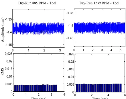
The dry-run vibrations with the spindle off are compared to the dry-run vibrations of the workpiece with the workpiece rotating at 885 rpm and 1239 rpm in Fig. 3.6. The vibrations at 885 rpm have maximum values around 40 microns and the 1239 rpm has maximum values around 50 microns. The RMS for 1239 rpm is twice as large as that at 885 rpm suggesting that the whirling at 1239 rpm is much larger than what is portrayed by the vibration signal. This is because at 885 rpm there are just a few points which stray up to 40 microns in the vibration signal giving the image that the difference between the 885 rpm and 1239 rpm whirling isn’t very large. However, the RMS provides insight about the overall magnitude of the entire set of values demonstrating that at 1239 rpm the vibration values consistently reach magnitudes much larger than the 885 rpm case. The dry-run vibrations for the tool at 885 rpm and 1239 rpm are shown in Fig. 3.7. The dry-run vibrations of the tool are slightly larger than the spindle not on vibrations in Fig. 3.6 and the 885 and 1239 rpm have similar vibration and RMS magnitudes. Thus, the lathe machine has similar vibration magnitudes at each speed but workpiece whirling is much larger at 1239 rpm.

(55)

Fig 3.6 Vibration response for dry-run spindle not on (left), dry-run at 885 rpm for the workpiece (middle), and dry-run at 1239 rpm for the workpiece (right)

Fig. 3.7 Vibration response for dry-run at 885 rpm for the tool (left) and dry-run at 1239 rpm for the tool (right)

0 1 2 3 4

-0.05 0 0.05

Dry Run Spindle Not On

Time (sec) A m p lit u d e ( m m ) 0 2 4 6 8 -0.05 0 0.05 Time (sec) A m p lit u d e ( m m )

Dry Run 885 RPM - Work-piece

0 2 4 6 -0.05 0 0.05 Time (sec) A m p lit u d e ( m m )

Dry Run 1239 RPM - Work-piece

0 1 2 3 4 0 0.005 0.01 0.015 0.02 0.025

Dry Run Spindle Not On

Time (sec) R M S 0 2 4 6 8 0 0.005 0.01 0.015 0.02 0.025

Dry Run 885 RPM - Workpiece

Time (sec) R M S 0 2 4 6 0 0.005 0.01 0.015 0.02 0.025

Dry Run 1239 RPM - Workpiece

Time (sec) R M S 0 1 2 3 -1.45 -1.4 -1.35

Dry Run 885 RPM - Tool

Time (sec) A m p lit u d e ( m m ) 0 1 2 3 4 5 -1.45 -1.4 -1.35

Time (sec) A m p lit u d e ( m m ) 0 1 2 3 4 0 0.005 0.01 0.015 0.02 0.025

Time (sec) R M S 0 2 4 6 0 0.005 0.01 0.015 0.02 0.025

Time (sec)

R

M

S

Time (sec) Time (sec) Time (sec)

Am plitu de ( m m ) RMS

Dry-Run Spindle Not On Dry-Run 885 RPM – Workpiece Dry-Run 1239 RPM – Workpiece

Time (sec) RMS Am plitu de ( m m )

Dry-Run 885 RPM - Tool Dry-Run 1239 RPM - Tool

(56)

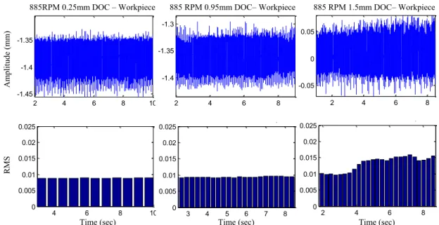
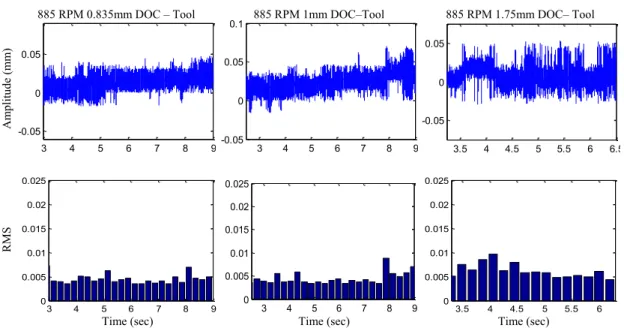
Chatter-free and chatter cutting workpiece vibrations at 885 rpm are compared in Fig. 3.8. The chatter-free vibrations at 0.25 and 0.95mm DOC have similar vibration magnitudes. The chatter cutting at 1.5mm DOC demonstrates a clear increase in vibration magnitude. The chatter-free vibrations for 1239 rpm at 0.445 and 1.5mm DOCs in Fig. 3.9 have different vibration magnitudes with the cutting at 1.5mm DOC having larger vibrations. The chatter cutting at 2.5mm DOC at 1239 rpm shows an increase in vibration magnitude. Here cutting did not last very long due to the intense chatter observed by the operator so enough time was not given for the vibration magnitude to continue to increase. The tool response in Fig. 3.10 shows similar vibrations for the chatter-free cases of 0.835mm and 1mm DOCs at 885 rpm. The chatter cutting at 1.75mm DOC and 885 rpm demonstrates an impulse in vibration magnitude at 4