Flexicurity and Job Reallocation

Flexicurity and Job Reallocation

Editor: Martina Flockerzi University of St. Gallen Department of Economics Varnbüelstrasse 19 CH-9000 St. Gallen Phone +41 71 224 23 25 Fax +41 71 224 31 35 Email [email protected] Publisher: Electronic Publication: Department of Economics University of St. Gallen Varnbüelstrasse 19 CH-9000 St. Gallen Phone +41 71 224 23 25 Fax +41 71 224 31 35 http://www.vwa.unisg.ch

Flexicurity and Job Reallocation

Author’s address: Prof. Christian Keuschnigg IFF-HSG Varnbüelstrasse 19 9000 St. Gallen Tel. +41 71 224 25 20 Fax +41 71 224 26 70 Email [email protected] Website www.iff.unisg.ch Thomas Davoine IFF-HSG Varnbüelstrasse 19 9000 St. Gallen Tel. +41 71 224 2156 Fax +41 71 224 2670 Email [email protected]

Abstract

This paper develops a general equilibrium model with safe and risky jobs where unemployment is concentrated in a highly productive but volatile sector. Frictional unemployment arises in the process of job creation, firing and retraining for alternative employment. The paper derives an optimal welfare policy which combines the design of the tax schedule with three pillars of the `flexicurity' model. The optimal policy is characterized by (i) a progressive wage tax schedule; (ii) a wage subsidy to re-employed workers; (iii) unemployment insurance benefits; (iv) job protection to contain firing; and (v) active labor market policy to facilitate labor reallocation.

JEL-Classification

J64, J65, J68, J32, H30.

Keywords

1

Introduction

For decades, high unemployment has plagued welfare states especially in Europe. The causes of unemployment are manyfold, and each one probably requires its own remedy. It is often argued that increasing globalization and the faster pace of technological progress lead to more volatile employment relationships, shorter job tenure and an increasing need for retraining of previously acquired skills (e.g. Brown, Merkl and Snower, 2009a, and Ljungqvist and Sargent, 1998). Part of unemployment thus results from an increasing speed of labor reallocation across different tasks with different skill requirements. Given the need to facilitate and speed up reallocation towards alternative employment, a suc-cessful policy might be the flexicurity model consisting of three pillars: insurance of the unemployed, active labor market policy (ALMP) to speed up transition into new jobs, and firing flexibility to close down unproductive jobs and replace them with new ones. Denmark’s success in reducing its unemployment rate from about 10% to 5% over the 1990’s is often attributed in good part to the flexicurity model.

The three pillars of flexicurity address separate channels of the labor market impact of welfare policies. Unemployment insurance (UI) is a central pillar of the welfare state and addresses a market failure due to missing private insurance markets for labor income risk. Developed countries spend up to 2% of GDP on UI (see OECD, 2009). Gruber (1997) estimated that the reduction in an unemployed workers’ consumption would be three times larger without UI (a 22.2% drop instead of 6.8%). Using a ‘sufficient statistics’ approach that avoids functional form assumptions, Chetty (2008) estimated that the current level of UI (replacement rate near 50%) is close to optimal in the US. There is consensus on the negative sign of the effect of UI on employment, but less so on its magnitude (see Holmlund, 1998). In their survey, Krueger and Meyer (2002) consider that a fair summary value for the effect of UI on employment is an elasticity of unemployment duration with respect to benefits of 0.5. There seems to be no or a positive impact of UI on wages or reservation wages.1

The most immediate effect of employment protection (EP), independent of whether it comes as an administrative cost or as a firing tax, is to reduce job separation and, thereby, contribute to lower unemployment. On the negative side, EP makes firms reluctant to hire workers in the first place if they find it difficult and costly to separate again when prospects become unfavorable. For this reason, high levels of EP have long been blamed for high European unemployment rates. The flexicurity model advises a low level of EP, at least lower than in many generous European welfare states, since it is argued that the positive effect of more hiring on the unemployment rate outweighs the negative effect of a higher separation rate.

This ambiguity is reflected in empirical research on how EP affects the labor market. Empirical studies consistently find that EP reduces flows into unemployment, but fail to report a reliable effect of EP on employment levels which points to a negative effect on hiring. The survey by Addison and Teixeira (2003) documents the heterogeneity of empirical findings since the original study by Lazear (1990). For instance, the summary table in Boeri and Jimeno (2005) shows only 5 significant coefficients out of 24. Heckman and Pages (2000) find significant positive effects of EP on unemployment. They estimate that the average 3 months of firing costs in Latin America amounts to a loss of 5.5% points of employment (for an average of 7.4% of unemployment). On the other end, OECD (1999) reports no significant effects of EP. Based on their empirical estimates, Belot, Boone and van Ours (2007) calculate an optimal level of employment protection which is positive and moderate: for instance, the growth maximizing level of protection for open-ended contracts is around 0.37 (on a scale from 0 to 1), corresponding to 1999 levels of protection in countries like Italy, Switzerland or the UK.

Active labor market policy (ALMP) mostly aims to support job search effort of un-employed workers, to develop their skills and make them more attractive to potential

3 reported by Petrongolo, 2008, and the study itself) arrive at different conclusions. They either find no statistically significant effect (in 6 cases) or statistically positive effects (higher UI benefits raise wages) which are often moderate or significant only for some subgroups (in the 4 other cases). Higher UI either raises wages or has no effect. The theoretical model below excludes wage effects.

employers, and to retrain for different jobs with alternative skill requirements. Total spending on labor market policies has grown to significant levels over the years. Accord-ing to OECD (2009), member countries spent on average 1.5 % of GDP in 2006 with some countries spending up to 3.4%. The fraction devoted to some form of active measures has grown from 35% in 1985 to 42% in 2007 (Martin and Grubb, 2001; and OECD, 2009). Several empirical studies show that monitoring and sanctions increase search efforts by unemployed workers more than the reduction in unemployment benefits (reported by Nunziata, 2008). Early empirical studies find negative or no significant effects of ALMP training programmes in the short-run (e.g. see the surveys Heckman, Lalonde and Smith, 1999; Martin and Grubb, 2001; Kluve, 2006), mostly due to a lock-in effect, but recent studies have data to focus on long-run effects. For instance, Lechner, Miquel and Wun-sch (2010) find that the re-employment probability increases by 20 to 40% and monthly earnings are higher by 0 to 550 Euro, depending on the training type.

There has been extensive theoretical research on different causes of unemployment and ways to reduce it. Economists have often studied the effects of different policies in isolation or in pairs. Using a combination of instruments makes theoretical models more compli-cated. However, it is important to analyze all three pillars simultaneously to capture the full potential of the flexicurity model as well as the interactions and complementarities between labor market policies and the wage tax schedule. Andersen and Svarer (2007) argue that low EP alone does not explain the decline of unemployment in Denmark. Low EP and generous UI were already in place well before the rise in unemployment, following the mid-1970’s oil shock. Only when Denmark implemented activation measures for the unemployed, did unemployment start to come down.

Most of the previous theoretical work includes some, but not all of the three policy instruments. For instance, some papers consider EP and UI together (such as Pissarides 2001; Blanchard and Tirole 2008; Cahuc and Zylberberg, 2008), but do not include ALMP. In this vein, Blanchard and Tirole (2008) show that it may be preferable to finance UI with firing taxes rather than wage taxes or contributions. However, they neither include job

creation nor ALMP. Some of the macroeconomics literature assumes risk-neutral workers to isolate the incentive effects of UI but misses gains from insurance which are, after all, the prime motivation for providing social insurance in the first place. Most theoretical literature on ALMP also considers UI (reviewed in Fredriksson and Holmlund, 2006). Even though some of these ALMP and UI papers have other policy instruments (e.g. welfare in Pavoni and Violante, 2007), none explicitly includes EP.

Three recent papers focus on the flexicurity model but do not explore all possibilities afforded by the three policy instruments. Andersen and Svarer (2008) consider UI and ALMP but assume policy makers commit to no EP. With a simulation, they show that using workfare (ALMP) may be one way to improve labor market performance without reducing UI benefits. Brown, Merkl and Snower (2009b) limit EP to firing costs and do not use it as a firing tax which could be used to finance UI as suggested in Blanchard and Tirole (2008) and which is, in fact, partly implemented in the U.S., for example. In Brown, Merkl and Snower (2009b), one can also note that numerical results are sensitive to one parameter (the probability that a firm hires temporary workers from a secondary labor market when its own workers go on strike due to a too low wage offer) which has never been estimated and, arguably, is unusual in the wage bargaining process. With this caveat in mind, their simulation shows that unemployment in Germany could be reduced by 50% if it adopted the same UI, ALMP and EP policies as Denmark. Algan and Cahuc (2009) do not explicitely analyze ALMP. Extending the Blanchard and Tirole (2008) framework to the case of moral hazard, they show that only countries with high levels of civic attitude would benefit from flexicurity, as in Denmark.

Theoretical studies of EP have reached contradictory conclusions, too: early studies with EP alone find opposing effects in simulation exercises. Bertola (1990) as well as Blanchard and Portugal (2001) show that higher EP can boost employment, under certain circumstances. Hopenhayn and Rogerson (1993) find the opposite. More recent studies with UI as a second policy instrument also arrive at different conclusions. Blanchard and Tirole (2008) conclude that firing taxes, not wage taxes should be used to finance UI, and

EP should be as high as necessary to internalize firing externalities. Andersen and Svarer (2008) assume flexible hiring and firing by keeping EP at zero. Unlike Gruber (1997), but for a value closer to Chetty (2008), Andersen and Svarer (2008) show that unemployment can still be reduced with values of the replacement rate that would be considered high in the theoretical literature (around 0.5).

Models with few instruments have the virtue of simplicity and unambiguous theoretical predictions but cannot capture the full meaning of a flexicurity policy. The aim of this paper is to investigate the joint effects of the three pillars of the flexicurity model and rationalize it as an optimal policy outcome together with the design of the tax benefit scheme in labor income taxation. A second benefit of our model is that we can look at factor supply and efficient utilization at the same time while other models do it separately. For instance, the Baily (1978) family of papers (including Gruber, 1997, and Chetty, 2008) look at the impact of UI on search behavior which is an aspect of labor supply while Acemoglu and Shimer (1999) investigate the impact of UI on the job match quality and thereby explain labor productivity by the efficiency in the allocation of labor. But each stream does it separately. A third novel feature of our model is the distinction of more and less volatile sectors with differing incidence of unemployment, an idea borrowed from Cunat and Melitz (2007) which makes the aggregate unemployment rate a function of the economy’s sectoral composition.2 _{We specifically introduce the notion of retraining}

and job search to show how an optimal welfare policy should facilitate ongoing structural change and support the reallocation of labor. Similar to the probabilistic modeling of education investments in Konrad (2001), we assume that retraining of sector specific skills and search for re-employment in the second sector is risky. A larger effort spent

2_{At the firm level, Comin and Philippon (2005) and references in this paper show that firm volatility}

is a ‘good predictor of both unemployment risk and wage inequality’. At the industry level, Davis, Faberman, Haltiwanger, Jarmin and Miranda (2008) find results that ‘supports the view that industry differences in the intensity of idiosyncratic shocks are a major reason for industry differences in the incidence of unemployment’, where industry volatility (idiosyncratic shock) is measured by variation of firm size (number of employees).

on retraining and job search raises the likelihood to find employment in the alternative sector. If unsuccessful, the worker remains unemployed and collects benefits.

This paper presents a model with three instruments of labor market policy, UI, ALMP and EP, together with a possibly progressive wage tax schedule including tax credits and wage subsidies to support retraining. In line with empirical evidence, we assume that EP directly affects hiring and firing of firms while UI and ALMP affect retraining and job search efforts of dismissed workers. Search effort as well as job creation and job destruction are endogenously defined, the last two being driven by productivity shocks. To address the importance of endogenous job reallocation in a volatile environment, the model uses two sectors withretraining of sector specific skills after separation and reem-ployment of workers in another sector. The first sector may be thought of as an innovative industry with volatile employment relationships. In the event of separation from a sector 1 job, workers can retrain and search for a job in a second sector offering safe employ-ment relationships. In the spirit of Ljungqvist and Sargent (1998), we assume that job separation leads to a loss of (sector specific) skills so that the next best job pays a lower wage, which is empirically supported.3 _{Once a job is obtained in this sector, the worker}

is never fired again. Skills are sector specific; a worker who invested in skills specific to the volatile industry but got fired, needs to spend effort on retraining and search to find a job in the second sector. The amount of search effort and, in turn, successful job reallocation, depends on the levels of ALMP and UI. The last assumption refers to the welfare increasing role of ALMP. These services might partly have the characteristics of a public good (e.g. increasing market transparency and providing information about job opportunities to reduce private search costs), or they might be a publicly provided private good (training services, consulting to improve job applications etc.) for which markets do not exist for reasons outside the model.4

3_{Jacobson, LaLonde and Sullivan (1993) find that after a mass lay-off in a distressed econonic}

envi-ronment, workers settle for wages that are 25% lower (6 years after the lay-off, in the new job). In a less turbulent environment, Couch and Placzek (2010) find that wages are 12 to 15% lower.

To sum up, this paper analyzes the design of the wage tax schedule jointly with a ‘flexicurity’ policy, consisting of flexibility in job separation, UI and ALMP. Apart from redistributive goals, the policy instruments need to address three market failures: missing markets for UI, firing externalities, and absence of private supply of job search assistance. Our analysis yields five results on an optimal tax and flexicurity program. First, tax progressivity is motivated by redistribution from workers in highly paid volatile jobs to those with lower wages in more stable employment relationships. Second, the tax schedule is complemented by tax credits or subsidies to encourage retraining and search for alternative employment. Third, public UI is necessary due to missing private markets. Fourth, negative firing externalities create a need for an optimal degree of job protection. And fifth, active labor market policy is an essential ingredient of a large welfare state if it is sufficiently productive in stimulating reemployment and raising individual welfare by reducing private search costs.

The next section sets up the model, Section 3 derives optimal policies, Section 4 considers piecemeal reform and Section 5 illustrates numerically how optimal policies adjust to changing structural parameters. Section 6 concludes.

2

The Model

2.1

Sectoral Production

The economy is populated by a mass 1 of risk-averse workers and consists of two sectors producing the same numeraire good. The volatile industry is more productive on average but job turnover and the unemployment risk are larger. Sector 2 is less productive,

Although effective in raising job search, these policies reduce private utility and are, in addition, costly to the government. Only a productive, welfare increasing form of ALMP can be rationalized. However, when workers are heterogeneous and job search behavior is private information, sanctions might possibly be a way to separate different worker types similar workfare requirements as in Besley and Coate (1995) and Kreiner and Traenes (2005) and might thus become part of a welfare optimal program.

pays lower wages but offers safe jobs. A part N of workers invests in sector specific skills and seeks employment in the volatile industry. The remaining part 1−N does not invest and accepts a lower paying, but safe job in sector 2. Initially, the sectoral allocation of labor results from occupational choice with a discrete skill investment. After a productivity shock, a share of workers in the volatile industry is fired because the job turned out unproductive. Fired workers can retrain and search for a sector 2 job. All this is anticipated when investing in one’s sector specific skills.

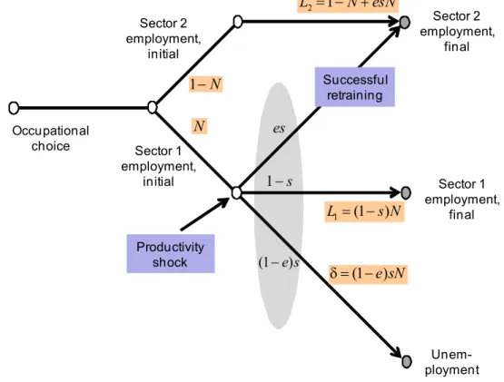
Figure 1 illustrates how retraining leads to reallocation of labor. When the outcome of the productivity shock is unfavorable, employment in sector 1 is terminated, leading to job separation with probability sand continuation with probability 1−s. When fired, the worker can retrain and search for a sector 2 job. When job search is not successful, she remains unemployed. When entering the volatile industry, a worker may thus end up in three states. They ultimately keep their job in sector 1 with probability 1−s, are reallocated to jobs in sector 2 with probability se, and end up unemployed with probability s(1−e). Given independent risks, the ex ante probabilities correspond to ex post fractions. Initial and final labor allocation must satisfy the resource constraint,

L1 = (1−s)N, L2 = (1−N) +esN, δ≡(1−e)sN = 1−L1−L2. (1)

The unemployment rate δ reflects job creation N, firing s in the volatile industry and unsuccessful job search1−efor new employment. Since the unemployment risk is high in the volatile sector 1 and low (zero) in sector 2, the average unemployment rate necessarily reflects the sectoral composition of the economy.

As a result of initial training, sector 1 workers are more skilled and, on average, more productive. Skills are sector specific to some extent so that separation and reallocation leads to a wage loss. Keeping a job in sector 1 earns a higher wage than reemployment,

w1 > wr. We further assume that sector 2 technology is Ricardian with fixed productivities wr > w2. Workers separated from a skill intensive sector 1 job are more productive than those who have spared initial training and started a job in sector 2 right from the beginning. After reallocation, employment in sector 2 consists of 1−N unskilled and

esN retrained workers, earning fixed wages w2 and wr, respectively. If a sector 1 worker becomes unemployed, she generates low income hfrom home production. To sum up, we assume w1 > w_r> w2 > h, where the lower index r indicates re-training.

Sector 1 employment, initial Sector 2 employment, initial Occupational choice Productivity shock Sector 1 employment, final Sector 2 employment, final es N Unem-ployment 1−N 1−s (1−e s) 2 1 L = −N+esN 1 (1 ) L = −s N (1 e sN) δ = − Successful retraining

Fig. 1: Reallocation of Labor

We consider social protection in the context of a possibly progressive wage tax schedule and allow for different proportional tax ratest1,t_randt2in each earnings class with wages w1 > wr > w2. Whilet1 > t2 naturally describes a progressive tax schedule since sector 1 workers on average earn more. Whenevertr < t1, we associate the difference t1−t_r with a wage subsidy. A priori, these tax rates are unrestricted. In addition, the government sets unemployment benefits b, may impose a firing tax ts to reduce job separation and spend on ALMPmto support retraining and assist job search. Taking policy instruments as given, workers decide whether to invest in sector 1 specific skills and, in the event of separation, choose a level of retraining and job search effort. Firms decide whether to employ a worker and, after the productivity shock materializes, whether to close down or continue the employment relationship.

Sector 1 production is organized by risk-neutral firms, each hiring one worker. With perfect competition, firm entry and job creation continue until profits are zero. After hiring, firms are subject to a productivity shock x ∈ [0,∞), leading to output Ax of the job. Once productivity is known, the firm decides whether to continue with earnings

Ax−w1 or close down, fire the worker and accept a loss t_s equal to the firing tax. The firm continues ifAx−w1 −ts. The cut-off productivity is

x1 = (w1−t_s)/A. (2)

When the productivity shock yields a better result x x1, the firm continues the em-ployment relationship, in the other case, the job is terminated. Given a densityg(x)and cumulative distribution G(x), the separation rate is

s(x1) = x1 0 g(x)dx, 1−s(x1)≡ ∞ x1 g(x)dx. (3)

A higher cut-off valuex1 raises the firing rate s and reduces the continuation probability

1−s. Note that 1/s is interpreted as the length of job tenure in the volatile industry. High volatility means a high firing rate and short job duration, i.e. high job turnover.

Entry and job creation give rise to a fixed cost or start-up investment f (see Fonseca et al., 2001). Anticipating the firing decision, firms create jobs if the net present value is non-negative. Define average productivity after entry by xa_≡ ∞

x1 xdG(x) (1−s), π = ∞ x1 (Ax−w1)dG(x)−sts−f = (1−s) (Axa−w1)−sts−f 0. (4) Employment relations also break up when a worker prefers to leave. To prevent this, the firm must pay a high enough wage. Utility of staying in the firm is u((1−t1)w1). Expected utility of leaving and searching for a sector 2 job, subject to unemployment risk, is ue_{, see the next subsection. The firm is able to keep the worker only if the wage} satisfies the participation constraint u((1−t1)w1) ue. We assume productivity and the competitive wage to be high enough so that this constraint is slack.

Job creation under perfect competition pushes up the wage until profits are zero. When firing is optimally chosen as in (2), the derivative of the profit function with respect to

cut-off productivity is zero, dπ =−(Ax1−w1 +t_s)g(x1)dx1 = 0. By the envelope the-orem, dπ/dw1 =−(1−s) anddπ/dts =−s. Hence, the zero profit condition pins down the competitive wage as a function of the firing tax and other fundamental parameters. Solving dπ =−(1−s)dw1 −sdts = 0 yields dw1 dts =− s 1−s, ds dts =−σs, σ≡ g(x1) (1−s)sA. (5)

Hence, a firing tax puts a cost on firms and forces them, in zero profit equilibrium, to cut the wage. For the same reason, the tax also reduces the separation rate.

Sector 2 uses a linear Ricardian technology. Competitive producers pay wages equal to exogenous labor productivities w2 andw_r of a specialized sector 2 worker and a retrained sector 1 worker, and earn zero profits. These wages are fixed constants while w1 is endogenous. Since each firm hires exactly one worker, the number of firms is determined by the number of workers entering sector 1. Since only 1−s new jobs survive, and s

close down, the number of productive jobs (or mature firms) is(1−s)N. Given average productivityxa_{, total sector 1 output X}

1 net of entry costs amounts to

X1 = [(1−s)Axa−f]N, X2 =w2(1−N) +w_resN. (6)

Sector 2 output is produced by two types of workers, specialized sector 2 and retrained sector 1 employees, each generating an output per capita equal tow2 andwr, respectively.

2.2

Labor Market Behavior

There are four realizations of income, yi _{∈ {w}

1, wr, h, w2}. Net of tax income depends on the tax benefit schedule summarized by {t1, t2, t_r, b}. A sector 2 worker earns a safe wage, giving utilityV2 =u((1−t2)w2). A sector 1 worker either keeps her initial job or is fired. When fired, she may retrain and get another job with probability e, or end up unemployed with probability1−e (see Konrad, 2001, for a probabilistic model of human capital investment). Taking account of a utility loss (stigma)χof remaining unemployed,

expected utility of entering sector 1 is

V1 = (1−s)·u((1−t1)w1) +s·ue, (7)

ue _{= max}

e e·u((1−tr)wr) + (1−e)·[u(h+b)−χ]−φ(m)ζ(e).

Henceforth, we define u1 ≡ u((1−t1)w1), u_r ≡ u((1−t_r)w_r), u_h ≡ u(h+b) as well as u2 ≡ u((1−t2)w2) for using as a short-hand. Parameter m illustrates how active labor market policy (ALMP) facilitates retraining by reducing individual effort cost. We assumeφ(0) = 1,φ′

<0< φ′′

andlimm→∞φ(m) =φ0 >0. When the policy is scaled up, it becomes less and less effective. For given m, effort costs are convex increasing, ζ′

> 0 andζ′′

>0, and are assumed strictly positive in the relevant range. The level search effort costs φζ may also be interpreted as ‘stigma of job loss’ because it reduces utility value outside of sector 1 employment while χ reflects a ‘stigma of unemployment’. These two concepts are not the same since a fraction of separated workers successfully retrain but may not enjoy the new job to the same extent.5 _{Finally, the negative cross-derivativeφ}′

ζ′ means that ALMP reduces marginal effort cost and stimulates job search.

The utility cost φζ might also be interpreted asskill specificity since these individuals have previously invested in sector 1 skills and must now retrain to obtain another job in sector 2. Another aspect of skill specificity is the assumption of w1 > wr. A specialized sector 1 worker is not as productive in a sector 2 job after retraining and, as a result, must accept an earnings loss (see Lundquist and Sargent, 1998, on the loss of skills due to unemployment). The effort spent on retraining and job search for employment elsewhere is a matter of incentives. After job separation, individuals choose effort according to

u((1−tr)wr)−u(h+b) +χ=φ(m)ζ ′

(e). (8)

Anticipating subsequent events, workers must decide in the beginning whether to undertake a sector specific skill investment or go to sector 2 right away. Suppose agents

5_{Blanchard and Tirole (2008) and Algan and Cahuc (2009) similarly assume a fixed utility cost of}

unemployment. Since they abstract from reemployment and allow for only one state after separation, they do not differentiate the utility loss from separation

are arranged by the innate abilityn∈[0,1]of performing sector 1 jobs. The discrete effort costi(n)of acquiring sector 1 skills differs by ability according toi′

(n)>0,i(0) = 0and

i(n)→ ∞ forn→1. Lownindicates low effort cost and high ability. Suppose ability is uniformly distributed so that the pivotal valueN ∈[0,1]is also the fraction of individuals with ability n < N. Given that expected utility of entering sector 1 is higher than that in sector 2, V1 > V2, highly able individuals with low cost expect V1 −i(n) > V2 and, thus, invest in a sector 1 specific qualifications. In the other case, type n opts for sector 2 and does not invest. The pivotal agent, identified by the occupational choice condition, determines the initial labor allocation across sectors,

V1−i(N) =V2, V2 ≡u((1−t2)w2). (9)

Initially,N workers opt for sector 1, and1−N go to sector 2. After firing, this allocation is partly revised by retraining, leading to a final allocation L1 and L2 as in (1). If there were no firing (s = 0), there would be no reallocation, L1 = N, and no unemployment. Unemployment results from productivity shocks, frictions in retraining and reallocation which only arise in the volatile industry.

2.3

Equilibrium

Government spends bδ on unemployment benefits and mksN on ALMP, where mk is spending per capita of fired persons in need of a new job. Fiscal budget balance requires

T =t2w2(1−N)+t1w1(1−s)N+t_rw_resN+t_ssN−b(1−e)sN−mksN−C = 0, (10) where C is an exogenous and constant level of other public spending.

Aggregate disposable income stems from earnings of employed and retrained sector 1 workers (first two terms below), benefits collected by unemployed persons, and earnings of specialized sector 2 workers. Since h is income from non-market activity, it does not show up in disposable income,

Using the fiscal budget to replace benefits, profits π = (1−s) (Axa_−w

1)−st_s−f to eliminate w1 and substituting the definitions Xj yields (Y +C+mksN −X1−X2) + πN + T = 0, where the bracket is excess demand. Total demand for market goods includes not only private and public consumption Y +C but also the resource use of ALMP spending. Solving forπ =T = 0 clears the product market by Walras’ Law.

The solution of the untaxed, free market equilibrium is as follows. Parameterswr and

h determine ue_{. Suppose that the lowest possible sector 1 wage, u(w}∗ 1) = u

e_{, implies} positive expected profits π(w∗

1) > 0, reflecting high factor productivity A andxa. This wage also induces a labor allocationN∗

, satisfyingV (w∗

1)−i(N ∗

) =u(w2). Profits attract new firms which bid up the wage ratew1 > w

∗

1. Expected utilityV1 rises, attracting more workers such that N > N∗

satisfying V (w1)−i(N) = u(w2). This process continues until profits are zero, π(w1) = 0. At this equilibrium wage, the participation constraint is not binding, u(w1)> ue. We ‘calibrate’ the model such that w1 > w_r > w2 > h.

3

Optimal Flexicurity

In the present model, policy should address three market distortions, arising from firing externalities, missing private insurance markets, and frictions in retraining and job search. ALMP could be interpreted as a non-rival public good providing market transparancy and public information about employment opportunities that are useful to guide individual training and job search effort and to facilitate transition into new jobs. Or it could be a publicly provided private good such as advice on how to apply for jobs, or subsidized training if new skills are required in alternative occupations. We first analyze how firms and households react to policy changes and than characterize optimal policy.

3.1

Behavioral Effects and Fiscal Impact

Wages and separation rates in sector 1 depend exclusively on the firing tax as in (5), but are independent of the tax benefit schedule for workers. Taking the differential of (7-8)

reveals the policy impact on expected utilityue _{and job search after separation,} due = −u′ r·wredtr+u ′ h·(1−e)db−φ ′ ζ·dm, (12) de = −εr·wredtr−εb·(1−e)db+εm·dm,

where behavioral elasticities are all defined positive,

εr ≡ u′ r eφζ′′ >0, εb ≡ u′ h (1−e)φζ′′ >0, εm ≡ − φ′ ζ′ φζ′′ >0.

In reducing private effort costs, ALMP spending boosts retraining and job search. Taxes and benefits discourage job search and retraining. The tax distortions are measured by the participation tax τE _{≡ t}

rwr +b which consists of the sum of the wage tax plus the benefits lost when an individual switches from unemployment into a job.6 _{Expected utility}

rises with more generous benefit levels and a more intensive ALMP but falls with a higher tax burden on employment.

At the beginning, when seeking employment in sector 1, agents anticipate the separa-tion risk and expect utilityV1 = (1−s)u1+sue. Using ∇ ≡(u1−ue)/u

′ 1, dV1 = u′_h(1−e)sdb−u′_rw_resdt_r−φ ′ ζsdm −u′ 1w1(1−s)dt1−(1−t1− ∇σ)u ′ 1sdts. (13)

After starting employment in the volatile industry, individuals expect to be fired and remain unemployed with probability (1−e)s. Expected utility rises by the marginal welfare gainu′

hdbfrom more generous benefits, scaled by the probability of unemployment. Other taxes and benefits are interpreted similarly. More intensive ALMP becomes useful in the event of job separation which is expected with probabilitys. Importantly, a higher firing tax affects workers via two offsetting channels and leaves an a priori ambiguous net effect. On the one hand, the tax reduces firing by ds = −σsdts which boosts expected utility by∇u′

1(−ds) = (u1−ue) (−ds). Less firing allows workers to enjoy more often high utilityu1 from sector 1 employment instead of low utilityue as expected after separation.

6_{The participation tax is implicit in (8). To see this, substitute the Taylor expansion u}

r = uh+ u′

h[(1−tr)wr−b−h]and note the definition ofτ E , yieldingwr−τ E −hu′ h+χ=φζ ′_(e).

On the other hand, the tax reduces the gross wage by dw1 =−₁₋s_sdts. Since this occurs with probability 1−s ex ante, expected welfare declines by(1−s)u′

1(1−t1)dw1. The willingness to pursue employment in the volatile industry and invest in sector specific skills depends on expected utilityV1 relative to welfareV2 =u((1−t2)w2) from a safe sector 2 job. Taking the differential of the occupational choice condition in (9) yields the entry response,

dN = −η1w1(1−s)Ndt1−η_rwresNdtr+ηh(1−e)sNdb

−ηssNdts+ηmsNdm+η2w2(1−N)dt2,

(14)

where entry elasticities are defined positive,

η1 ≡ u′ 1 N i′, η2 ≡ u′ 2 (1−N)i′, ηm ≡ − φ′ ζ Ni′, ηr ≡ u′ r N i′, ηh ≡ u′ h Ni′, ηs≡(1−t1− ∇σ)η1.

A higher taxt2 on sector 2 earnings pushes workers into sector 1 employment. Conversely, all policies raising the present value of net taxes on sector 1 earnings discourages employ-ment in the volatile sector. Clearly, higher unemployemploy-ment benefits reduce the present value ofnet taxes and, thus, make volatile employment more acceptable. More intensive ALMP improves labor market prospects in the event of job separation and, thus, similarly encourages sector 1 employment.

Employment effects on different margins determine the tax yield and the net result on the fiscal constraint in (10). In the present model, all labor market effects are dis-crete in the sense of people switching from one state to another, either via disdis-crete skill investment dN, job separation ds or retraining with successful job searchde. For each of these margins, we define effective tax rates τN_{, τ}S _andτE_{, which capture the impact of} behavioral changes on net tax revenue,

dT = (1−N)·w2dt2+ (1−s)N ·w1dt1+esN·w_rdt_r+ (1−t1)sN ·dt_s

−(1−e)sN ·db−ksN ·dm+τN _{·dN +τ}S_·Nds+τE _·sNde, (15) where effective tax rates on the extensive margins of employment are defined as

Using these rates, we can write the GBC as T = t2w2 +τNN = 0. If one more person switches from sector 2 employment into sector 1, net tax revenue rises by τN_. The net impact consists of the differential tax liability of sector 1 over sector 2 employees plus the additional net tax revenue τS _{that is collected when a sector 1 worker gets} fired, an event which occurs with probability s. The ‘effective’ firing tax τS _{captures the} fiscal consequences of job separation. It consists of the firing tax paid by firms, plus the average net tax liability of a worker after separation, equal to etrwr −(1−e)b, minus spending km on ALMP per capita of a fired worker, minus the foregone tax t1w1 when this person is no longer employed in sector 1. Writing the net tax liability after separation as etrwr−(1−e)b=eτE−breveals the fiscal gain τE of putting one more person back to work, consisting of the wage taxtrwr of this reemployed person plus the savings in UI spending when the same person no longer collects benefits.

Using these effective tax rates and substituting the behavioral changes given above yields a change innet fiscal revenue equal to

dT = 1 +τN_η 2 w2(1−N)dt2+ 1−τN_η 1 w1(1−s)N dt1 +1−τN_η r−τEεr wresNdtr− 1−τN_η h+τEεb (1−e)sNdb +1−t1−τSσ−τNη_s sN dts− k−τN_η m−τEεm sNdm. (16)

For example, spending on more intensive ALMP rises by k·sN dm which obviously is a loss of net tax revenue. Since the policy attractsη_msNdm more workers to sector 1 as in (14), and each one adds τN _{in expected value to the government budget, net tax revenue} rises by τN_η

msNdm. The budget further improves since ALMP brings a larger portion of all fired persons back to work and raises the number of reemployed sector 1 workers byεmsNdm. Each of these persons who were previously unemployed and now get a job, pays tax and stops claiming benefits, adding τE _{to the budget. Adding up all these} con-sequences, the net fiscal cost of more intensive ALMP is onlyk−τN_η

m−τEεm

sNdm

instead ofksNdm. The difference reflects self-financing due to the beneficial labor market consequences of the policy.

3.2

Welfare Optimal Policy

Expected utility ex ante, prior to entry, equals average welfare ex post. An optimal policy maximizes social welfareV = maxt1,tr,b,ts,m,t₂NV1+ (1−N)V2−

N

0 i(n)dn+λT where λ is the Lagrange multiplier relating to the fiscal constraint T = 0. Due to occupational choice, a variation of N yields dV = (V1−V2−i)dN = 0. Welfare maximization thus implies dV =NdV1+ (1−N)dV2+λdT = 0. Substituting (13) and (16) yields

dV /dt1 = − u′ 1− 1−τNη1 λw1(1−s)N = 0, dV /dtr = − u′ r− 1−τNηr−τ E εr λwresN = 0, dV /db = u′ h− 1−τNηh+τ E εb λ(1−e)sN = 0, (17) dV /dts = − (1−t1− ∇σ)u ′ 1− 1−t1−τSσ−τNη_s λsN = 0, dV /dm = −φ′ ζ−k−τNηm−τ E εm λsN = 0, dV /dt2 = − u′ 2− 1 +τNη2 λw2(1−N) = 0.

Taking ratios to eliminate the shadow price λ leaves five optimality conditions which, together with the fiscal constraint, implicitely determine the optimal values of the six unknown policy variables.

Consider first unemployment insurance (UI) of dismissed workers. Dividing the second and third conditions yields

u′ r u′ h = 1−τ N_η r−τEεr 1−τN_η h+τEεb <1. (18)

The left side reflects the marginal rate of substitution between consumption in the reem-ployed and the unemreem-ployed state (equal to − e

1−e u′_r

u′

h) which indicates how much extra

consumption an agent would need in the bad state to compensate for one unit given up in the good state. The right side is proportional to the marginal rate of transformation (equal to the fraction times − e

1−e) which states the rate at which government can shift consumption from the good to the bad state. If effort were inelastic (ε-elasticities zero), optimal policy would implement full consumption smoothing between retraining and un-employment, u′

r =u ′

45◦

-line in the right panel of Figure 2 where consumption in each state is denoted bycj, i.e.

cr = (1−tr)wr. However, insurance diminishes incentives for job search and retraining. Providing insurance becomes more costly when it contributes to higher unemployment. It inflates social spending and simultaneously looses tax revenue when an agent switches from work to unemployment. The net effect on the fiscal budget is proportional to the participation tax τE _{in both cases. Given that insurance becomes more costly, optimal} policy advises limited insurance, leaving an income gap (1−tr)wr > b+h and u′r< u

′ h. b

C

C

C

u

1

V

1

e

e

−

−

C

Fig. 2: Insurance and Job Search

We have assumed that job separation in the volatile industry leads to a depreciation of sector specific skills. In consequence, the next best job opportunity pays only a lower wage,w1 > wr. In other words, firing leads to an uninsured wage loss even if another job is found. Policy should thus provide to some extentinsurance for earnings risk which is different from UI. Dividing the first and second conditions yields

u′ r u′ 1 = 1−τ N_η r−τEεr 1−τN_η 1 <1. (19)

Without moral hazard in UI (εr = 0), optimal policy aims at complete consumption smoothing between primary and reallocated employment, u′

1 = u ′

(1−t1)w1 = (1−t_r)wr. Full insurance requires a progressive rate structure, t1 > tr. If there is moral hazard, it becomes optimal, for given UI benefits, to strengthen incentives for retraining by shifting relatively more income towards reallocated employment. This calls for a higher tax rate on primary employment and an even more progressive tax system. With optimal policy, we thus have (1−t1)w1 < (1−t_r)wr. The left panel of Figure 2 illustrates.7

Another policy concern is redistribution between sector 1 workers who are in well paying, but risky jobs, and sector 2 workers where wages are safe but low (we assumed

w1 > w_r > w2 > h). Dividing the first and last conditions yields u′ 1 u′ 2 = 1−τ N_η 1 1 +τN_η 2 <1. (20)

Clearly, if the skill distribution were exogenous and a result of pure luck, ηj = 0, and investment in sector 1 skills were thus completely inelastic, optimal policy would also implement full redistribution, u′

1 = u ′

2 and (1−t1)w1 = (1−t2)w2. Due to w1 > w2, and ignoring for the moment other taxes and spending, the fiscal constraint t1w1N + t2w2(1−N) = 0requires a tax on sector 1 workers and a transfer t2 to sector 2 workers. In general, we can write the fiscal budget as t2w2 = −τNN where the effective tax τN on sector 1 workers finances a transfer t2w2 <0 to sector 2 workers. Imperfectly elastic skill investment prevents perfect income smoothing since such redistribution dimishes incentives for initial skill investment and, thus, becomes increasingly costly. Hence, with positive η-elasticities, u′

1 < u ′

2 and(1−t1)w1 >(1−t2)w2.

The government may use a firing tax to implement an optimal degree of job protec-tion. Notingηs≡(1−t1− ∇σ)η1, the first and fourth conditions yield

τS _{=∇= (u}

1−ue)/u ′

1 ⇒ ts=t1w1+ [(1−e)b−t_rw_re] +km+∇. (21) The firing tax performs the same role as in Blanchard and Tirole (2008), even though the tax has new redistributive implications and additionally affects job creation and hiring. Its

7_{We assume that a job loss reduces utility so much that the participation constraintu}

1> u

e

is slack. With full consumption smoothing,u1=ur=uh, the utility loss,u₁−u

e

= (1−e)χ+φζ(e)is positive ifζandχ are positive, whereeis determined byχ=φζ′_(e).

purpose is to internalize negative firing externalities. When dismissing a worker, the firm imposes an income equivalent utility loss ∇ on that person. In addition, creates a fiscal externality consisting of several components. First, there is one person less paying the tax

t1, and there is one person more who collects on average a net subsidy (1−e)b−trwre, and there is extra spendingkm per capita on ALMP. All these components might justify a substantial level of the firing tax.

Finally, active labor market policy(ALMP) can usefully complement other instru-ments. In raising m, the government spends a larger amount km per capita of the sN

dismissed workers who are in need to be reallocated to another job. Dividing the fifth by the first condition, noting ηm = (−φ

′

ζ/u′

1)η1 and rearranging yields8 due_/dm du1/dc1 = −φ ′ ζ u′ 1 =k−τE_ε m. (22)

The left side states the marginal benefit of ALMP which raises expected utility ue _{of a} fired relative to a retained worker. The social cost of ALMP consists of the marginal resource cost k per capita and is reduced by the budget savings τE_ε

m if ALMP puts a larger fraction of fired workers back to work. The elasticity εm measures how effective ALMP is to support job reallocation and boost reemployment among dismissed workers. The budget savings are proportional to the participation tax τE _{= t}

rwr+b. Immervoll et al. (2007) found participation tax rates in Europe to vary mostly between 50 to 70% of gross wages, and up to 80% in Nordic countries. The upshot is that the participation tax and, in turn, the fiscal savings from ALMP are large in a generous welfare state with high benefits. These savings reduce the social cost of ALMP and lead to larger programs. ALMP programs thus become an essential ingredient of an advanced welfare state.

Finally, to put our analysis of flexicurity into perspective, we reproduce two central results of Blanchard and Tirole (2008), henceforth BT, as a special case of the present

8_{ALMP is productive sincedu}e

/dm=−φ′_{ζ >0by the envelope theorem. Instead of reducing search}

cost, ALMP could raise earnings on the next job, w′

r(m)>0, which boosts search and utility as well, due

/dm =e(1−tr)w′ru′r >0. However, a purely sanctions based system which reduces utility during

unemployment, e.g. χ′_{(m)>0, cannot be part of an optimal program sincedu}e

model. Excluding entry and job creation, we fix the mass of sector 1 workers at N = 1. Further, BT abstracted from job reallocation so that e = 0 and firing always results in unemployment. With these margins fixed, the ε- and η-elasticities are all zero. Social welfare isV1 = (1−s)u1+s(uh−ζ). The fiscal constraint reduces toT =t1w1(1−s) +

(ts−b)s=t1w1+sτS = 0, whereτS ≡t_s−b−t1w1 is the effective firing tax, or subsidy. The optimality conditions in (17) with respect to t1, band ts are reduced to

u′

1 =λ=u ′ h, τ

S _{=∇. (23)}

The optimal policy in BT assures full consumption smoothing (1−t1)w1 = λ = h+b. The stigma ζ of a job loss thus leads to a utility differential between work and unemployment equal to ∇ = (u1−uh+ζ)/u′1 =ζ/u

′

1. Now suppose first that stigma is absent, so that τS _{=∇= 0. The fiscal constraint t}

1w1 =−sτS then implies t1 = 0, and ts =b. Benefits are exclusively financed with a firing tax with no other tax on wages. Full consumption smoothing implies w1 = h+b. Substituting this into (2) leads to a firing thresholdAx1 =w1−ts =h+b−ts =h, i.e. Ax1 =has in Proposition 1 of BT. If there is a positive stigma, the effective firing taxτS _{=∇is positive, implyingt}

s =b+t1w1+∇. The fiscal budget leads to a wage subsidyt1w1 =−s∇<0. Substitutingts into the firing rule and noting full insurance yields Ax1 =h− ∇< h. If there is stigma of job loss, the firing externality becomes larger. Optimal policy thus raises the firing tax to reduce job separation. Since this also depresses wages, workers are compensated by an employment subsidy t1w1 <0. These results replicate Proposition 2 of BT.

4

Policy Reform

In optimizing a social welfare function reflecting the allocative and distributive goals of public policy, the last section has derived an optimal flexicurity policy as part of the overall tax benefit schedule. The optimal policy with six policy instruments, t1, t_r, b, t_s, m and t2, is only implicitely determined by six conditions, i.e. (18-22) together with the fiscal

constraint. This section considers piecemeal reform. We aim to show how a small policy reform implementing steps towards an optimal policy leads to beneficial labor market and sectoral adjustment and, thereby, promises welfare gains. The first experiment starts out with an untaxed, free market equilibrium and introduces a flat rate UI scheme where all workers pay the same proportional contribution rate to finance benefits of unemployed workers. This experiment resembles most current UI schemes which have largely flat contribution rates and often contain cross-subsidization between groups with different unemployment risks. In subsequent scenarios, we ‘improve’ on this scheme by adjusting the structure of tax rates and by complementing the tax benefit schedule with ALMP and with job protection by means of a firing tax. All scenarios must fulfill the fiscal constraint in (16),dT = 0, where effective tax rates are defined in (15). Inserting the welfare change of sector 1 employees in (13), social welfare changes by dV =NdV1+ (1−N)dV2, or

dV = −u′ rwresNdtr−u′1w1(1−s)Ndt1−u′2w2(1−N)dt2 +u′ h(1−e)sNdb−φ ′ ζsNdm−(1−t1− ∇σ)u ′ 1sNdts. (24)

Flat Unemployment Insurance: Suppose the government finances benefits with a

flat tax, t1 = t_r = t2 = t, and abstains from any other labor market intervention, i.e. ts =m = 0. Since there are gains from insurance, the policy must be welfare improving, at least if it is operated at a small scale. In this experiment, the wage structure is exogenous to the policy change since the wage w1 is fixed by ts = 0. Starting from a free market equilibrium with zero taxes implies τj _{= 0. Financing small UI benefits and} satisfying the constraint in (16) requires a small increase in the uniform tax rate of

Γdt= (1−e)sNdb, Γ≡w1(1−s)N +w_resN+w2(1−N), (25) whereΓis the tax base consisting of average wage earnings of individuals in different jobs. Substituting into the welfare differential and evaluating at t=b= 0 yields

dV dt b=0 = 1− u ′ 1 u′ h w1(1−s)N Γ − u′ r u′ h wresN Γ − u′ 2 u′ h w2(1−N) Γ Γu′ h >0. (26) The income distribution is characterized by w1 > w_r > w2 > h, implying marginal rates of substitution all smaller than one. Since the weights of these ratios add up to unity, the

square bracket is positive. Offering small UI clearly raises welfare when private insurance markets are missing. Since tax distortions are initially small, the gains from insurance more than justify the tax cost.

The flat UI scheme, by assumption, does not make use of the firing tax, so that the wage and the separation rate in the volatile industry, w1 and s, remain constant. Substituting (25) into (12) shows that the policy reform diminishes employment,

de/dt=−[ewrεr+ (Γ/sN)εb]. (27)

Clearly, UI benefits and the contribution tax discourage retraining and search effort so that job reallocation slows down and unemployment among dismissed workers rises.

Substituting the fiscal balancing rule stated above into the entry response in (14) and noting the definition of Γ yields

dN/dt= (ηh −η1)w1(1−s)N + (η_h−η_r)wresN+ (ηh+η2)w2(1−N)>0. (28)

The impact is unambiguously positive since w1 > w_r > h implies u ′ 1 < u ′ r < u ′ h and, therefore, η1 < η_r < η_h, when evaluated in the initial untaxed equilibrium. The policy implicitely cross-subsidizes from sector 2 to sector 1 workers and, thus, encourages more people to enter the volatile industry. Entry results from occupational choice and is driven by V1−i(N) = V2. Raising the tax rate clearly reduces utility from sector 2 work since the policy extracts tax from sector 2 workers without any compensation. Sector 1 workers also pay tax when employed, but are offered benefits when unemployed. In net terms, sector 1 workers benefit from cross-subsidization so that expected utility V1 rises. Both effects stimulate investments in sector 1 skills and encourage entry.

Aggregate unemployment reflects job creation as well as firing and job search. The unemployment rate is δ = (1−e)sN. Given a constant firing rate, the scenario changes unemployment bydδ=−sNde+(1−e)sdN >0. More entry exposes a larger fraction of the population to unemployment risk. Further, reallocation of dismissed sector 1 workers slows down and a larger share of them ends up unemployed. Both factors contribute to

more unemployment. Since occupational choice determines the economy’s sectoral compo-sition, the impact of entry on the unemployment rate also reflects structural change which shifts employment from stable to highly volatile sectors or, equivalently, from sectors with low to sectors with high unemployment incidence. Thereby, the aggregate unemployment rate is a function of the economy’s sectoral structure.

We now perform further policy experiments, assuming that a flat UI scheme is in place but no other tax or labor market policy is used. The result of this first experiment is that the participation tax on dismissed workers is relatively large,τE _≡tw

r+b > 0. In contrast, even though there is no statutory firing tax, ts = 0, the effective tax on firing is negative,

τS _{≡ [etw}

r−(1−e)b]−tw1 < 0, since UI among dismissed workers is cross-subsidized by other groups so that the square bracket is negative. If UI were strictly limited to dismissed workers, insurance would be actuarially fair,etwr = (1−e)b. Given a negative effective tax τS_{, the flat UI scheme ends up subsidizing firing of workers in the volatile} industry. Firing thus leads to a loss in the fiscal budget proportional to τS_{. Finally, the} policy cross-subsidizes from sector 2 to sector 1 workers and, thereby, encourages entry and job creation in sector 1. This is seen by the fiscal constraint T = tw2 +τNN = 0, which implies τN _{< 0 when t > 0. With τ}N _{= tw}

1−tw2 +sτS negative, the effective firing tax τS _{must actually be strongly negative.}

Sectoral Redistribution: The flat tax rate structure to finance UI does not satisfy the distributional concerns in policy making. Given concave utility and the fact that earnings are lower in sector 2, a welfare based policy calls for redistribution from sector 1 to sector 2, and not vice versa. Starting from the flat UI scheme, this experiment raises the tax rate on sector 1 workers to cut the tax burden on low wage earners in sector 2. By (16), budget balance dictates a higher tax rate on sector 1 employees when t2 is reduced,

w1(1−s)Ndt1 =− 1 +τN_η 2 1−τN_η 1 w2(1−N)dt2. (29)

The flat UI scheme redistributes towards sector 1, τN _{<0, which is the ‘wrong’ direction.} Evaluating (24) shows how redistribution towards sector 2 boosts welfare,

dV =− u ′ 2 u′ 1 −1 +τ N_η 2 1−τN_η 1 u′ 1w2(1−N)dt2. (30) Since w1 > w2, the square bracket is clearly positive. Hence, starting from a flat scheme and moving towards a more progressive rate structure (dt1 > dtr = 0 > dt2) is welfare improving. Since this policy reform keeps not only ts =m = 0 constant but also tr and

b, it has no impact on the separation rate s and on job search and labor reallocation e. The only effect is on entry and job creation. Evaluating (14) subject to (29) yields

dN = η2+η1 1 +τN_η 2 1−τN_η 1 w2(1−N)dt2 <0. (31) Both the lower tax rate on sector 2 and the higher rate on sector 1 employment discourage entry and employment in the volatile industry. Since neither the firing rate nor the rate of job reallocation are affected, the policy also squeezes aggregate unemployment,

dδ = (1−e)sdN <0. When a smaller part of the population gets employed in the volatile sector, a smaller part is subject to unemployment risk. Structural change contributes to lower unemployment when sectors with high unemployment rates shrink and sectors with a low unemployment incidence expand.

Subsidizing Job Reallocation: While redistribution calls for a progressive tax struc-ture (t1 > t2), the government might want to reduce the effective rate t_r below t1 by complementing the wage tax schedule with special tax credits or wage subsidies to reem-ployed workers in order to encourage retraining, thereby reducing the ratetr belowt1. In fact, the tax schedule might actually become non-monotonic witht1 > t2 > tr in spite of

w1 > w_r > w2 as it clearly does in the optimal policy scenarios of the next section. The rationale of this policy rests on the following arguments. Wage taxes and UI discourage retraining and job search of fired workers and reduce the transition rateeinto alternative employment. When switching from unemployment into a job, individuals face a very high participation tax τE_{. Bringing down the participation tax and thereby encouraging} re-training and job search helps to speed up job reallocation. Since high benefits are needed

to provide insurance, the only way to do so is the reduce the tax ratetr. This motivates a reform shifting the tax burden from reemployed workers, the middle income wage earners in our model, towards the top (and bottom) income class,

w1(1−s)Ndt1 =− 1−τN_η r−τEεr 1−τN_η 1 wresNdtr. (32)

Starting from the flat tax benefit schedule, the policy boosts welfare by

dV =− u ′ r u′ 1 − 1−τ N_η r−τEεr 1−τN_η 1 u′ 1wresNdtr. (33) Since u′ r > u ′

1 and ηr > η1 in the initial equilibrium with a flat scheme, the square bracket is clearly positive. Hence, raising t1 to finance a budget neutral tax cut for reemployed workers, dtr < 0, boosts welfare. Since firing depends neither on t1 nor on tr, the separation rate is unchanged. However, the cut in the participation tax stimulates job search and reemployment of dismissed workers byde =−εrwredtr. Substituting (32) into (14) and notingηr/η1 =u

′ r/u ′ 1 yields dN =− u ′ r u′ 1 − 1−τ N_η r−τEεr 1−τN_η 1 η1wresNdtr. (34)

By the same argument as before, the lower tax on reemployed workers, dtr < 0 < dt1, boosts entry and employment in the volatile industry. The effect on aggregate unemploy-mentδ = (1−e)sN is ambiguous since 1−e falls whileN rises.

Job Protection: The next reform introduces job protection to complement the flat UI scheme. Since the firing tax is an extra cost, sector 1 firms compete down the wage to break even in zero profit equilibrium. To compensate workers, the scenario cuts the tax rate t1 subject to fiscal budget balance,

w1(1−s)Ndt1 =− 1−t−τS_σ−τN_η s 1−τN_η 1 sN dts. (35)

Substituting into the welfare change stated in (24) and usingηs= (1−t1− ∇σ)η1 yields dV =u′ 1 ∇ −τS 1−τN_η 1 σsNdts. (36)

Job protection reduces turnover,ds=−σsdts, so that workers are exposed less frequently to the utility loss ∇u′

1 =u1−ue. The firing tax, however, leads to an a priori ambiguous effect on disposable income of sector 1 employees. Since the flat UI scheme subsidizes firing, i.e. τS _{<0, the reduced job separation yields a fiscal dividend in proportion to τ}S which allows a relatively larger tax cut t1. Disposable earnings and welfare increase on this account. However, the tax also forces firms to cut the gross wage. Depending on the size of the tax cut relative to the wage reduction, the net of tax wage may rise or fall. Using (35) and (5), and making use of ηs = (1−t1 − ∇σ)η1, yields

d[(1−t1)w1] = ∇τN_η 1 −τ S 1−τN_η 1 σs 1−sdts. (37)

Sector 1 employees benefit from job protection since τS _{< 0 at the outset. Despite of a} lower gross wage, the compensating tax cut more than offsets this income loss, i.e. u1 rises while ue _{remains constant. The introduction of a firing tax clearly boosts welfare.}

Entering sector 1 thus promises higher expected welfare which induces more workers to invest in sector specific skills and allows the volatile industry to expand employment. Evaluating (14) and using the same steps as before results in

dN = ∇ −τ S 1−τN_η 1

ση1sNdts. (38)

Shifting labor to the volatile sector inflates unemployment δ = (1−e)sN since unem-ployment is concentrated there. Hence, joblessness rises with the expansion of the volatile industry while a lower separation rate reduces unemployment. Since the reemployment rate e is constant in this scenario, unemployment changes by dδ = (1−e) [sdN +Nds]. Substituting the change in entry and job separation yields an ambiguous net effect of

1 (1−e)σsN dδ dts =− 1− ∇ −τ S 1−τN_η 1 sη1 =−1−(∇s+tw1−tw2)η1 1−τN_η 1 , (39)

where the second equality uses τN _=tw

1−tw2+sτS. To identify the conditions favoring a rise or fall in unemployment, one may interpret a large ∇ = (u1−ue)/u

′

1 as a high degree of sector specificity of skills. High sector specificity means that a worker suffers a large loss in wage and utility ∇ when loosing her job. Further, a high separation rate s

stands for short employment tenure and high job-turnover, characterizing a very volatile industry. Finally, a large value ofη1 means that entry into sector 1 is very elastic.

Starting with a flat UI scheme, a small firing tax changes the unemployment rate as in the last term above. If sector 1 is characterized by a large degree of sector specificity of skills (∇ large), high job turnover (large s), and elastic labor supply (highη1, reflecting elastic entry), a firing tax combined with a budget neutral wage subsidy (dts >0> dt1) could actually raise unemployment. The reason is that all these conditions favor entry and a large expansion of the volatile industry where the sectoral unemployment rate is high, while the stable sector with a low (zero) unemployment rate strongly shrinks. The resulting increase in the unemployment rate could dominate the reduction in unemploy-ment on account of a lower separation rate. However, this is not possible when the firing tax is close to its optimal value, implying∇=τS_{, and is further increased.}9 _{In this case,}

the unemployment rate unambiguously falls, see the first equality above.

Active Labor Market Policy: Finally, we analyze the consequences of complementing the flat UI scheme by introducing ALMP to facilitate retraining, search and job reallo-cation. Again, we raise the wage tax of workers in the volatile industry since the policy benefits them by improving their labor market prospects if they get fired. Spending more an ALMP by raisingm thus requires a higher tax on sector 1 employees,

w1(1−s)N dt1 = k−τN_η m−τEεm 1−τN_η 1 sNdm. (40)

Welfare rises if the gains from better labor market prospects after firing dominate the welfare loss from a higher tax on sector 1 employment. Using η_m = −φ′

ζη1/u ′

1 yields a welfare change that is related to the optimality condition in (22),

dV = −φ ′ ζ u′ 1 −k−τE_ε m u′ 1 1−τN_η 1 sNdm. (41)

Whether ALMP is welfare improving depends on its potency to raise expected utility of fired workers, due_{/dm = −φ}′

ζ > 0, relative to its cost, k−τE_{εm. Obviously, if it is}

too costly (k high), the policy reduces welfare and is not advised. However, if high UI benefits are offered to insure workers, the participation taxτE _{is high and the policy yields} large fiscal gains. In bringing more people back to work, the policy boosts tax revenue and contains social spending. Hence, the net fiscal cost of ALMP is greatly reduced in the presence of a large welfare state. This is even more the case if the policy is very effective in reallocating workers, as indicated by a large elasticityεm. Given that ALMP is sufficiently productive, it becomes an essential ingredient of the welfare state.

ALMP boosts job search byde =εmdm. Given a constant firing taxts, the separation rate remains unchanged. If the policy boosts welfare, it also encourages entry. Imposing budget balance and using ηm =−φ

′

ζη1/u ′

1 yields an entry response in (14) equal to

dN = −φ ′ ζ u′ 1 −k−τE_ε m η1 1−τN_η 1 sNdm. (42)

ALMP cannot influence unemployment via the firing channel since s is fixed in this sce-nario. On the positive side, ALMP clearly speeds up job reallocation and reduces the unemployment risk after a job loss. However, by encouraging entry into the volatile sector, it also raises the absolute levels of job separation which adds to unemployment

δ= (1−e)sN. The net effect is a priori ambiguous. However, if ALMP is at its optimal level, the square bracket is zero and ALMP does not affect entry and sectoral composition at the margin. In this case, ALMP reduces unemployment by stimulating job search.

5

Comparative Statics of Optimal Policy

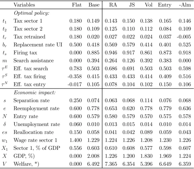
This section numerically illustrates our results and shows how optimal flexicurity changes with risk-aversion, volatility and behavioral elasticities. In all cases, we recalibrate the model to yield the same data. Column ‘Flat’ in Table 1 reports equilibrium values when policy is not optimized and neither a firing tax nor ALMP are used. The tax schedule is flat with a rate of 18%. Revenues finance public consumption equal to 15% of GDP, and UI benefits. Public goods per capita are fixed and, thus, do not affect welfare analysis.

Initially, 60% of the labor force train to become employed in the volatile sector where the separation rate is 25%.10 _{After separation, 60% get reemployed in the safe sector, the rest}

ends up unemployed. Unemployment amounts to 6%, reflecting job creation (entry), job destruction (firing) and the frictions in job reallocation (search). Ultimately, only 45% of the workforce remain employed in the volatile industry and 49% end up in the safe sector. The gdp share of the volatile sector is about 55%.

Variables Flat Base RA JS Vol Entry -Alm

Optimal policy: t1 Tax sector 1 0.180 0.149 0.143 0.150 0.138 0.165 0.146 t2 Tax sector 2 0.180 0.109 0.125 0.110 0.112 0.084 0.109 tr Tax retrained 0.180 0.020 0.027 0.022 0.024 0.037 -0.005 br Replacement rate UI 0.500 0.418 0.569 0.579 0.414 0.401 0.525 ts Firing tax 0.000 0.885 0.946 0.917 0.861 0.873 0.918 m Search assistance 0.000 0.394 0.264 0.126 0.392 0.383 0.000

τE _{Eff. tax search 0.783 0.503 0.686 0.691 0.503 0.503 0.598}

τS _{Eff. tax firing -0.358 0.415 0.433 0.433 0.414 0.409 0.516}

τN _{Eff. tax entry -0.017 0.105 0.078 0.104 0.102 0.150 0.106}

Economic impact: s Separation rate 0.250 0.074 0.063 0.068 0.114 0.076 0.068 e Reemployment rate 0.600 0.778 0.653 0.620 0.778 0.779 0.636 N Entry rate 0.600 0.579 0.580 0.579 0.570 0.575 0.578 δ Unemployment rate 0.060 0.010 0.013 0.015 0.014 0.010 0.014 es Reallocation rate 0.150 0.058 0.041 0.042 0.089 0.059 0.043

w1 Wage rate sector 1 1.400 1.229 1.224 1.226 1.208 1.230 1.226 X1 Sector 1, % of GDP 0.556 0.603 0.610 0.608 0.577 0.598 0.607 X GDP, %) 0.000 2.008 1.226 1.200 1.830 1.969 1.224

V Welfare, *) 0.000 6.492 7.365 6.354 5.396 6.649 6.359 Legend: All values in absolute terms, %) change in percent. *) Welfare change in percent

of initial GDP,100∗(V−V0)/X0. (FLAT): flat tax rate and no welfare policy. (BASE):

policy with base line parameters ρ= 1.75,ǫ= .4, var(x) = 3 and η =.8. (RA): high

value of risk-aversion ρ = 3. (JS): low elasticity of job search ǫ = .2. (VOL): high

volatilityvar(x) = 5. (ENTRY): low elasticity of entryη=.4. (-ALM): no active labor

market policy m= 0.

Table 1: Comparative Statics of Optimal Welfare Policy

Column ‘Base’ reports the consequences of fully optimizing flexicurity and tax policy. Note first the effective tax rates in the status quo as defined in (15). The effective tax on job search is a high .78 which amounts to 68% of a retrained worker’s wage (τE_/w

r=.68, which is the sum of the tax rate and UI replacement rate). Such high values are consistent with the calculations of participation tax rates in Europe by Immervoll et al. (2007). More surprisingly, the status quo involves a high firing subsidy equal to τS _=−.35which amounts to about 25% (= τS_/w

1) of a worker’s salary. This subsidy consists of the tax loss from each person that is fired (t1w1 =.25) plus the net budget cost of a fired worker (equal to etrwr−(1−e)b = −.1). Firing imposes a substantial net cost on the fiscal budget. Finally, the initial flat tax equilibrium also involves a small entry subsidy τN_. Although the tax liability of sector 1 workers exceeds that in sector 2 byt·(w1 −w2), this net entry tax is more than offset by the firing subsidy sτS _{that sector 1 workers receive} whenever they loose their job.

With baseline parameter values, moving to a fully optimized policy leads to several adjustments of instruments. First, reflecting distributional concerns, the government moves to a progressive wage tax schedule by raising the tax rate on high sector 1 earnings relative to the tax rate on lower sector 2 earnings, t1 > t2. Second, it strongly reduces the tax rate t2 to encourage job search and retraining after separation from sector 1 employment. The difference t1 −tr may be interpreted as a wage subsidy to facilitate job reallocation. Third, and for the same reason, the government reduces unemployment benefits of dismissed workers, leading to a lower replacement rate of .41 instead of .5 initially. This means that the initial replacement rate was too high, given the degree of risk-aversion. As a result, the effective tax on job search is much reduced from .78 to .5. Fourth, the government imposes a large firing tax to internalize the negative firing externalities which turns the effective subsidy of−.36into an effective tax on firing equal to

.4. In consequence, the separation rate is strongly reduced from 25 to 7% of initially hired workers which, in turn, reduces the reallocation ratees despite of a higher reemployment rate e among fired workers. The firing tax also raises significant public revenues and contributes to an overall lower tax burden. Fifth, the government also introduces an