A Data-driven Building Seismic Response Prediction Framework: from Simulation and Recordings to Statistical Learning

(1)

Permalink https://escholarship.org/uc/item/4b56h24z Author SUN, HAN Publication Date 2019 Peer reviewed|Thesis/dissertation

eScholarship.org Powered by the California Digital Library

(2)

UNIVERSITY OF CALIFORNIA Los Angeles

A dissertation submitted in partial satisfaction of the requirements for the degree Doctor of Philosophy in Civil Engineering

by

Han Sun

(3)

(4)

ii

ABSTRACT OF THE DISSERTATION

by

Han Sun

Doctor of Philosophy in Civil Engineering University of California, Los Angeles, 2019

Professor John Wright Wallace, Chair

Structural seismic resilience society has been grown rapidly in the past three decades. Extensive probabilistic techniques have been developed to address uncertainties from ground motions and building systems to reduce structural damage, economic loss and social impact of buildings subjected to seismic hazards where seismic structural responses are essential and often are retrieved through Nonlinear Response History Analysis. This process is largely limited by accuracy of model and computational effort. An alternative data-driven framework is proposed to reconstruct structure responses through machine learning techniques from limited available sources which may potentially benefit for “real-time” interpolating monitoring data to enable rapid damage assessment and reducing computational effort for regional seismic hazard assessment. It also provides statistical insight to understand uncertainties of seismic building responses from both structural and earthquake engineering perspective.

(5)

iii The dissertation of Han Sun is approved.

Henry J. Burton

Ali Mosleh

Jonathan Paul Stewart

John Wright Wallace, Committee Chair

University of California, Los Angeles, 2019 2019

(6)

iv

To my parents …

(7)

v

List of Figures

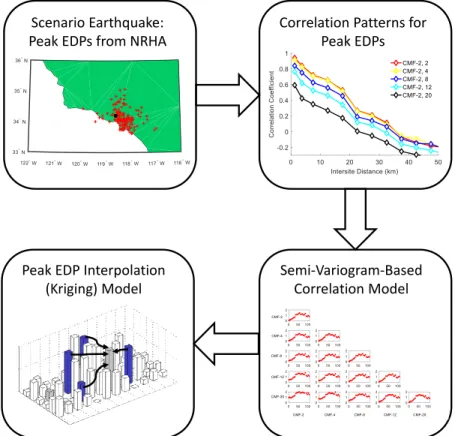
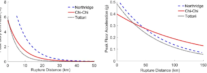
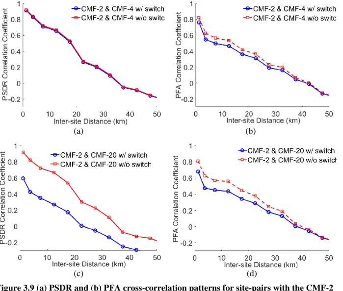
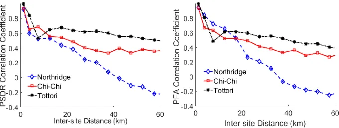
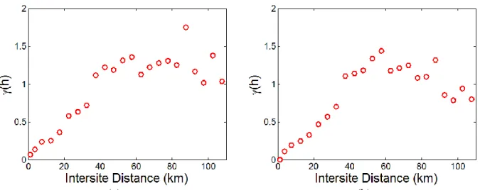
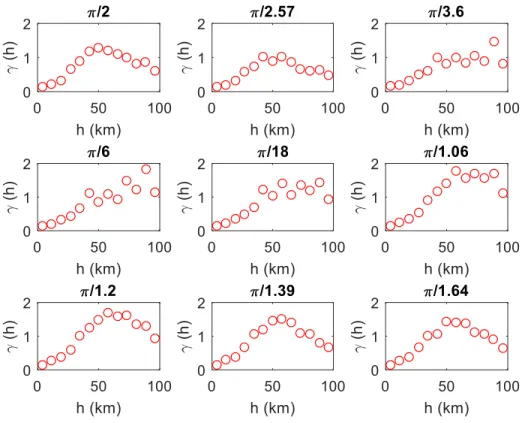
Figure 1.1 Proposed data-driven building seismic response prediction framework ... 4 Figure 3.1 Conceptual illustration of methodology used to develop inter-building interpolation model of peak structural responses ... 29 Figure 3.2 Locations of ground motion recording stations (red crosses) and epicenter (black dot) for the (a) 1994, Northridge; (b) 1999, Chi-Chi; (3) 2000, Tottori earthquake ... 31 Figure 3.3 Exponential trend line showing the relationship between the geometric mean PGA and rupture distance ... 32 Figure 3.4 Exponential trend lines showing the relationship between the (a) PSDR and (b) PFA for CMF-2 ... 35 Figure 3.5 Scatter plot showing the natural log of PSDRs for various site pairs with median inter-site distances of (a) 1.25 km, (b) 3.75 km, (c) 7.5 km and (d) 12.5 km for the CMF-2 structure subjected to the Northridge ground motions ... 37 Figure 3.6 Correlation coefficients for maximum (a) PSDRs and (b) PFAs versus the median inter-site distance for the CMF-2 structure subjected to the Northridge ground motions ... 39 Figure 3.7 Self-correlation coefficients for (a) PSDR and (b) PFA versus the median inter-site distance of all structures subjected to the Northridge ground motions ... 39 Figure 3.8 PSDR and PFA self-correlation coefficients versus the median inter-site distance for the (a) CMF-2 and (b) CMF-20 structures subjected to the Northridge ground motions ... 40 Figure 3.9 (a) PSDR and (b) PFA cross-correlation patterns for site-pairs with the CMF-2 and CMF-4 structures and (c) PSDR (d) PFA for site-pairs with the CMF-2 and CMF-20 structures all subjected to the Northridge ground motions ... 41 Figure 3.10 Correlation coefficients for (a) PSDRs and (b) PFAs versus the median inter-site

(11)

ix

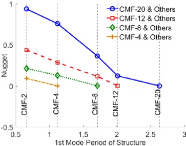
distance for CMF-2 paired with all other structures for the Northridge earthquake ... 43 Figure 3.11 Comparing CMF-2 self-correlation pattern for (a) PSDRs and (b) PFAs across the three events ... 44 Figure 3.12 Self semi-variogram for CMF-2 constructed using (a) classical and (b) Cressie and Hawkins estimator for the Northridge ground motions ... 47 Figure 3.13 Empirical and analytical self-semi-variogram for CMF-2 subjected to the Northridge ground motions ... 49 Figure 3.14 Self semi-variogram of PSDR for building CMF-2 with nine evenly distributed directions for the Northridge ground motions ... 50 Figure 3.15 Rose plot of self-semi-variogram for building CMF-2 using nine evenly distributed directions for the Northridge ground motions ... 50 Figure 3.16 Cross semi-variogram obtained from Northridge ground motions ... 52 Figure 3.17 Nugget effect of cross semi-variogram obtained from the Northridge ground motions ... 53 Figure 3.18 PSDR self-prediction result for the CMF-2 structure subjected to the Northridge ground motions ... 58 Figure 3.19 Bootstrap evaluation of (a) PSDR and (b) PFA self-prediction model for all structures ... 59 Figure 3.20 PSDR cross-prediction model performance (a) between CMF-20 and all other structures and (b) for all structure combinations (only median MARD) ... 60 Figure 3.21 Median MARD versus training dataset size ... 61 Figure 3.22 Comparing performance of cross-interpolation model between all structures for IM- and PSDR-basedsemi-variograms ... 62

(12)

x

Figure 3.23 Effect of response demand level on model performance for(a) PSDR and (b) PFA self-prediction for CMF-2 ... 63 Figure 3.24 Effect of number and spatial clustering of buildings on the performance of the interpolation model for the Northridge earthquake scenario ... 64 Figure 4.1 Multibuilding seismic response reconstruction framework ... 70 Figure 4.2 (a) Station map (red dots are stations; black star is epicenter) and (b) Response spectrum acceleration at 5% damping of all records for the Northridge earthquake ... 72 Figure 4.3 Overview of Perform3D model (a) TB-1 (b) TB-2 (c) TB-3 (d) TB-4 ... 76 Figure 4.4 (a) PSDR and (b) PFA distribution for TB-1 subjected to 152 ground motions from the Northridge earthquake ... 78 Figure 4.5 (a) PSDR and (b) PFA distribution for TB-2 subjected to 152 ground motions from the Northridge earthquake ... 78 Figure 4.6 (a) PSDR and (b) PFA distribution for TB-3 subjected to 152 ground motions from the Northridge earthquake ... 79 Figure 4.7 (a) PSDR and (b) PFA distribution for TB-4 subjected to 152 ground motions of Northridge earthquake ... 79 Figure 4.8 Plot showing (a) PSDR distribution (along height) and (b) mean PSDR (along height) versus the rupture distance for TB-1 ... 81 Figure 4.9 Trendlines for (a) mean PSDR and (b) mean PFA over height with respect to rupture distance ... 81 Figure 4.10 Visualization of Gaussian kernel ... 86 Figure 4.11 Example of randomly distributed building locations ... 93 Figure 4.12 PSDR prediction results for (a) TB-1 located at 33.790 N, 118.012 W and (b) TB-4

(13)

xi

located at 34.070 N, 118.150 W for the baseline scenario, cross-prediction case ... 95 Figure 4.13 PFA prediction results for (a) TB-1 located at 33.790 N, 118.012 W and (b) TB-4 located at 34.070 N, 118.150 W for the baseline scenario, cross-prediction case ... 95 Figure 4.14 MARD distribution for (a) PSDR and (b) PFA prediction for the baseline scenario 96 Figure 4.15 PSDR cross prediction result for baseline scenario using (a) KSVR and (b) KSVRW ... 98 Figure 4.16 PFA cross prediction result for baseline scenario using (a) KSVR and (b) KSVRW98 Figure 4.17 (a) Ranked PSDR prediction result for the baseline scenario and (b) effect of the training data percentage on model performance of the baseline scenario ... 99 Figure 4.18 PSDR prediction result for (a) randomized and (b) designated sensor locations .... 101 Figure 4.19 (a) PSDR distribution for TB-1 subjected to 40 near epicenter ground motions from the Northridge earthquake and (b) MARD distribution for PSDR cross-prediction based on high demand data subset ... 102 Figure 4.20 Effect of training data percentage on model performance for the high demand data subset scenario ... 103 Figure 5.1 (a) Location of epicenters and (b) histogram of magnitude of included earthquake events ... 112 Figure 5.2 (a) Locations and (b) histogram of number of stories of instrumented buildings ... 114 Figure 5.3 Example 13-story building sensor plan layout and accelerometer channel output subjected to the 2014 Encino earthquake... 116 Figure 5.4 (a) peak story drift ratio and (b) peak floor acceleration profile from the 1994 Northridge earthquake ... 117 Figure 5.5 Maximum response along building height of (a) peak story drift ratio and (b) peak floor

(14)

xii

acceleration from the 1994 Northridge earthquake ... 118 Figure 5.6 Peak floor acceleration trend over rupture distance of events with magnitude (a) less than 5 (b) between 5 and 6 (c) between 6 and 7 (d) greater than 7 ... 119 Figure 5.7 Colormap of V_S₃₀ database by Thompson et. al. [155] ... 122 Figure 5.8 Histogram of estimating distance between actual building site and the used estimated site ... 122 Figure 5.9 Flowchart for stage-1 regression iteration ... 125 Figure 5.10 Observed/Predicted ratio versus rupture distance of (a) PSDR and (b) PFA of Equation (5-5)... 128 Figure 5.11 Total residual versus (a) rupture distance, (b) building height, (c) magnitude and (d) ASCE-7 empirical period for PSDR of Equation (5-5) ... 129 Figure 5.12 Observed/predicted ratio versus rupture distance of (a) PSDR and (b) PFA of adopted generalized cross-building EDP reconstruction model in Equation (5-17) ... 131 Figure 5.13 Record residual



histogram of (a) PSDR and (b) PFA ... 132 Figure 5.14 (a) Correlogram of record residual from the adopted generalized cross-building EDP reconstruction model and (b) its fitted exponential semi-variogram model for PSDR and PFA of the 2007 Alum Rock earthquake... 136 Figure 5.15 (a) Record residual kriging interpolation result and observed/predicted ratio of PSDR using 30/70 percentage training testing split of recorded data from the 2007 Alum Rock earthquake ... 136 Figure 5.16 (a) Record residual kriging interpolation result and observed/predicted ratio of PSDR using 30/70 percentage training testing split of recorded data from the 1987 Whitter Narrows earthquake ... 136

(15)

xiii

Figure 5.17 Simulated coordinates for 2007 Alum Rock Area earthquake ... 137 Figure 5.18 Sites map of the 1994 Northridge earthquake ... 139 Figure 5.19 (a) PSDR and (b) PFA subjected to the 1994 Northridge earthquake from concrete moment frame model ... 140 Figure 5.20 Observed-to-prediction ratio versus rupture distance of (a) PSDR and (b) PFA from concrete moment frame models subjected to the 1994 Northridge earthquake ... 142 Figure 5.21 Total residual versus (a) rupture distance, (b) building height, (c) magnitude and (d) ASCE-7 empirical period for PSDR of the simulation dataset of the 1994 Northridge earthquake ... 143 Figure 6.1 Histograms of the (a) PSDR and (b) PFA total residual across all earthquake events ... 150 Figure 6.2 Histograms of PFA total residual of (a) the 1994 Northridge earthquake, (b) the 2014 South Napa earthquake, (c) the 1992 Landers earthquake and (d) the 2003 Big Bear City earthquake ... 151 Figure 6.3 Histograms of PSDR total residual of (a) the 1994 Northridge earthquake, (b) the 2014 South Napa earthquake, (c) the 1992 Landers earthquake and (d) the 2003 Big Bear earthquake ... 152 Figure 6.4 Proposed Bayesian hierarchical model layout ... 155 Figure 6.5 Q-Q plot for (a) PSDR and (b) PFA total residual of the 1994 Northridge earthquake ... 155 Figure 6.6 Simulation result of  and



2 of PSDR ... 161 Figure 6.7 Trend of the within-chain and the posterior marginal variance of  (var( | )



e ) from the Markov chain simulation of PSDR ... 161

(16)

xiv

Figure 6.8 Autocorrelation of  from the Markov chain simulation of PSDR ... 162 Figure 6.9 Trend of the Within-event residuals of all earthquakes from the Markov chain simulation of PSDR ... 162 Figure 6.10 Trend of the Within-event residuals of all earthquakes from the Markov chain simulation of PFA ... 163

(17)

xv

List of Tables

Table 3.1 Summary of historical earthquakes used to develop interpolation model ... 31

Table 3.2 Design information for concrete moment frame buildings ... 33

Table 3.3 EDP statistics of all five buildings for original intensity scenario, Northridge earthquake ... 34

Table 4.1 Summary of 1994 Northridge earthquake ... 72

Table 4.2 Summary of building characteristics ... 73

Table 4.3 Summary of building periods ... 76

Table 4.4 Summary of coefficients of variation (COV) along the building height ... 79

Table 4.5 Summary of F-scores ... 91

Table 5.1 Summary of included earthquake events ... 112

Table 5.2 Average median MSE of PFA interpolation ... 115

Table 5.3 Calibrated Model Parameter ... 126

Table 5.4 Calibrated Adopted Model Parameter ... 130

Table 5.5 Calibrated Adopted Model Parameter for Simulation Dataset of the Northridge earthquake ... 140

Table 6.1 Summary of Within-event residual of PSDR ... 165

(18)

xvi

Acknowledgement

The research presented in this dissertation is supported by National Science Foundation, Division of Civil, Mechanical and Manufacturing Innovation research grant number 1538866. Any opinions, findings, and conclusions or recommendations expressed in this dissertation are those of the authors and do not necessarily reflect the views of the sponsor.

I would like to thank my Ph.D. advisor, Dr. John W. Wallace for his continuous support and encouragement. I would also like to express my sincere gratitude to Dr. Henry V. Burton for his dedicated guidance and mentoring. Besides, I sincerely thank Dr. Jonathan P. Stewart and Dr. Arash A. Amini for their technical advices.

My special thanks to my parents for their unconditional support and sacrifices. I dedicate this dissertation to the memory of my grandmother Longxian Hu, who set a perfect example for me on honesty, bravery and diligence and is always in my heart. At last, I would like to acknowledge my wife, Xin Qian, for her professional suggestions and all the time we share from the very beginning.

(19)

xvii

VITA

2008-2012 B.Sc. in Civil Engineering, Hong Kong Polyethnic University, Hong Kong

2012-2014 M.Sc. in Civil Engineering, University of Michigan, Ann Arbor, MI

2014-2019 Ph.D. candidate in Civil Engineering, University of California, Los Angeles, CA

(20)

1

1. Introduction

1.1Overview

Earthquakes cause significant structural damage that can result in consequential economic loss due to operational downtime and monetary cost related to inspections and repair. In particular, in seismically active regions such as California, Japan, and New Zealand are facing critical challenges related to lower magnitude, more frequent earthquakes resulting in extensive efforts to complete post-earthquake inspection on large inventories of buildings. In addition, there is an increasing probability of high magnitude earthquake occurrences on active faults (e.g., San Andrews Fault, Puente Hills, etc.) that are likely to create significant challenges for the impacted areas related to post-earthquake inspections, repair and retrofit, and recovery as observed in Los Angeles, Taiwan and Mexico City [1–3].

Besides the time, effort, and expense of inspection, which is typically accomplished visually, building damage identification can also be achieved by Structural Health Monitoring (SHM). In specific, SHM involves remote sensing devices installed in the building to retrieve structural response histories (e.g., accelerations, displacements, strains) subjected to the seismic hazard (ground shaking), to determine Engineering Demand Parameters (EDP) such as peak floor acceleration and peak story drift ratio and use these data to identify and assess the importance of the damage. However, due to cost constraints related to installation and maintenance, SHM systems typically involve a relatively limited number of sensors in a limited number of buildings; to date, the vast majority of installations involve using accelerometers. Therefore, a major challenge associated with SHM systems involves data interpretation in buildings with sensors, as well as the lack of sensors in some buildings. An attractive option to address some of these issues involves reconstructing building seismic responses to gain additional value from SHM

(21)

2

installations, in both instrumented and non-instrumented buildings.

In addition to damage identification needs for seismic building responses subject to earthquake shaking, modern seismic risk assessment frameworks such as Performance-Based Earthquake Engineering (PBEE) developed by the Pacific Earthquake Engineering Research (PEER) Center [4–6] typically require conducting Nonlinear Response History Analysis (NRHA) to acquire EDPs from a suite of ground motions [7,8]. It is time consuming and computationally challenging to conduct such evaluations for complex structural systems, and an even more challenging to scale this effort up to a cluster of buildings or an inventory of buildings for a city or regional risk assessment [9,10]. Alternative approaches currently available within the earthquake engineering field to address these issues are to either estimate EDPs using site Intensity Measures (IM) such as Spectrum Acceleration (SA) instead of running NRHA simulations or to reduce model complexity. The former approach has been used since 1999 [11] as part of HAZUS estimation procedure [12] and applied in estimating earthquake losses [13–15]. The latter approach has been applied for regional seismic risk assessment studies (e.g., [16]).

An alternative approach is presented here to interpolate EDPs for a cluster of buildings at various scales using limited data sets from instrumented buildings. The framework presented aims to gain additional insight from instrumented buildings and also mitigate the computational effort of scenario-based risk assessment. To accomplish these goals, modern machine learning models are applied to predict seismic building responses at specified locations. The framework includes issues related to collecting and filtering data obtained from both simulation results and sensor recordings, scenario design, and model performance evaluation. Depending on the data available, a variety of scenarios are developed.

(22)

3

1.2Research Significance

The objective of the research reported is to develop a data-driven framework that predicts building seismic responses for a given building located at a given site using available recordings from co-regionally located buildings subjected to the same event, and recordings from actual buildings subjected to prior events. The goals of the research are to enable rapid 1) damage identification for individual buildings that are either instrumented or un-instrumented during a seismic hazard; 2) regional risk estimation for a given seismic event, and 3) risk assessment for a range of domains, including for individual buildings, limited (local) and large (city or regional) clusters of buildings, as well as various building types using models with various complexities. The data presented, mythologies applied, and evaluation approaches considered are used to demonstrate that the machine learning framework proposed provides valuable tools to address SHM and risk assessment challenges facing the earthquake engineering community.

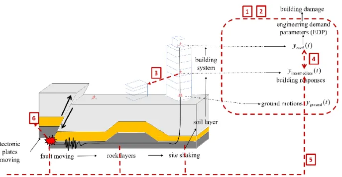
An illustration connecting the framework with a seismic event is provided in Figure 1.1. Earthquakes are caused by fault moving as a consequence of tectonic plates moving. The shaking generates seismic waves and travels through rock layers underneath the ground and soil layers. The shaking wave also travels upwards and is altered by soil layers and reaches the ground surface as is referred to as a ground motion response history, y_ground( )t , typically measured by accelerometers located on the ground surface. The shaking is further altered by the building system and produces seismic building response histories, y_roof( )t as measured at the roof level and

intermediate( )

y t as measured at intermediate levels. A number of buildings are instrumented with accelerometers at ground level and along the building height to record these building responses at seismic active regions provided by organizations such as United States Geological Survey and California Geological Survey. By retrieving these response data and converting them to EDPs,

(23)

4

building physical damage and its consequential monetary loss can be estimated. The core of this dissertation is to construct a framework that simulates the above-mentioned sophisticated scenario through data-driven means.

Figure 1.1 Proposed data-driven building seismic response prediction framework 1.3Outline of the Thesis

Seven chapters are used to present the proposed framework for building seismic response prediction. The red boxes with numbering on Figure 1.1 are covered in the referenced chapter to achieve the goal.

Chapter 1 provides the background and motivation for the research, as well as an outline of the dissertation (red box 1). A review of key literature most closely related to the proposed framework is presented in Chapter 2. Chapter 2 (red box 2) includes details to assess the viability of applying machine learning to solve earthquake engineering challenges by examining the nature of the existing problems, addressing important characteristics of machine learning algorithms, and

(24)

5

demonstrating applications using archived data. Chapter 3 (red box 3) presents an interbuilding interpolation scheme using Kriging to predict peak seismic response demands for a portfolio of reinforced concrete moment frame buildings subjected to a seismic event. Three historical scenario earthquakes (1994 Northridge, 1999 Chi-Chi and 2000 Tottori) are used to evaluate model performance. Chapter 4 (red box 4) expands the interpolation scheme by reconstructing EDP profiles of four representative tall buildings along building heights by utilizing two kernel-based machine learning methods, kernel ridge regression, and kernel support vector regression, respectively. A rigorous model evaluation technique, non-replacement bootstrap, is used to demonstrate the different approaches. Chapter 5 (red box 5) expands the previous two seismic demand reconstruction methodologies from scenario-based (subjected to a single event) to a generalized prediction model that incorporates event characteristics of structural and site dissimilarity with a mixed-effect statistical model. This approach is validated using data collected for California buildings between 1984 and 2018. Chapter 6 (red box 6) includes a discussion of several alternatives for event terms considered in the generalized prediction model including Bayesian and Frequentist approaches. Chapter 7 provides a summary and the primary conclusions.

(25)

6

2. A Critical Examination of the Viability of using ML to Address Structural

Engineering

2.1Introduction

The term Machine Learning (ML) is no foreigner to the structural engineering research community as pioneer applications, such as applying neural network [17,18] and regression analysis [19,20], can be tracked to early 1990s. Since ML methods at that time were often only treated as a method to maps nonlinear patterns, as discussed in [21], ML applications merely serves as an alternative to physics-based models. For instance, Ghaboussi, et. al. [17] developed a neural network mapping for experimental biaxial stress-strain relationship of concrete; however, the physics-based models of concrete were well-developed and it was much easier to interpret the data using physics-based models versus the ML model [17]. As early as 1997, Reich [22] provided a comprehensive review associated with the application of ML to solve civil engineering problems, from data collection, model creation, results evaluation using advanced ML techniques such as cross-validation and bootstrap. Due to computational speed and memory space issues, early ML models were restricted to solving classes of problems with limited data such that the prediction performance were merely comparable with physics-based models. Furthermore, ML models are typically considered to be black-box solutions that often lack the framework to gain physical insight.

Starting from late 2000s, driven by the decade long boost of development of Structural Health Monitoring (SHM) and rapid growth of computational power and data storage, the structural engineering community has gradually engaged in “big data” problems. The challenge to interpret large data sets collected through recordings from field monitoring and to extract information from data retrieved through numerous or complex computer simulations has brought

(26)

7

ML back to the front stage. Recent success stories for ML in many other fields and the growing number of ML application publications in structural engineering that have been initiated in recent years, has drawn more attention and interest to critically examine opportunities to use ML to solve structural engineering problems. Two major items have spurred this development. First, the amount and diversity of data have increased significantly. With the improvement in computational methods and structural modeling tools, many large complex structures can be analyzed by finite element method for multiple hazard levels or types. This significant increase in the problem scale and complexity can be challenging for physics-based models. On the other hand, ML methodologies have vastly improved with the state of art methods such as Convolutional Neural Network (CNN) [23,24], and feature fusion techniques [25–27] and these methods have been applied to solve structural engineering problems. With the increased data size and complexity, data-driven methods may be advantageous relative to traditional physical-based models in terms of capability and efficiency. For instance, the ability to assess structural performance for a regional and city scale models [27,28], as opposed to focusing on individual structural components and systems as has been common until recently, for multi-level hazard assessment for a range of intensities, is a case where ML is very attractive [8].

The modern ML applications in structural engineering field can be categorized into the following four general areas:

1. to predict structural nonlinear responses and damage;

2. to interpret experimental data and formulate empirical relations between structural properties and responses;

3. to retrieve information about structural characteristics through visual media; 4. to recognize patterns from SHM.

(27)

8

The objective of this chapter is to present ML methods and assess their ability to address current strucutral engineering challenges by examining the nature of existing problems, characteristics of ML methods, and current research directions. Specifically, challenges associated with collecting data, preparing sophisticated model simulations, and enhancing computation tools are reviewed. An introduction of ML is presented with brief descriptions of their mathematical formulations and capabilities. Following which, domain specific motivations to use ML methods in the structural engineering field are demonstrated with discussions on their corresponding challenges across the above mentioned four main perspectives, each supplemented with examples from recent research publications. Finally, future directions and opportunities to apply ML methods, including data source, model interpretability, and extrapolating ability are presented.

2.2Brief Introduction of Machine Learning 2.2.1General Formulation of ML Setting

Systematic approaches to create data-driven models appropriate to solve engineering problems have already been developed, i.e., surrogate modeling [29]. In the ML context, surrogate models can be treated as a subset of ML models that have a complex objective function to minimize

(i.e., non-convex function). Instead of directly solving the function, an alternative mechanism is

used to find a solution. For instance, the logit function converts the non-convex 0/1 loss of a

classification objective function into a logistic loss such that it can be solved through logistic

regression. To avoid confusion, this chapter will focus on the classic formulation of ML using a

universal language instead of discussing more broadly defined data-driven methods.

ML problems are typically categorized into two major tasks, supervised and unsupervised learning. The former is formulated using the ground truth, or the labeled data, i.e., actual damage classes of a pool of buildings, while the latter is not. Therefore, their applications are dependent

(28)

9

on the objective. Supervised learning can be further expanded into two sub-categories, (a) regression, where labeled data are continuous variables, and (b) classification, where labeled data are discrete class tags. Therefore, the goal of supervised learning is to generate a function that approximates the labeled data based on input observations. An unsupervised task, on the other hand, is to extract the inherent structure information from the given input observations, i.e., to search for clusters within the data.

For supervised learning, the dataset contains a collection of feature variables, a matrix X

with dimension n p , where n is the total number of observations (data points) and p is the number of features (independent variables); and a labeled response variable y , a vector of size

1

n representing labels of each observation. Similarly, a dataset for unsupervised learning includes a feature matrix X but not the response variable y. The objective of supervised learning is to solve the generalized optimization problem by minimizing an empirical risk defined in Equation (2-1) [27]. 1 1 arg min ( , ( ; )) ( ) n i i i y f x n 



₌   +   (2-1)

Where y_i is the response variable for observation i . f x( ; )_i  is the approximated response from the ML model based on the feature x_i and  represents the set of model parameters.  is a loss measure between the true value yi and the predicted value f x( ; )i  .  ( ) is a regularization term that adjusts model complexity by restricting the parameter set  through (.). The objective is to find the best set of model parameters, ˆ, that minimizes the empirical risk over training data with the regularization penalty considered. Equation (2-1) is a convenient generalized form and can be adopted by many supervised learning methods including ordinary least squares, ridge regression, LASSO regression, logistic regression, and kernel regression. Depending on

(29)

10

which ML method is adopted, the minimization problem can be solved with either a closed form solution, through gradient based methods, or convex approximation.

The objective function for unsupervised learning is shown in Equation (2-2), where  is the set of model parameters that characterizes a learning structure for the given dataset. The loss function  quantifies the costs to assign a data point x_i to a particular cluster. ML methods that can be generalized by Equation (2-2) include K-means and K Nearest Neighbors [30].

1 1 arg min ( ; ) n i i x n 



=   (2-2)

In statistical learning theory, the objective function expressed in Equations (2-1) and (2-2), is defined as an empirical risk over the training dataset, donated as I_n( )f for a given model f . The theoretical objective of ML problem is to minimize the expectation in Equation (2-3), which is an integration over entire data space. Limited by the amount of data sampled from the space, the ideal case is often approximated by minimizing the empirical risk of training data instead.

arg min ( ) ( , ( )) ( , ) X Y

I f y f x p x y dxdy

 =



  (2-3)

2.2.2Feature Engineering

Prior to training the model, applied ML methods always involve the process of selecting and extracting features which are found to influence model performance, improve training efficiency, and increase flexibility; all are necessary to tackle ML problems. A successful ML application usually deploys a standard algorithm; however, it also typically includes the ability to adjust features to achieve best possible prediction performance.

Feature selection can be categorized into three methods: filter, wrapper, and embedded. The filter method ranks original features according to an importance measure score such as scores from a Chi-square test or correlation coefficients between individual feature and response variable

(30)

11

and selects a subset of original features. The wrapper method involves recursively including or excluding features from current pool and selecting the best performing pool. Embedded methods are those ML algorithms which incorporate automatic feature selection, e.g., LASSO and ridge regression. Both filter and wrapper methods are good at avoiding overfitting issues by reducing model complexity and improving training efficiency by reducing duplicated features. Feature extraction consists of two major tasks that increase the effectiveness of ML models: 1) conducting dimension reduction over data through methods such as Principle Component Analysis (PCA), which performs linear mapping from the original data space to a lower dimensional space such that data variance over each orthogonal component is maximized; 2) transforming data into a higher dimensional space such that the patterns become sparse and separable, e.g., kernel-based ML algorithms [31].

Besides the general feature engineering techniques mentioned in the prior paragraph, specific feature designs have been proven to be very successful for domain-specific problems. For instance, the use of HAAR-like features achieved human-level accuracy with far less computational effort [32] for face recognition; SIFT [33] features are very effective for object detection within images, and the HOG [34] features are particularly good at human detection. However, these domain-specific feature engineering techniques require considerable trial and error testing and are designed to only work for very specific problems and data structures. Neural network approaches and the associated deep learning approaches are extremely popular in that they automate feature engineering to achieve state-of-the-art level performance in many pattern recognition and data mining domains. This approach has emerged due to the increase in computation power in recent years.

(31)

12

2.2.3Model Training and Performance Metrics

There are many well-established procedures for ML model training that attempt to achieve stable and effective prediction performance for new data (extrapolation) given a training dataset. One common strategy is k-fold cross validation (also discussed in [22]) that randomly splits a dataset into k different subsets and trains the model k times using the kth subset as testing data and the remaining k-1 subsets as training data. Among all k models, the best performing model over the testing dataset is selected. This procedure largely reduces overfitting on the training dataset. Another popular technique to avoid overfitting is Bootstrap, which randomly samples a subset of the data with replacement and trains the model M times. The final model is selected as an average over the predicted results (regression) or based on majority vote (classification) [35] from the M models. Both Bootstrap and k-fold cross validation effectively reduces model variances are unbiased and are the primary training techniques used in developing data-driven models presented in later chapters. These training procedures are evaluated by using various performance metrics for model selection. For example, performance metrics of binary classification models include accuracy, precision and recall [36] whereas performance metrics for multi-class classification models typically include using a confusion matrix and top-k class accuracy as shown in ImageNet [37] literature. Regression models are usually evaluated by Root Mean Squared Error, Median Absolute Error, and Median Absolute Relative Deviation as presented by Burton, Sun et. al. [27,28,38].

2.3Motivation of Using Machine Learning in Structural Engineering Field

For a long time, the structural engineering community has been developing models for real-world structures by conducting physics-based simulations and constructing prototypes to investigate uncertainties using laboratory tests. The traditional research path involves interpreting

(32)

13

results from the models and/or tests and combining observations (empirical and/or analytical) to develop guidelines, standards, or codes of practice for structural design, construction and retrofit. The approaches involved range from statistical curve fitting to physics-based analytics using computer simulations. Classic examples include the steel moment connection and steel shea wall system development by Qian and Astaneh-Asl [39,40] and a structural wall and coupling beam development by Wallace [41]. This common research path usually includes considerable engineering judgement and commonly requires some level of consensus to become standard practice. Limitations of this approach are apparent, such as the lack sufficient model complexity to accurately represent the dataset which leads to empirical approximations and, sometimes, cumbersome rules and step functions where small changes in design variables lead to undesirable outcomes. In addition, these approaches often include relatively crude factors (e.g., load and capacity-reduction) to account for uncertainties in the confidence intervals based on incomplete information.

Due to the rapid improvement in computational resources (speed, memory, storage, visualization), current mechanics-based analyses, such as finite element analysis using OpenSees [42] and Perform3D [43], are capable of simulating complicated structure systems from relatively simple nonlinear behavior subjected to loadings from multiple hazard types (earthquakes, hurricanes) at various load intensities [44,45]; these analyses tend to generate a lot of structural response simulation data. A study by Burton et. al. [46], where building seismic performance was assessed for a set of archetypical structural models representing existing wood frame buildings in Los Angeles using four different retrofitting schemes with thousands of Nonlinear Response History Analyses (NL-RHA). In addition, evaluation of structural safety has expanded from collapse prevention of single buildings to more diverse and comprehensive studies that involve

(33)

14

assessment of a spectrum of damage states for a range of structure system types, which then enables multi-variable risk assessment studies using tools such as HAZUS [11,12,47]. Guan et. al. [48] performed intensive Incremental Dynamic Analysis (IDA) to assess the seismic performance of an innovative self-centering steel moment frame and to assess economic risk using the FEMA P-58 procedure [49]. In addition to evaluating individual structures, the risk assessment could also be applied across the regional geo-spatial dimension by analyzing structural responses at the portfolio scale level. Regional loss assessment is demonstrated by DeBock et. al. in [14] and Sun et. al. [28], where a set of concrete moment frame buildings are subjected to an actual earthquake scenario at a number of sites distributed over an urban region. It is shown that the current structural research in hazard mitigation is moving towards to more sophisticated hazard scenarios that generate extreme volumes of data, which are not suitable for some of the traditional approaches that are less capable or less efficient at extracting information from the multiple dimensional data space.

With the continuing growth of experimental data accumulated in the structural engineering field and the use of more advanced technologies to capture additional data and data types from experiments (i.e., digital image technique to capture stress distribution on concrete slender wall [50]), traditional data interpolation techniques are insufficient to explore and identify data patterns for a broad range of structural parameters among a large set of experiment events. A recent database developed by Abdullah and Wallace [51] collects detailed, organized, and parameterized information from more than 1000 reinforced concrete wall tests available in the literature, which is the largest of its kind. Traditional statistical tools are not ideal to examine data trends in such a large dataset. On the other hand, modern ML techniques have advantages, such as reduced influence of outliers, expanded dimensional parameter spaces (higher model complexity), and

(34)

15 improved predictions.

Another emerging trend is the development and expansion of SHM over the last several decades to the point where rapid assessment based on measured data can provide valuable decision variables. The concept of SHM is to remotely monitor the status (e.g., level of damage) within a structure using advanced sensing technologies based on data collected during an event. The process involves data cleaning, feature selection, and statistical model development for damage detection, all of which can be achieved using modern ML algorithms. As early as 2006, Farrar and Worden discussed some of the challenges facing by SHM, such as over-prediction of damage, which is an application of statistical pattern recognition. They noted that key challenges include structural damage is often localized whereas monitoring is often accomplished using global measurements, where it is difficult to identify what has influenced the minor changes in the system responses (lack of uniqueness, in space and time), especially given the relatively sparse data measurements that were common at the time. With more computation power and with state-of-the-art ML models, these challenges are being overcome. For example, the use of kernels to extract key features from both space and time domain and develop a discriminant model for damage detection by Santos et. al. [26], incorporation of state-of-the-art deep learning CNN models to make use of image data [52], the application of random forest, an advanced decision tree algorithm, for assessing post-earthquake structural safety of buildings [8].

The National Hazards Engineering Research Infrastructure (NHERI) is a platform that provides a network of research laboratories located at universities around the country that conducts experiments and collects experimental data in various forms related to hazards such as images of observed physical damage (photos, video) and measured data from a wide-range of sensor types from tests conducted in that involve water systems, energy and communication systems,

(35)

16

residential , commercial, and industrial buildings, other infrastructure (dams, bridges, roads, tunnels). This broad range of applications provides a tremendous opportunity for the structural engineering community to search for data-driven approaches to help address some most challenging problems in our field.

The preceding discussion provided a general overview of use of modern ML algorithms, and the opportunities to expand the use of structural response history data obtained from sensors, images to identify structural and non-structural damage, and of ML models. Four critical aspects associated with these challenges are discussed in the following sections.

2.4Examples of Machine Learning Applications in structural engineering

A board range of relatively recent ML publications in structural engineering field are summarized based on their application into the four major categories: 1) predicting nonlinear structural responses and damage; 2) experimental data interpretation and empirical fitting; 3) information extraction from visual media; and 4) pattern recognition for structural health monitoring.

2.4.1Predicting Structural Nonlinear Responses and Damage

The ability to use ML to predict using either regression or supervised learning provides a data-driven alternative to determine structural responses or classify damage states for structures under various scenarios. Structural demand data usually comes from a large set of NL-RHA, although it is becoming more common that such data might be retrieved from instrumented buildings. Depending on the objective, these NL-RHA were conducted using models ranging from 1) a single type of structure whose structural characteristics may vary; 2) a single or pool of structure models subjected to a defined hazard at different intensity levels; and 3) a cluster of structure models in a regional assessment scenario.

(36)

17

To detect structural damage, Zhang et. al. [8] applied random forest for damage detection for a 4-story reinforced concrete building case study using the response demand output from NL-RHA, whereas Bagriacik et. al. [53] applied logistic regression, boosting regression trees and random forest to identify individual structural pipe damage status. To predict structural seismic responses using regression algorithms for a single structure, example applications include [54], where Support Vector Regression (SVR) was used to predict seismic engineering demand parameters using NL-RHA data from a single degree of freedom system, a four-story building and a bridge pile, whereas Soleimani et. al. [55] applied LASSO regression to determine uncertain parameter significance seismic demand prediction for an irregular bridge. To estimate demand parameters that are critically related to structural damage, Burton et. al. proposed a framework for aftershock collapse vulnerability using mainshock intensity, structural responses, and physical damage indicators [38], whereas Mangalathu, et. al. estimated seismic vulnerability and fragility curves for skewed bridges [56].

For a regional setting, Sun et. al. [28] reconstructed peak structural response engineering demand parameters by utilizing structural and spatial dissimilarities within in a seismic event using kriging models, and further extended the framework using kernel-based ML regression algorithms, kernel ridge regression, and kernel SVR to reconstruct a profile of responses for engineering demand parameters [27]. Burton et. al. [10] presents a conceptual framework for modeling post-earthquake housing recovery with building-level damage limit states which could be scaled up to an event scenario at the region level.

2.4.2Experimental Data Interpretation and Empirical Fitting

One advantage of adopting modern ML algorithms is that it is possible to extract data patterns from complex structural system behavior and identify structure damage without human

(37)

18

inspection, which is the most common approach used. Ghiasi et. al. [25] conducted an experiment on a four-story prototype structure and mimicked damage scenarios by removing braces at each floor. A SVM classifier with a combined parameter kernel function was applied to predict structural damage scenarios using acceleration sensor response history signals at each floor as input features.

Besides the complex tasks of damage detection mentioned above, which is not viable through traditional empirical data fitting in a laboratory testing, ML also shows superior prediction performance on traditional tasks. For example, Vu and Hoang [57] proposed a kernel-based SVM model to map factors that influenced the punching shear capacity of fiber-reinforced polymer (FRP) from a dataset of laboratory tests performed on FRP-reinforced concrete slabs and demonstrated that the approach outperformed traditional formula-based methods based on RMSE. Naeej et. al. [58] applied a simple ML algorithm, decision tree, to predict lateral confinement coefficients in reinforced concrete columns to show that the approach outperformed traditional empirical formula. These two examples, one that deploys relatively complex SVM algorithm, and one that uses a simple decision tree, both demonstrate that ML algorithms can provide more accurate information than traditional empirical formulas to fit patterns for large datasets.

2.4.3Information Extraction from Visual Media

Traditionally, structural damage detection at the structural component level through visual media has been accomplished by converting image data into strain distribution data using Digital Image Correlation (DIC), a mechanism based on a technique that captures local deformations using cross-correlation between randomly painted dots on a concrete surface, such as [59], [60] and [61]. The limitation is clear: 1) DIC requires a randomly painted dot field over the surface of interest, which is, for the most part, only practicable in laboratory setup; 2) a consistent length of image

(38)

19

sequence is necessary for calculating cross-correlations between painted dots; and 3) the converted damage indication data, the local strain distributions, only accounts for a subset of the information available from an image.

Vision-based techniques can extract additional information from image data. For example, Yeum and Dyke [62] deployed HOG and HAAR feature-based object detection schemes with a sliding window search to identify cracks near bolts from structure images. The HOG [34] and HAAR feature [32] classifiers are mainly texture feature extractors and are generally not as successful at image feature extraction as the CNN technique, which is extremely efficient in extracting both marco- and micro-scale features from images. It is superior in terms of unrestrained image input, accessibility and fast inference speed compared to traditional image processing techniques. Due to the flexibility of CNN for supervised learning problems, it has been deployed quite extensively to solve vision-based automatic damage detection problems. Cha et. al. [24,63] applied a region-based deep learning scheme to detect different damage types and concrete cracks in images of structures. Kong and Li [64] applied CNN to detect crack opening in steel bridge components under repetitive loadings from video clips. Other applications for damage detection using images include [65–68].

2.4.4Pattern Recognition for Structural Health Monitoring

Pattern recognition is an essential part of SHM in order to evaluate the tremendous amount data collected from various sources and to monitor structural condition to enable assessment in a timely manner. One major challenge noted in the literature is the ability to identify critical features that are associated with structure damage. Traditional ways include wavelet transformation and Fast Fourier Transform (FFT) which are limited because these methods are highly sensitivity to outliers. Data-driven approaches using ML are found to be more robust in dealing with complex

(39)

20

structure systems and various sources of input signals [69]. According to Worden and Manson [70], there are four levels of application for the data-driven approaches in SHM to: 1) detect if damage exists in the structure; 2) extract the probable location of the damage; 3) estimate the extent of the damage, and 4) infer information regarding the safety of structure. ML classification algorithms are suitable for level 1 e.g., [25,26,71], which adopt supervised ML algorithms for damage detection. While [72] applied an unsupervised, nonlinear principle component learning algorithm analysis together with auto-associative neural network to select features to predict stiffness changes from a synthetic bridge model (level 3). Another example of feature extraction using ML is by Rafiei and Adeli [73] where restricted Boltzmann machine was applied for damage related feature extraction followed with a classification neural network to detect damage in a 38-story reinforced concrete building.

ML algorithms may provide superior performance for these damage-related feature extraction examples compared to traditional physics-based methods given its capability in pattern recognition [73,74].

2.5Discussion in Applying Machine Learning to Structural Engineering

Previous discussions cover a wide range of ML applications at four major fronts of strucutral engineering community:

1. To predict structural responses and damage for stochastic excitation, such as seismic and wind loading, or stochastic structural characteristics;

2. To interpret experimental data where the test setting and scenarios are complex such that physics-based models either perform poorly or are limited to a particular configuration or problem type (versatility);

(40)

21

4. To recognize patterns from SHM data to inform structural system status.

In this section, we intend to critically discuss three domain challenges that we are facd in utilizing ML in structural engineering, data source, model interpretability and extrapolation fidelity.

2.5.1Data Source

One big contributor of the success of ML is the access to more data. Although the amount of data required to achieve ideal performance for ML models depends on the problem scenario and goal, it is essential to have sufficient data that the sampled group could represent the true distribution. Traditional data from structural engineering is often limited in its quantity and diversity, e.g., NL-RHA structural responses from a particular building model, cyclic behavior of a specific structural component. In these cases, it is not ideal to employ ML to capture the entire physical phenomenon behind finite element simulation or laboratory testing. On the other hand, there are ML applications that utilize more diverse structural response data across spatial domain such as [27], which, however; does not cover a diverse range of structural dissimilarities. The challenge is to collect a subset of data from the true data distribution that is representative in diversity and quantity such that ML algorithms are able to discover the underlying patterns of structural system within the domain objective. The shortage of data can be compensated for by incorporating domain knowledge within the ML model such that additional domain knowledge is introduced to reduce the complexity of the model space and consequently reduce necessary amount of data to fit the ML model. In addition, some statistical procedures may also aid through data augmentation, e.g., Monte Carlo simulation, to generate synthetic data. Future efforts are likely to examine both options, i.e., collecting more diverse real and synthetic data and incorporating domain knowledge for model design.

(41)

22

However, the impact of outlier data might be more critical to certain ML algorithms, suc as logistic regression, due to their low robustness to noise. There are anomaly detection procedures for ML, such as using clustering techniques (DBSCAN [75], K-means [76]) and Z-score [77]; however, it also is necessary to include structural engineering domain-specific outlier detection procedures in ML applications. Ideally, the data-driven anomaly detection should be merged into physics-based outlier detection. In other words, the universal data filtering procedure of ML models should be modified with structural engineering domain knowledge, which has not been demonstrated in most recent research works.

2.5.2Model Interpretability

One of the most significant challenges associated with a ML model is interpreting the physics meaning of the model parameters. A commonly held view is that a ML model is a black box, i.e., there are no physical bounds that can be derived from a data-driven model. One option to address this issue is to deploy ML evaluation procedures (e.g., k-fold cross validation) over traditional statistical learning models to enable some degree of interpretability [28]. In addition, some recent efforts have demonstrated the potential of introducing domain knowledge into ML algorithms by incorporating a physics-based loss function, e.g., to embed hard conditions with a langrage multiplier into the loss function [78,79]. This approach provides a means to explain some of the ML model by adding a physics-based law into the objective function (Equation (2-1) and (2-2)). In [80], a spectrum of approaches are discussed that leverage the wealth of domain knowledge to improve performance data-driven models by adding domain knowledge, such as including theory guided model design or learning and regularization. However, combining ML and physics-based models remains a challenging problem that will be explored with future research.

(42)

23

2.5.3Model Extrapolation Ability

The ability to extrapolate the results of a ML model is another challenge and is also referred to as overfitting. Standard ML procedures involve data-based extrapolation by using training/testing split, k-fold cross validation, bagging and bootstrap, as well as other means. In addition, random forest provides a robust method to avoid overfitting given its stochastic procedure in generating trees in both feature and data space. For structural engineering, it is important to identity and apply domain knowledge to help avoid overfitting issues. The combination of a data-driven procedure and domain knowledge, similar to dealing with data sparsity, may provide a powerful combination. Although extrapolation has been extensively studied in the ML field, it could be more critical in applications of the strucutral engineering field given the high sensitivity of some strucutral responses. For example, to simulate a regular 40-story tall building, thousands of parameters are needed for configuration such as strucutral component geometry dimensions, material properties, external loadings, and construction conditions such that complex ML is almost unavoidable. Consequently, complex ML models require large amounts of data, better noise filtering processes, and careful model tuning to reduce the effects of overfitting.

2.6Summary

In this chapter, application of ML within civil engineering since the early 1990s, when the approach was introduced, are reviewed. ML applications in structural engineering field were initially motivated as an alternative to physics-based modeling to map nonlinear experimental data, later deployed for damage detection as a data-driven pattern recognition tool in SHM, and recently expanded to multiple fronts due to the large volume of data now available in structural engineering problems and the rapid growth of computational power, which consistently affect the viability to apply ML to solve strucutral engineering challenges.

(43)

24

As the strucutral engineering community has considered various approaches to developing ML models, ML models were discussed earlier this chapter using a universal setting related to model formulation, feature engineering, model training, and performance-driven tuning. This brief discussion summarizes current knowledge related to ML and identifies the complimentary steps required to develop a ML model. In addition, the various ML algorithms are grouped under the empirical risk objective from learning theory to regularize them into optimization formulations. This discussion is provided to help establish a consistent scenario setting or utilization of ML.

Subsequently, the motivations behind the interest in applying ML to strucutral engineering research and example applications from the literature were organized into four major categories: 1) strucutral response regression and damage classification; 2) experimental data fitting; 3) information extraction from visual data, and 4) pattern recognition in monitoring data. The literature provides various examples on the application of ML and demonstrates its potential; however, these examples share a common impression that the adoption of ML in structural engineering is still at early stage and the lacks approaches for comprehensive performance evaluation and universal model development procedure. Therefore, with regard to the above mentioned four categories, a detailed discussion is included on potential future directions for ML in three critical areas, namely: data source, model interpretability, and extrapolation ability. Data source is the primary concern when developing and applying data-driven models. The degree of to which the data represent the true distribution is directly related to resulting model capabilities, which can be improved by increasing the diversity and fidelity of the training data. Another critical concern is associated with the ability to interpret of ML models, which is, in-part, a challenge within our community due to lack of knowledge of ongoing developments within the data-driven field. Some recent research has indicated that progress is being made in this area and that ML

(44)

25

offers opportunities to develop models with domain-localization in structural engineering. The last topic is related to the ability to extrapolate the results of a ML model and problems associated with overfitting. Various of ML techniques are proven to be very effective against overfitting; however, it remains as a challenge to adopt these techniques for strucutral engineering problems. It should be noted that these three challenges are not independent. For example, the overfitting issue could be addressed by increasing data diversity and is therefore connected to data source. Making use of domain knowledge could potentially help with the ability to interpret model results and also reduce the amount of data needed.

To summarize, there are a vast number of opportunities within strucutral engineering research to address current challenges with data-driven ML models. However, challenges to develop such models exist such as data source, model interpretability and extrapolation. Creating ML models specific for strucutral engineering may be one future direction.

(45)

26

3. Inter-Building Interpolation of Peak Seismic Response using Spatially

Correlated Demand Parameters

3.1Introduction

During the period following a major earthquake, building owners, users and local and state officials are tasked with deciding whether damaged buildings can be re-occupied and reused. This decision can be informed by different types of post-event condition assessments. Seismic instrumentation and monitoring are one tool that is used to provide rapid damage detection and inform system-level evaluations. Accelerometers are placed in carefully chosen locations in plan and along the height of the building. Translational floor accelerations recorded during earthquakes are then used to compute velocity, displacement and story drift demands [81]. Using these recorded and computed response demands, a rapid diagnosis can be performed using one of several alternative damage measurement techniques. Response measurements from instrumented buildings can also be used to conduct real-time assessment of earthquake-induced damage, economic losses and social impacts [82].

Numerous studies have developed tools and techniques for interpolating structural response demands measured through seismic instrumentation, along the height of a building, i.e. intra-building response interpolation [83,84]. However, no research is available that has explored the possibility of inferring structural demands in non-instrumented buildings using response measurements from instrumented buildings, i.e. inter-building interpolation. With the decreasing costs of remote sensing technologies [85,86], seismic instrumentation of new buildings is becoming increasingly popular [87,88]. The city of Los Angeles, which has the only mandatory seismic instrumentation program in a US city, requires accelerometers be installed at the base, mid-level, and roof to obtain a permit for all buildings over ten stories as well as for buildings over