Polygonal Spatial Clustering

(1)

DigitalCommons@University of Nebraska - Lincoln

Computer Science and Engineering: Theses,

Dissertations, and Student Research Computer Science and Engineering, Department of

4-2011

Polygonal Spatial Clustering

Deepti Joshi

University of Nebraska-Lincoln, [email protected]

Follow this and additional works at: https://digitalcommons.unl.edu/computerscidiss

Part of the Computer Sciences Commons, and the Other Computer Engineering Commons

Joshi, Deepti, "Polygonal Spatial Clustering" (2011). Computer Science and Engineering: Theses, Dissertations, and Student Research. 16.

https://digitalcommons.unl.edu/computerscidiss/16

This Article is brought to you for free and open access by the Computer Science and Engineering, Department of at DigitalCommons@University of Nebraska - Lincoln. It has been accepted for inclusion in Computer Science and Engineering: Theses, Dissertations, and Student Research by an authorized administrator of

(2)

POLYGONAL SPATIAL CLUSTERING

by Deepti Joshi

A DISSERTATION

Presented to the Faculty of

The Graduate College at the University of Nebraska In Partial Fulfillment of Requirements For the Degree of Doctor of Philosophy

Major: Computer Science

Under the Supervision of Professors Ashok Samal and Leen-Kiat Soh

Lincoln, Nebraska

(3)

POLYGONAL SPATIAL CLUSTERING

Deepti Joshi, Ph.D.

University of Nebraska, 2011

Adviser: Ashok Samal and Leen-Kiat Soh

Clustering, the process of grouping together similar objects, is a fundamental task in data mining to help perform knowledge discovery in large datasets. With the growing number of sen-sor networks, geospatial satellites, global positioning devices, and human networks tremendous amounts of spatio-temporal data that measure the state of the planet Earth are being collected every day. This large amount of spatio-temporal data has increased the need for efficient spatial data mining techniques. Furthermore, most of the anthropogenic objects in space are represented using polygons, for example – counties, census tracts, and watersheds. Therefore, it is important to develop data mining techniques specifically addressed to mining polygonal data. In this re-search we focus on clustering geospatial polygons with fixed space and time coordinates.

Polygonal datasets are more complex than point datasets because polygons have topolog-ical and directional properties that are not relevant to points, thus rendering most state-of-the-art point-based clustering techniques not readily applicable. We have addressed four important sub-problems in polygonal clustering. (1) We have developed a dissimilarity function that integrates both non-spatial attributes and spatial structure and context of the polygons. (2) We have ex-tended DBSCAN, the state-of-the-art density based clustering algorithm for point datasets, to po-lygonal datasets and further extended it to handle popo-lygonal obstacles. (3) We have designed a suite of algorithms that incorporate user-defined constraints in the clustering process. (4) We have

(4)

developed a spatio-temporal polygonal clustering algorithm that uniquely treats both space and time as first-class citizens, and developed an algorithm to analyze the movement patterns in the spatio-temporal polygonal clusters. In order to evaluate our algorithms we applied our algorithms on real-life datasets from several diverse domains to solve practical problems such as congres-sional redistricting, spatial epidemiology, crime mapping, and drought analysis. The results show that our algorithms are effective in finding spatially compact and conceptually coherent clusters.

(5)

ACKNOWLEDGEMENT

I would like to thank my advisors Dr. Ashok Samal and Dr. Leen-Kiat Soh for their con-tinuous guidance and support throughout the course of my doctoral studies. They have helped me become the scholar that I am today. Without their patience and faith in me, I wouldn‘t have ac-complished the goal of finishing this dissertation. I am also thankful for the guidance of my su-pervisory committee members: Dr. Peter Revesz, Dr. David Marx, and Dr. Xun-Hong Chen. I would like to thank the Department of Computer Science and Engineering at the University of Nebraska-Lincoln for providing me this great opportunity. Finally, I would like to thank my fami-ly, especially my parents Mr. Ravinder Joshi and Mrs. Neelum Joshi, and my husband Mr. Arpit Sharma for their continuous love and support.

I am also grateful to the National Science Foundation for funding my research. This dis-sertation is based upon work supported by the National Science Foundation under Grants No. 0219970 and 0535255.

(6)

List of Tables

Table 1:Different characteristics of spatial object attributes ... 24

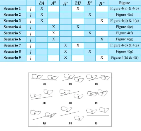
Table 2: Different possible scenarios based on topological relationship of a linear feature (l) with two polygons (A and B) ... 26

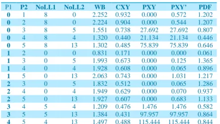
Table 3: Statistics and the distances between polygons using different distance functions (WB Distance, CXY Distance, PXY Distance, PXY‘ Distance and PDF). ... 32

Table 4: Ranking of pair-wise distances between polygons ... 33

Table 5: Ranking of selected pair-wise distances between polygons ... 34

Table 6: Attributes for Watersheds ... 38

Table 7: Clustering results for Watershed Dataset ... 40

Table 8: Gap Statistic results for the watershed dataset ... 41

Table 9: Attributes for Counties polygons ... 42

Table 10: Clustering results for County Dataset ... 45

Table 11: Gap Statistic results for the county dataset ... 45

Table 12: Comparison of clustering results for Nebraska Dataset ... 129

Table 13: Comparison of clustering results for Nebraska Dataset (Contd.) ... 129

Table 14: Comparison of clustering results for Indiana Dataset ... 130

Table 15: Comparison of clustering results for Indiana Dataset (Contd.) ... 130

Table 16: Runtime Comparison (Minutes) on Intel Pentium processor T4300, 4GB memory ... 131

Table 17: School districts result statistics ... 134

Table 18: Assault clusters discovered by STPC using different parameter values ... 166

Table 19: Change statistics along with the movement code for selected assault spatio-temporal clusters. ... 188

Table 20: Co-occurrence Matrix showing the Eight Movements that occur together for the California drought dataset from Jan 2000 to May 2010. ... 190

(10)

List of Figures

Figure 1: Separation distance where the transitive relation does not hold. ... 14

Figure 2: Minimum and maximum distance between vertices. ... 14

Figure 3: Comparison of Hausdorff distance with centroid distance. ... 15

Figure 4: Topological relationship between two polygons based on a linear feature – linear feature may intersect the interior, exterior or the boundary of a polygon. ... 26

Figure 5: A set of census blocks in Lincoln, NE and the locations of the sites for liquor licenses.

... 31

Figure 6: Subset Sample Dataset 2, along with the pair-wise distances between the various polygons. ... 35

Figure 7: (a) Polygons (subset of watersheds in Nebraska) used to form a cluster (b) Polygons along with linear spatial objects. ... 36

Figure 8: (a) Polygons (subset of watersheds in Nebraska) used to form a cluster (b) Polygons along with areal spatial objects. ... 37

Figure 9: Dataset for the first experiment – Watersheds in the state of Nebraska along with selected streams and lakes used as spatial objects ... 38

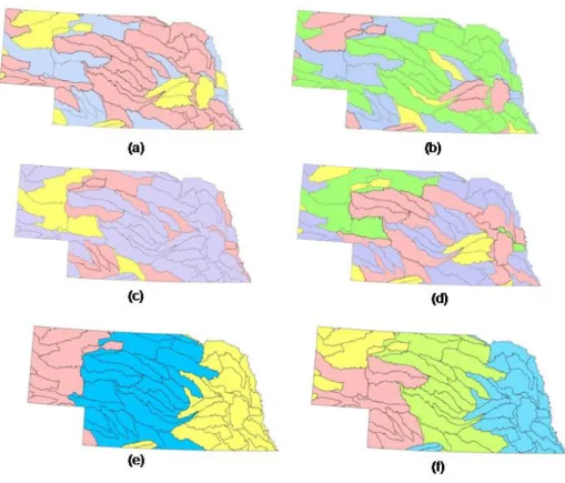
Figure 10: Result of clustering watersheds with. k = 3 ((a),(c),(e)) and k = 4((b),(d),(f)) using different combinations of non-spatial, structural and organizational attributes. ... 40

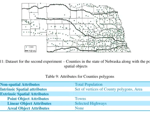
Figure 11: Dataset for the second experiment – Counties in the state of Nebraska along with the point and linear spatial objects ... 42

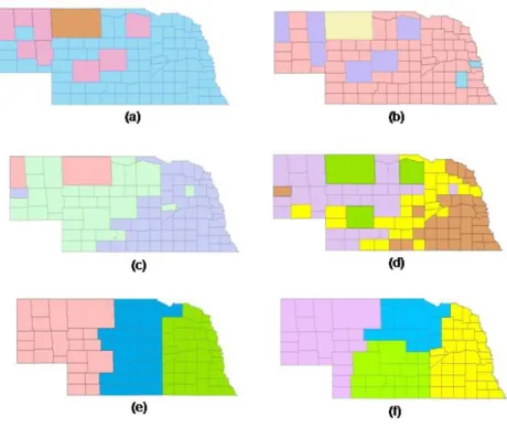
Figure 12: Result of clustering counties with. k = 3 and k = 4 using different combinations of non-spatial, structural and organizational attributes. ... 45

Figure 13: Radial spatial partitions of a polygon‘s neighborhood. Note that here the first sector is as shown, and the ordering is clockwise. This is arbitrary for illustration purpose. ... 54

Figure 14: Synthetic set of polygons (Red – Core Polygon, Green - -neighborhood of the core polygons) ... 55

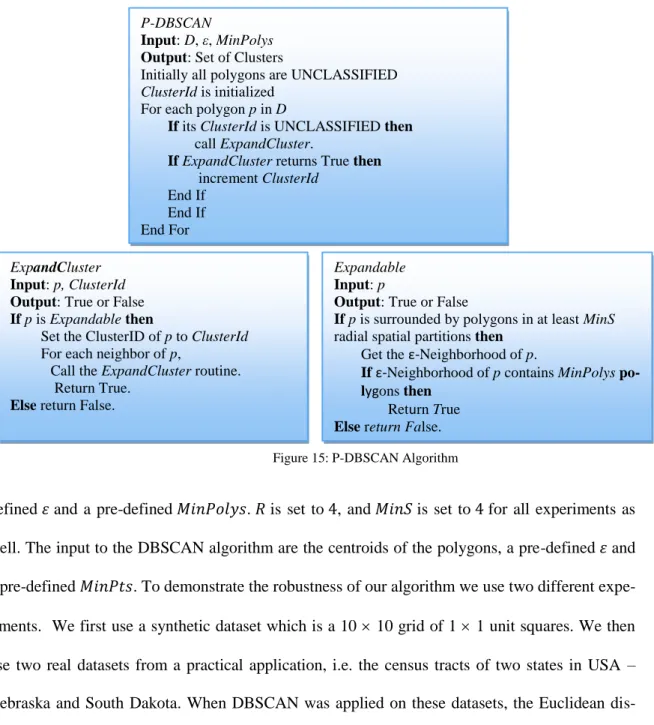
Figure 15: P-DBSCAN Algorithm ... 58

Figure 16: Result of clustering using DBSCAN (a) Polygons used for clustering (b) Expanded version of dataset showing ... 59

Figure 17: Result of clustering using DBSCAN (a) (b) First core

polygon(Red) and its - neighborhood (Green) (c) Consecutive core polygon detected and its -neighborhood (d) Further progression of core polygon detection belonging to the same cluster (e) Final result – All polygons belong to the same cluster. ... 59

Figure 18: Result of clustering using P-DBSCAN (a) Polygons used for clustering (b) First core polygon(Red) and its -neighborhood

(11)

(Green) (c) Further progression of core polygon detection belonging to the same

cluster (d) Final result – All polygons belong to the same cluster ... 60

Figure 19: Census Tract Polygons in Nebraska dataset ... 61

Figure 20: Results of clustering using DBSCAN (a) (b) (c) (d) ... 61

Figure 21: Results of clustering using P-DBSCAN (a) (b) (c) (d) (e) (f) ... 62

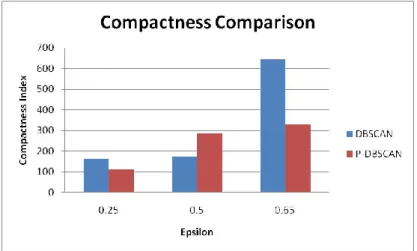
Figure 22: Compactness Ratio for clusters formed using DBSCAN and P-DBSCAN ... 62

Figure 23: Census Tract Polygons in South Dakota dataset ... 63

Figure 24: Result of clustering using DBSCAN (a) (b) (d) ... 63

Figure 25: Results of clustering using P-DBSCAN (a) (b) (c) (d) ... 64

Figure 26: Compactness Ratio for clusters formed using DBSCAN and P-DBSCAN. ... 65

Figure 27: Radial spatial partitions of a polygon‘s neighborhood. Note that here the first sector is as shown, and the ordering is clockwise. This is arbitrary for illustration purpose. ... 75

Figure 28: Synthetic set of polygons (Red – Core Polygon, Green - -neighborhood of the core polygons) ... 76

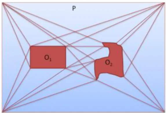
Figure 29: Sample visibility graph for a single polygon. O1 and O2 are obstacles while the lines constitute the visibility graph. ... 78

Figure 30: Sample visibility graph for a set of polygons in the presence of obstacles. The purple-outlined rectangles are polygons, the red polygons are obstacles with yellow-highlighted zones of influence, and the blue lines constitute the visibility graph. ... 79

Figure 31: Polygons A & B are completely visible to each other ... 80

Figure 32: Polygon A and Polygon B are partially visible to each other under Type A partial visibility ... 81

Figure 33: Polygon A and Polygon B are partially visible to each other under Type B partial visibility ... 81

Figure 34: Polygon A and Polygon B are invisible to each other ... 81

Figure 35: Pre-PDBSCAN+ algorithm. ... 86

Figure 36: P-DBSCAN+ clustering algorithm. ... 86

Figure 37: (a) Lincoln, NE census tracts – 55 polygons with 1211 vertices. (b) Simplified Lincoln, NE census tracts using the Douglas-Peucker algorithm – 55 polygons with 408 vertices. ... 88

(12)

Figure 39: Result of clustering using P-DBSCAN, i.e. without taking the obstacles into

consideration  = 200 ... 90

Figure 40: Result of clustering using DBCLuC with  = 200. ... 90

Figure 41: Result of clustering using P-DBSCAN+ with  = 200 and.  = 1.0 ... 90

Figure 42: Result of clustering using P-DBSCAN++ with  = 200 and  = 1.0, 0.5 ... 91

Figure 43: Census tract dataset of the city of Lincoln, NE with 55 polygons and 3 obstacles. ... 91

Figure 44: Census tract dataset of the city of Lincoln, NE with obstacles modeled as rectangular polygons ... 91

Figure 45: Result of clustering using DBCLuC. ... 92

Figure 46: Result of clustering using P-DBSCAN+ with  = 1.0 ... 94

Figure 47: Result of clustering using P-DBSCAN++ with  = 1.0, 0.5 ... 94

Figure 48: The CPSC Algorithm ... 116

Figure 49: CPSC* Algorithm ... 119

Figure 50: The CPSC*-PS Algorithm ... 121

Figure 51: (a) Results of Graph Partitioning Algo. (b) & (c) Results of SARA: Input (left) and Output (right) plan 1 & 2 (d) Result of the Genetic Algorithm (e) Results of the CPSC Algorithm (f) 110th Congressional District Map for the state of Nebraska ... 128

Figure 52: Results for the Indiana dataset (a) Graph Partitioning Result (b) SARA Result (c) GA Result (d) CPSC Results (e)Current Districts ... 130

Figure 53: (a) School District dataset (b) CPSC Result (c) CPSC* Result ... 133

Figure 54: Application of CPSC* and CPSC*-PS on a synthetic dataset. (a) The synthetic dataset (b) Result of CPSC* (c) Result of CPSC*-PS ... 134

Figure 55: Application of CPSC on a synthetic dataset. Three initial seeds are color-coded as blue, pink, and green. ... 136

Figure 56: (a) CPSC results with minimum population seeds (b) CPSC results with maximum population seeds (c) CPSC results with maximum population seeds but with smaller distance. ... 136

Figure 57: Sample dataset of polygons with drought at each time stamp . The centroids are shown as dots within each polygon. ... 147

Figure 58: (a) Point-based spatio-temporal clusters formed using snapshot clustering approach. (b) Polygonal spatio-temporal clusters using time as a first-class citizen. ... 148

Figure 59: Spatio-temporal neighborhood (green polygons) of polygon (red polygon) ... 151

Figure 60: A Drought Spatio-Temporal Cluster (red polygons) ... 152

Figure 61: The Spatio-Temporal Polygonal Clustering (STPC) Algorithm with Strong Uniformity... 154

(13)

Figure 62: (a) Point representation of drought counties of Nebraska - Dataset for the MC and CMC algorithms (b) Counties of the state of Nebraska – Dataset for the STPC

algorithm. The discrete time scale for both the datasets is weekly. ... 158

Figure 63: Sample drought monitor maps from http://drought.unl.edu/dm/archive.html showing the three drought clusters. ... 158

Figure 64: Result of the STPC algorithm – The three smaller clusters are the drought clusters . 160 Figure 65: Cluster densities across space and time as discovered by the MC, CMC, VCoDA, STPC, and COT Algorithms for the NE drought dataset ... 161

Figure 66: Clusters discovered by STPC with , , . ... 163

Figure 67: Clusters discovered by STPC with , , ... 164

Figure 68: Clusters discovered by STPC with , , . ... 164

Figure 69: (a) Census block groups in the city of Lincoln, NE (b) Crime locations for the years of 2005 – 2009 in the city of Lincoln, NE. ... 165

Figure 70: Selected assault spatio-temporal clusters discovered by STPC using the parameter values: with space shown as one-dimension along the x-axis, and time along the y-axis. ... 168

Figure 71: The spatio-temporal Cluster 6 in Figure 14 spanning from September 28, 2006 until October 6, 2006 ... 169

Figure 72: (a) A simplistic spatio-temporal cluster (b) ST-slices of the spatio-temporal cluster (c) TS-slices of the spatio-temporal cluster ... 173

Figure 73: Primitive events for polygons ... 176

Figure 74: Movement patterns for polygons ... 177

Figure 75: Comparison of ST-slices ... 178

Figure 76: The number of connected-components Algorithm ... 180

Figure 77: Different types of movements that a polygonal spatio-temporal cluster may undergo ... 181

Figure 78: The Detecting Movements in ST-Clusters (DMSTC)Algorithm ... 183

Figure 79: Swine flu clusters for the state of California ... 184

Figure 80: Cardinality change for selected swine flu clusters for the state of California ... 187

Figure 81: Area change for selected swine flu clusters for the state of California ... 187

Figure 82: Segmentation change for selected swine flu clusters for the state of California ... 187

Figure 83:Centroid movement of four different drought clusters across space with time. Two clusters denoted as triangles are static drought clusters, i.e. they do not move across space in time. The red dots and the blue dots respectively show the movement of the other two clusters across space during their respective lifetimes as shown. ... 190

(14)

Chapter 1: Introduction

Data Mining is an important, fascinating, and a very active field in Computer Science that has revolutionized many endeavors, and will play a central role in laying the foundation for next gen-eration of major advances in many disciplines such as geography, biology, medicine, and social and political science. It is a field drawing on algorithm design, system building, statistical analy-sis, simulation, and visualization.

Within the vast domain of data mining, spatial and spatio-temporal data mining are im-portant fields of research. Spatial data mining is the process of extracting potentially useful and previously unknown information from spatial datasets. Explosive growth and widespread use of spatial datasets by organizations such as the National Aeronautics and Space Administration, Census Bureau, Department of Commerce, and National Institute of Health (NIH) have necessi-tated the development of efficient and scalable algorithms to extract knowledge from these huge datasets (Shekhar & Zhang, Spatial Data Mining: Accomplishments and Research Needs (Keynote Speech), 2004). Spatial datasets are unique in that they store the spatial information, i.e. longitude and latitude, the surrogate variables for space, of every object. The normal principles of independence that are assumed in the general data mining algorithms no longer apply. On the other hand, principles such as Tobler‘s First Law of Geography – ‗All things are related, but nearby things are more related than distant things (Tobler W. , 1979),‘ and spatial autocorrelation (Zhang, Huang, Shekhar, & Kumar, 2003) become increasingly important (Shekhar, Zhang, Huang, & Vatsavai, 2003). As a result, the complexity of the techniques required to analyze the spatial datasets increases significantly. Furthermore, the advances in this area are so rapid that the 2010 University Consortium for Geographic Information Science (UCGIS) Summer Assem-bly, a leading body in Geographic Information Science and Technology (GIS&T) was called to address the changes happening in GIS&T theory, technology and applications. In the top nine

(15)

research priorities identified by UCGIS spatiotemporal representation and modeling was ranked first, and spatiotemporal dynamics was ranked fifth. Some other research priorities (unranked) that were identified includedVolunteered Geographic Information, spatial analysis and modeling, geovisualization, and prediction (Prager, 2010).

Spatial clustering, one of the most fundamental tasks in spatial data mining, has been steadily gaining importance over the past decade (Han, Kamber, & Tung, Spatial clustering methods in data mining: A Survey, 2001). It is the process of the arranging spatial objects into groups known as clusters such that the objects within the same group are similar to each other but dissimilar from the objects in other groups. Several spatial clustering algorithms have been pro-posed in the literature; a survey is presented in (Han, Kamber, & Tung, Spatial clustering methods in data mining: A Survey, 2001). However, the focus of researchers so far has been on point datasets with the idea that any spatial object can be represented as a point. Although this approximation makes the problem more tractable, this approach does not work well for spatially extended objects. This is because point representation of spatially extended objects such as poly-gons results in significant loss of structural and topological information that is critical in many applications (e.g. congressional redistricting and watershed analysis). The problem of polygonal clustering has been overlooked in the past, and is the focus of our research.

In our research, we focus on clustering spatially extended objects that can be represented

as polygons. It is important to devise mechanisms for clustering polygons because most objects

in the geographic space are two dimensional and they are more accurately represented as two-dimensional polygons than one-two-dimensional points. Moreover, many applications require that the spatial objects be represented as polygons. The geographic space can be logically organized into polygons that are either natural or man-made units, for example, watersheds, counties, congres-sional districts, agro-eco zones, and natural resource districts. These as well as other domains can benefit from polygonal clustering algorithms. The resultant clusters can be used for

(16)

classifica-tion, predicclassifica-tion, scientific analysis, decision making, or for simply map formation and visualiza-tion.

1.1 Applications

Most of the anthropogenic objects such as parks, administrative areas, market areas, buildings, and vehicles all lend themselves to a polygonal representation (Robertson, Nelson, Boots, & Wulder, 2007). Furthermore, the geographic space can be organized as polygons. For example, there are naturally formed polygons such as lakes, watersheds, rivers basins, and aquifers, or hu-man-defined polygons such as states, counties, and census tracts.

In the geospatial domain, a central problem is organizing the space into regions for easier management and analysis. Often it becomes a problem of aggregating smaller regions into larger ones. This is fundamentally a polygonal clustering problem. For example, congressional redi-stricting is a problem that is revisited every 10 years in the United States. However until today, there is no proper method to automate the process and evade the issue of gerrymandering com-pletely. Other examples of zone formation are school districts, police precincts, and electricity dispersion zones. Examples of other applications of polygonal clustering include, but are not li-mited to, watershed analysis, drought analysis, crime mapping, and spatial epidemiology.

1.2 Problem Description

Many applications in the geospatial domain require organizing the space into clusters of polygons that are spatially contiguous and compact. When polygons are represented as points, the cluster-ing algorithms produce spatially disjoint clusters. This is because when a polygon is represented as a point, spatial and topological information such as the extent of boundary shared with another polygon is lost. Even in applications where spatial contiguity is not a factor, there is no appropri-ate point-based representation of a polygon that is embedded inside another polygon.

(17)

Structural complexity of the polygons and their distribution in space also induces addi-tional challenges. For example, the size of the polygons in a dataset may be unbalanced, i.e. half are small, and the other half much bigger. The question is then: should the small and big poly-gons be treated equally? Another scenario may involve two or more polypoly-gons sharing one or more spatial object, for example, two or more counties sharing the same river. How should the relationship be defined among these polygons that share the same spatial object? Yet another example of such an issue is when two polygons are divided by a linear spatial object, such as a river or a mountain range. Does the presence of the linear spatial object decrease or increase the similarity between the two polygons? Finally, while in general, point datasets may contain noise or outliers, they are relatively uncommon in the polygon datasets. Therefore, most of the times, all the polygons present in a dataset need to be accurately clustered.

Furthermore, the problem of district and zone formation is particularly a difficult problem to solve. This problem, in the past, has been deemed as computationally too expensive to be au-tomated (Altman, 2001). This problem and other regionalization problems can be formulated as polygonal clustering where the clusters must be spatially contiguous and compact. Representing polygons as points and applying the point-based clustering algorithms may result in clusters that are spatially disjoint, or clusters that meander all across space.

Finally, the temporal domain is ever present in any real-life application. Everything changes with time. Animals migrate from one place to another with changing weather condi-tions; people move from under-developed to developed places in the world; with the increased global warming, there are climatic shifts happening around the world (Ravelo, Andreasen, Lyle, Olivarez Lyle, & Wara, 2004). As a result, polygons that define most of these things also do not remain constant in space across time (Robertson, Nelson, Boots, & Wulder, 2007). Thus, it is natural that the polygonal clusters would also change their shape and location across time. There-fore, it is not only important to develop techniques to identify static spatial clusters, but also

(18)

clus-ters that are dynamic in nature. Representing time as a first-class citizen in the spatio-temporal clustering problem is an important challenge that has been a struggle in geospatial research. Most of the past research performs spatial clustering at different snapshots in time and then compares the resulting clusters (Kalnis, Mamoulis, & Bakiras, 2005). Performing true 3-dimensional clus-tering in space and time is a challenge that needs to be addressed.

Thus the problem of polygonal clustering can be defined as: given a set of geospatial

lygons defined in both space and time, group the polygons into a set of clusters such that the

po-lygons within the same cluster are similar to each other with respect to their spatial and

non-spatial properties.

1.3 Proposed Approach

In this research we have addressed several fundamental problems in polygonal spatial clustering. The basic principles used to solving these problems are:

1. Spatial Extent: Represent a polygon as a two dimensional entity with a set of vertices

ra-ther than only the centroid of the polygon in order to accurately represent the location of a polygon. Using the centroid representation of the polygon may lead to inaccurate dis-tance computation between two polygons.

2. Spatial Attributes: Integrate the spatial attributes and structure of polygons into the

clus-tering process. Spatial attributes include area, perimeter, minimum bounding rectangle, ratio of the principal axes, shared boundary length, neighboring polygons, etc. Another level of spatial attributes includes other spatial objects embedded within the polygons. For example in a county, other spatial objects (e.g. lakes) may be present that can be represented as polygons themselves.

3. Spatial Relationships: Take into consideration the binary relationships that may exist

(19)

a river may exhibit similar properties, and thus be related to each other with respect to the river.

4. Spatial Autocorrelation: Guide the clustering process according to the principles that

re-flect the nature of the geographic space, e.g. spatial autocorrelation, spatial heterogenei-ty, and Tobler‘s First Law of Geography.

5. Density Connectivity: Extend the density-based connectivity concepts from points to

po-lygons in order to perform density-based polygonal clustering.

6. Spatial Constraints: Improve the clustering process further by the addition of different

types of user-defined constraints, e.g. hard or soft constraints, instance-level constraints or cluster-level constraints (Davidson & Ravi, Towards efficient and improved hierarchical clustering with instance and cluster level constraints, 2004).

7. Time as a First Class Citizen: Treat both space and time as equals in the clustering

process in order to bridge the gap between the spatial and temporal dimensions, and detect dynamic clusters and their movement patterns across space and time.

1.4 Research Contributions

In this research, we have made four significant contributions to the state of the art in polygonal clustering. They are briefly summarized below.

1. Dissimilarity of Geospatial Polygons: We have developed a polygonal dissimilarity function

(Joshi, Samal, & Soh, A Dissimilarity Function for Clustering Geospatial Polygons, 2009a), (Joshi, Samal, & Soh, A Dissimilarity Function for Complex Spatial Polygons, Under Review) that accurately computes the dissimilarity between two polygons by integrating both non-spatial attributes and spatial structure and context of the polygons.

2. Density-Based Polygonal Clustering: We have developed a density-based clustering

algo-rithm for polygons known as P-DBSCAN(Joshi, Samal, & Soh, Density-Based Clustering of

(20)

state-of-the-art density based clustering algorithm for point datasets to polygonal datasets. We have further extended the algorithm to cluster polygons in the presence of obstacles (

P-DBSCAN+)(Joshi, Samal, & Soh, Polygonal Spatial clustering in the Presence of Obstacles , Under Preparation).

3. Polygonal Clustering with Constraints: We have developed a suite of constraint-based

poly-gonal spatial clustering (CPSC) algorithms (Joshi, Soh, & Samal, Redistricting Using Heuristic-Based Polygonal Clustering, 2009c), (Joshi, Soh, & Samal, Redistricting using Constrained Polygonal Clustering, Under Review) for clustering polygons under a given set of user-defined constraints. These algorithms provide a systematic approach for incorporat-ing both hard and soft constraints, and holistically integratincorporat-ing them in the clusterincorporat-ing process. 4. Spatio-Temporal Polygonal Clustering: We have developed a spatio-temporal polygonal

clustering (STPC) algorithm (Joshi, Samal, & Soh, Detecting Spatio-Temporal Polygonal Clusters Treating Space and Time as First Class Citizens, Under Review) that uniquely treats both space and time as first-class citizens. Using this algorithm we are able to bridge the gap between the spatial and temporal dimensions, and overcome the bottleneck of snapshot ap-proaches. Furthermore, in order to detect the dynamic changes that a cluster goes through in its lifetime, we have developed an algorithm known as Detecting Movements in Spatio-Temporal Clusters (DMSTC) (Joshi, Samal, & Soh, Analysis of Movement Patterns in Spatio-Temporal Polygonal Clusters, Under Preparation) that analyzes the movement patterns in spatio-temporal polygonal clusters.

1.5 Dissertation Overview

The structure of this dissertation is as follows. Chapter 2 describes the details of the polygonal dissimilarity function. We also present the results obtained by applying our dissimilarity function on a watershed dataset and county dataset. Chapter 3 presents the density-based clustering algo-rithm for polygons known as P-DBSCAN. We also show the application of P-DBSCAN on a

(21)

county dataset in order to detect density-connected clusters of polygons. Chapter 4 details the density-based clustering algorithm for polygons in the presence of obstacles known as P-DBSCAN+. Followed by which we show the application of P-DBSCAN+ on a census tract data-set in the presence of obstacles such as rail-road tracks and rivers. Chapter 5 describes the suite of constraint-based clustering algorithms for polygons known as CPSC, CPSC* and CPSC*-PS. In this chapter we show the results for the congressional redistricting and school district forma-tion applicaforma-tions. Chapter 6 presents the spatio-temporal polygonal clustering (STPC) algorithm. We show the results of the application of STPC for drought analysis, spatial epidemiology, and crime mapping applications. Chapter 7 presents the DMSTC algorithm that analyses the move-ment patterns of spatio-temporal clusters as they move from one time stamp to another. This chapter also shows the results of the analysis of the movement patterns of drought clusters, flu clusters, and crime clusters. Finally, in Chapter 8 we present a summary of our work, along with directions for future research.

(22)

Chapter 2: A Dissimilarity Function for Geospatial Polygons

2.1 Introduction

Explosive growth and widespread use of spatial datasets by organizations such as the space agen-cies worldwide, the census bureau, and healthcare agenagen-cies have led to the need of developing efficient and scalable algorithms to extract knowledge from these huge datasets (Shekhar & Zhang, 2004). Spatial datasets are unique in that they store the spatial information in the form of the longitude and latitude of every object. As a result, the complexity of the datasets increases. Unlike transactional data, principles such as Tobler‘s first law of geography – ‗All things are re-lated, but nearby things are more related than distant things (Tobler, 1979),‘ and spatial autocor-relation play significant role (Zhang et al, 2003) within the spatial datasets. As a result, the nor-mal principles of independence that are assumed in the machine learning algorithms are not ap-plicable to the spatial datasets.

Spatial data can further be divided into three different categories – point spatial datasets, linear spatial datasets, and polygonal spatial datasets. While points datasets are easily represented using their latitude and longitude, linear and polygonal datasets are much more complicated in nature (Pease note that the polygons referred to here are the same as regions (Cliff et al, 1975) or tessellations in space.) For example, the length of boundary shared between two polygons— which may be used to determine spatial proximity of the two polygons—is lost when polygons are represented as points. Moreover, for a concave shaped polygon, the centroid of the polygon may lie outside the boundary of the polygon. Thus, if one tries to spatially analyze polygons simply by representing them as points (typically their centroids) the result may not be accurate, and the underlying spatial structure is lost. Furthermore, when considering spatial polygons, there may be other spatial objects that lie within the polygons or may be shared by two or more polygons. For example, lakes, rivers, and even manmade structures such as highways lie within

(23)

geospatial polygons such as counties and watersheds. There is no appropriate representation of this type of information when using the current state-of-the-art in spatial analysis. For example, if one were to perform watershed analysis – where watersheds are naturally formed polygons within the river basins – based on their relationship with a set of rivers, say, cutting through the watersheds, there is no current spatial analysis technique that would allow us to do so.

In this chapter we propose a new dissimilarity function called the Polygonal Dissimilarity

Function (PDF) that comprehensively integrates both the spatial and the non-spatial attributes of

a polygon to specifically consider the spatial structure and organization of the polygons. This is based on our earlier work presented in (Joshi et al. 2009b). We hypothesize that, in order to accu-rately represent polygons in the geospatial domain, the attributes of the polygons should accurate-ly capture both its spatial structure (intrinsic to the poaccurate-lygon) and its spatial organization (extrinsic to the polygon) along with the non-spatial attributes of the polygons. The spatial structure of a polygon represented using a set of intrinsic attributes refers to the area covered by polygon, its location, its shape, etc. By taking the intrinsic attributes of the polygon into account we can find out, for example, the extent of the boundary shared by two polygons, the information as men-tioned before that is lost by representing the polygon as a point. On the other hand, the spatial organization of a polygon represented using a set of extrinsic attributes refers to the topological relationship between the polygon and its neighboring polygons within the dataset as well as other spatial objects present within a polygon itself. Measuring the extrinsic attributes of the polygons would thus allow us to take into account for example the spatial distributedness of other spatial objects present within the polygons, giving us another perspective on the similarity between po-lygons. Using this representation of the polygons, we define PDF as a weighted function of the distance between two polygons in the different attribute spaces. In other words, PDF is a combi-nation of a number of distance functions each pertaining to a different class of attributes describ-ing a polygon. Furthermore, the weights in the dissimilarity function allow the users to customize

(24)

their use of PDF based on the significance of the attributes in their application domain. For ex-ample, in order to find the similar lakes based on their topological relationship—such as ―adja-cent to‖— with watersheds, one would assign a greater weight to the spatial distance that meas-ures topological relationships. On the other hand, in order to discover the lakes high in nitrogen content, a higher weight must be assigned to the non-spatial attributes. In Section 2.3 we describe the distance functions for the underlying attributes of the polygons along with the guidelines for combining them effectively.

Our novel dissimilarity function can be used in a variety of problems where distance or similarity plays a central role. Examples of such application areas include – clustering of geospa-tial polygons, training of an instance-based learning system, prediction and trend analysis, etc. Clustering, a common data mining task is a prime application for a dissimilarity function since it is based on separation of dissimilar objects, and grouping of similar objects. Other applications, such as region growing in which objects are ranked based on degree of similarity to their neigh-boring polygon, require a function that orders polygons in increasing similarity. Most distance functions used in polygonal clustering or regionalization fail to comprehensively treat all the spa-tial attributes (see Section 2.2 for an overview of the most commonly used distance functions for polygons) due to the inadequate representation of structural (intrinsic) and topological (extrinsic) information contained in the polygons. This leads to inaccuracy in the computed results. It is our hypothesis that the use of PDF will lead to more accurate comparison of polygons.

In order to evaluate our dissimilarity function we first compare and contrast it with other distance functions proposed in literature that also use both spatial and non-spatial attributes. In particular, we compare our algorithms to the distance functions proposed by Webster and Bur-rough (1972), Cliff et al. (1975), and Perruchet (1983). These distance functions have been

de-scribed in Section 2.2, and the comparative analysis has been presented in Section 2.4. Next, we specifically investigate the effectiveness of our dissimilarity function in spatial clustering since

(25)

distance based functions play a central role in this application. We have applied our dissimilarity function to the k-medoids clustering algorithm to cluster geospatial regions represented as

poly-gons in two different domains with diverse characteristics – namely, environmental analysis using watersheds and political applications using counties. Our results show that PDF outperforms oth-er distance functions in ranking the similarity between polygons, and results in the maximum range between the pair-wise distances computed. Furthermore, our results for the clustering ap-plication show that with the use of the intrinsic and extrinsic spatial attributes of the polygons along with the non-spatial attributes results in more cohesive clusters.

Finally, we use the term ―dissimilarity‖ instead of ―distance‖ because our dissimilarity function does not satisfy the symmetry and triangular inequality properties of distance metric (Arkhangel'skii & Pontryagin, 1990).

2.2 Related Work

In this section we present an overview of the various distance functions proposed in literature for measuring the distance between two polygons along with the problems associated with their use. Polygons in general can be concave or convex, small or large, elongated or compact. Further-more, completely disjoint polygons can have overlapping bounding boxes; adjacent polygons can share a single point, a segment on the boundary or even multiple segments. Based on these prop-erties of the polygons the following distance functions have been proposed.

Centroid Distance. One way to approximate polygon objects is to represent each object by a representative point, such as the centroid of each object, and then find the distance between the centroids of the polygons. However, this approach is generally not effective since the objects may have very different sizes and shapes. For instance, a rectangular building may have a size of 500 square meters, whereas a lake may have a size of 300,000 square meters with irregular elon-gated shape. Simply representing each of these objects by its centroid, or any single point, does not take into the account the extents of the polygons. Another problem with this approach is that

(26)

the centroid may not be inside the polygon (e.g., for some concave objects) and may indeed be inside another object.

Minimum Bounding Rectangle Distance. There is a large body of work in shape analy-sis (e.g., Gardoll 2000; Shapiro & Stockman, 2001). For example, the minimum bounding rec-tangle (MBR) of a polygon can be used as a first-order approximation of the shape and orienta-tion of the polygon: it is the smallest rectangle that encloses an object. Distance of two polygons can be measured by finding the distance between the centers of their respective MBRs. However, many of the same problems described for centroid-based distances remain. For example, the cen-ter of the MBR of a polygon may not fall within the polygon, or the MBRs of two polygons may overlap.

Separation distance. The distance between a point P and a line L is defined by the per-pendicular distance, between the point and the line, i.e., min{d(P,Q)|Q is a point on L}. Thus,

given two polygons A and B, we can define the distance between these two polygons to be the

minimum distance between any pair of points in A and B, i.e., min{d(P,Q)|P,Q are points in A,B

respectively}. This distance is called the separation distance (e.g., distance between polygons P1

and P3 as shown in Figure 1 and is exactly the same as the minimum distance between any pair of

points on the boundaries of A and B (Dobkin & Kirkpatrick, 1985).

However, if two polygons intersect or share boundaries or even a point, their separation distance is zero. This definition of distance is quite unsatisfactory for geospatial applications, e.g., the distances between P1 and P2 and between P2 and P3 , as shown in Figure 1. The separation

distance between two adjacent polygons will always be zero and is an inappropriate measure since all polygons will have shared boundaries with their neighbors. The transitive relationship in terms of separation distance does not hold: in Figure 1, for example, the separation distance be-tween P1 and P3 is non-zero, even though each has a zero separation distance with P2.

(27)

Figure 1: Separation distance where the transitive relation does not hold.

Min-Max Distance. Another way to measure the distance between polygons is to find the minimum or maximum distance between each pair of vertices of the polygons. However, this method either overestimates or underestimates the true distance between two polygons as shown in Figure 2(a). It shows the separation distance (a), the minimum distance between vertices (b), the maximum distance between vertices (c), and the distance between the centroids (d). It is clear that both b and c do not match the intuitive notion of the distance between the two polygons. If we only consider the minimum or the maximum distance between vertices, we overlook the shape of the polygons as shown in Figure 2(b), where the shortest and longest distances between any pair of vertices are shown in red and blue, respectively. Clearly, these distances are independent of the shape of the polygons, i.e. many polygons with different shapes can have the same distance as long as we maintain the two extreme (minimum or maximum) points in the two polygons. Hence these are inappropriate as distance measures.

(a) (b) Figure 2: Minimum and maximum distance between vertices.

(28)

Hausdorff distance. The Hausdorff distance between two sets of points (Rote, 1991) is defined as the maximum distance of points in one set to the nearest point in the other set. Formal-ly, the Hausdorff distance from set A to set B is defined as:



min ( , )



max ) , (A B d a b h B b A a  

where a and b are points of sets A and B, respectively, and d(a, b) is any distance metric

between the two points a and b; for simplicity, we can take d(a, b) as the Euclidian distance

be-tween a and b . If the boundaries of the polygons Pi and Pj are represented by two sets of points

A and B, respectively, we can use this as a distance measure between two polygons.



P,P



max



h(A,B),h(B,A)



D_h _i _j 

Figure 3 presents a comparison between the Centroid distance and Hausdorff distance of two polygons. For convex polygons the Hausdorff distance, defined on the set of vertices of po-lygons, usually gives as good an estimate of distance as the Centroid distance. However, using the centroids to measure the distance between two polygons may not give us the ―true‖ distance for concave polygons. As shown in Figure 3, the Centroid distance Dc may underestimate or

overes-timate the exact distance when the centroid of a concave polygon falls outside the polygon. The Hausdorff distance, Dh, defined on the two sets of vertices of polygons, gives a more accurate

measurement.

(29)

Fréchet Distance. In order to measure the distance between polygons based on their shape, Fréchet distance (Buchin, Buchin, & Wenk, 2006) is considered to be more appropriate than Hausdorff distance (Rote, 1991). An intuitive definition of the Fréchet distance is to im-agine that a dog and its handler are walking on their respective polygon boundaries. Both can control their speed but can only go forward. The Fréchet distance of these two polygon bounda-ries is the minimal length of any leash necessary for the dog and the handler to move from the starting points of the two curves to their respective endpoints. It is formally defined below:

Let f, g be parameterizations of curves or polygons, i.e., continuous functions

k d k R g f, :[0,1]k  d, {1,2}, 

Then their Fréchet distance (DF) is

)) ( ( ) ( max inf ) , (f g _:_[₀_,₁_] _[₀_,₁_] f t g t D_F  _ k_t_ k  

where the re-parameterization σ ranges over all orientation preserving homeomorphisms.

It is important to note that Fréchet distance is used only for shape matching. It does not measure the geographic distance between two polygons in the geospatial applications for in-stance. For such purposes Hausdorff distance is more appropriate as shown in Figure 3.

In addition to the distance functions defined above, several ways to combine geographi-cal distances and non-geographigeographi-cal dissimilarities into a single pair-wise similarity value have been proposed in literature. Webster and Burrough (1972), Cliff et al. (1975), and Perruchet

(1983) proposed different multiplicative and additive forms to combine such elements. These are defined below:

WB Distance. Webster and Burrough (1972) proposed to compute the dissimilarity be-tween pairs of polygons using the ‗Canberra metric‘. The Canberra metric bebe-tween the ith and the

(30)

p

g

D

p k ik jk jk ik ij

/

1























Where g_ik and gjkare the values of the k

th

property for the ith and jth polygons

respective-ly and pis the number of properties. They further proposed to add the geographic distance be-tween the sites to the Canberra metric coefficient as follows:

w w d d D D ij ij WB _    1 max

Where D_ijis the Canberra metric between polygons i and j, d_ijis the geographic distance

between the polygons i and j, d_maxis the distance between the most distant pair of polygons, and

wis a weighting factor.

CXY Distance. Cliff et al. (1975)propose a combined distance metric (D_cliff) to measure the distance between two polygons i and j as:

ij ij

cliff d t

D  (1)

where d_ijis some distance metric that measures the spatial separation between the ith and

jth regions, t_ij is the distance metric that measures the distance between the non-spatial attributes

of the two regions, and  represents a weighing constant (01).  0, represents a purely non-spatial strategy, and





1

represents a purely spatial strategy. 0.33and  0.66signify a mixed strategy which has been shown by the authors to yield intermediate results with an average efficiency about twenty percent greater than that of the extremes.

PXY Distance. Perruchet (1983) defines the aggregation index of dissimilarity, D_P, be-tween two polygons i and j as follows:

))

,

(

),

,

(

)

,

(

i

j

f

i

j

d

i

j

D

P





(31)

where f(x,y)xy, d(i,j)is the geographic distance between the two polygons and is computed using the Euclidean distance function, and (i,j)is the aggregation index defined as the dissimilarity between the polygons based on their non-spatial attributes. An example of (i,j) is given as: 2 ) , ( _i _j j i j i v v j i        

where _i is the mass of i, and v_i is the representation of i in the descriptor space.

In summary, all the distance functions defined above focus on one or two aspects (dis-tance and/or shape) of polygons. Our representation of a polygon includes their structural and organizational properties which are fundamentally different, and thus need to be treated different-ly. These properties are not incorporated in any of the functions proposed in literature in a com-prehensive manner. This serves as the motivation of our work to define a comcom-prehensive dissimi-larity function that effectively unifies the distance functions for each type of attribute of a poly-gon.

2.3 Dissimilarity Function for Geospatial Polygons

Consider a set of polygons P{P1,P2,...,Pn}where each polygon Pi is defined by a set of spatial

and non-spatial attributes.

The non-spatial attributes of a polygon include all the attributes of the polygon that are

independent of the spatial location of the polygon. Examples of non-spatial attributes are – popu-lation, average income, number of hospitals, number of major cities, etc.

The spatial attributes of a polygon can be further divided into two categories: 1) intrinsic

and 2) extrinsic. The intrinsic attributes describe the geometric properties of the polygon without

(32)

location, shape, area, aspect ratio, etc. The location of the polygon is represented as a set of ver-tices, specified in some spatial coordinate frame.

The extrinsic attributes encompass the various spatial objects that may exist within a

po-lygon, or may be shared by two or more polygons, which may however be defined independent of the polygon. Thus, the extrinsic attributes represent the elements that are either embedded into or intersect with the polygon. These elements exist independently of the polygon, but share the geographic space with it in some fashion. There can be three classes of spatial objects: point, li-near and areal. Examples of point spatial objects include buildings, shopping complexes, etc.

Ex-amples of linear spatial objects include rivers, roads, and mountain ranges. ExEx-amples of areal ob-jects include reservoirs, crop areas, forests, and large lakes.

Given two polygons, P_iand Pj, the Polygonal Dissimilarity Function (PDF) that

meas-ures the distance between two polygons in all the attribute spaces described above is defined as follows: )) , ( ), , ( ( ) , ( _i _j _ns _i _j _s _i _j PDF P P f d P P d P P D  (1)

where

d

_nsis a function that computes the distance between two polygons based on the non-spatial attributes – see Equation 3, and

d

_sis a function that computes the distance based on the spatial attributes – see Equation 4.

The function f in Equation 1 can be any non-spatial function that combines the two dis-tances. We use a weighted sum that can easily adjust the contribution (i.e., the weight) of both the distances. ) , ( ) , ( ) , ( _i _j _ns _ns _i _j _s _s _i _j PDF P P w d P P wd P P D   (2) where w_nsw_s 1.

(33)

The weights w_ns and

w

_s are domain dependent, i.e. they should be tuned for the applica-tions using experiential or expert knowledge. Therefore, we cannot explicitly assign them any fixed values. These weights play an important role in defining the contribution of the different types of attributes. For example in a clustering application of our dissimilarity function, if we are interested in clustering regions based on the density of population, and do not care that the re-gions should be spatially contiguous, a higher weight may be assigned to the non-spatial attributes. On the other hand, if we want the clusters to be spatially contiguous, a higher weight must be assigned to the spatial attributes.

2.3.1 Distance between Non-Spatial Attributes

The distance between the polygons in the non-spatial attribute space (d_ns), can be defined using

any distance measure such as the Euclidean distance function or the Manhattan distance function. We use the standard Euclidean distance as our distance measure as shown in Equation 3.



   m k jk ik j i ns P P g g d 1 2 ) ( ) , ( (3)

where g_ik and g_jkrepresent the kth non-spatial attribute of polygons P_iand P_j

respec-tively, and m is the total number of non-spatial attributes. Please note that all the non-spatial attributes must be represented as ordered numerical attributes so that they can be integrated to-gether. Furthermore, all the attributes must be normalized before the computation of the distance. The normalization can be performed by dividing all the values in the dataset by the largest value in the dataset (Han & Kamber, 2006). We assign an equal weight to all the non-spatial attributes. However, if desired, different weights may be assigned to the various non-spatial attributes. In this case, the equation for the distance function for non-spatial attributes will be as follows:



   m k jk ik k j i ns P P w g g d 1 2 ) ( ) , ( (3-1)

(34)

2.3.2 Distance between Spatial Attributes

The distance between the polygons based on their spatial attributes (d_s) is defined as a function of the distance between their intrinsic spatial attributes (d_ins) and their extrinsic spatial attributes (

exs

d ) as reflected in Equation 4. The function dins is defined in Equation 6, and the function dexs is

defined in Equation 15. ) , ( ) , ( ) ,

( _i _j _ins _ins _i _j _exs _exs _i _j

s P P w d P P w d P P

d   (4)

where winswexs1.

2.3.2.1 Distance between Intrinsic Attributes

Among the intrinsic attributes of polygons, location is the most important. The location of a po-lygon is defined as a vector of its vertices. Intuitively, we expect the distance between two poly-gons with shared boundaries to be shorter than the distance between two polypoly-gons that do not have a common border. This is based on the assumption that two regions that share a boundary are closer than two regions—with everything else being equal—that do not, an assumption that has been used in domains dealing with spatial data such as image processing and structural organ-ization (Jiao & Liu, 2008). The importance of geographic distance and the shared boundary length between two regions in various political applications have been demonstrated in (Furlong & Gleditsch, 2003).

The Hausdorff distance function as defined in Section 2.1 is a suitable distance function to measure the distance between the vertices of two polygons as it neither under-estimates nor over-estimates the distance between two polygons. However, the standard Hausdorff distance is defined on the set of points and does not incorporate any shared boundary. In order to incorporate this, we define a new distance measure, called boundary adjusted Hausdorff distance that is

in-versely proportional to the length of the shared boundary between two polygons

P

_iand P_j as follows:

(35)



i j



h j i ij j i hs d P P s s s P P d ( , ) 1 2 _ ,          (5)

where

d

_h is the original standard Hausdorff distance, siand sjare the perimeter lengths of polygons

P

_iand

P

_j, respectively, and s_ijis the length of their shared boundary. This dis-tance,

d

_hs, is smaller than the standard Hausdorff distance when two polygons have shared boundary, and becomes the standard Hausdorff distance when two polygons have no shared boundary, i.e., when s_ij= 0. We use twice the shared distance in the definition to balance the effect of the denominator.

Other than location, for the other intrinsic attributes, we compute the Euclidean distance between the individual attributes of the polygons in order to measure the distance between the polygons. Finally, the distance between polygons P_iand P_j based on their intrinsic attributes

 

d

ins is defined as:











    r k jk ik st j i hs hs j i ins P P w d P P w t t d 1 2 ) ( , , (6)

where

t

ik and tjk represent the k

th

structural attribute of polygons P_iand P_j respectively,

and r is the total number of structural attributes,w_hs represents the weight assigned to the mod-ified Hausdorff distance function, w_st is the weight assigned to the remaining intrinsic spatial

attributes, and w_hsw_st1.

2.3.2.2 Distance between Extrinsic Attributes

Extrinsic attributes incorporate the spatial objects present within the polygons or shared by two or more polygons. Given below is a framework that is used for defining the distance between two polygons based on their extrinsic attributes. The distance is based on the following properties of

(36)

the various spatial objects with respect to the polygon – 1) density, 2) extent (the area covered by

the object within the polygon), 3) spatial distribution, 4) topology and 5) direction.

The density, extent and distribution of a spatial object within a polygon are indicative of the underlying forces (e.g. climate or other biological or geophysical or chemical) which influ-ence the polygon. In the geospatial domain for example, the presinflu-ence of clusters of oak trees in two polygons is indicative of similar soil and/or climate regime, and therefore both the polygons are likely to be more similar to each other. Therefore two polygons with similar object density and distribution are more likely to be similar. The topology of spatial objects, on the other hand, especially of linear spatial objects, is important as it captures the binary relationship between the polygons with respect to other spatial objects. For example, a physical barrier between the poly-gons (e.g., a mountain range) can potentially increase the physical distance between the polypoly-gons, and hence discourage the polygons to be clustered together.

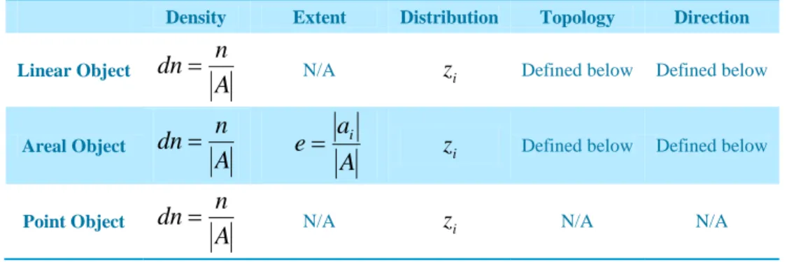
Due the wide differences in their construction, e.g. an areal object extends over a large area, whereas a point object is simply a single point within the polygon, not all the different as-pects mentioned above are applicable to every type of spatial object. Table 1 lists the different types of characteristics applicable to the different types of spatial objects.

In Table 1, n is the number of times the spatial object occurs within the polygon, A is the total area of the polygon, a_i is the total extent of the areal object

i

within the polygon, and

i

z is the test statistic obtained from the Mean Nearest Neighbor test for complete spatial random-ness (CSR) ( Donnelly 1978), and N/A stands for not applicable. Next, we define the functions that are used to find the distance between two polygons on the basis of the above mentioned properties of the spatial objects present within the polygons.

(37)

Table 1:Different characteristics of spatial object attributes

Density Extent Distribution Topology Direction Linear Object

A

n

dn



N/A z_i Defined below Defined below

Areal Object

A

n

dn



A a

e i z_i Defined below Defined below

Point Object

A

n

dn



N/A z_i N/A N/A

Density and Extent. Density is the number of times an object occurs within a polygon divided by the area of the polygon. Extent is the total area covered by the object within the poly-gon. We measure the distance between two polygons on the basis of the density of the objects using Equation 7, and on the basis of extent using Equation 8.

) , max( i j j i density dn dn dn dn d   (7)

where dn_i is the density of point object m in polygon

P

_i, dn_jis the density of point

ob-ject m in polygon P_j. ) , max( _i _j j i extent e e e e d   (8)

where e_iis the total extent of an areal object within polygon

P

_i, e_jis the total extent of the areal object within polygon P_j.

Distribution. The spatial distribution of an object is measured using the Mean Nearest Neighbor test for complete spatial randomness (CSR) (Donnelly 1978 ). The statistic produced as the output of this test is a fair indicator of the presence of aggregation, regularity or randomness

of events located within a polygon. This information about the polygons helps us in identifying the polygons that have a similar underlying structu