The Need for Speed: Minimum Quote Life Rules and Algorithmic
Trading
Alain Chaboud Erik Hjalmarsson Clara Vega
[PRELIMINARY AND INCOMPLETE. PLEASE DO NOT CITE.] May 4, 2015
Abstract
We study the impact that a minimum-quote-life (MQL) rule of 250 milliseconds in the euro-dollar currency pair had on trading volume, bid-ask spreads, market depth, and adverse selection costs for “slow”traders. We …nd that the MQL rule causes trading volume to decline in the EBS trading platform, suggesting that some market participants may have moved to other trading venues without MQL rules. In addition, we …nd that the MQL rule did not have an impact on average bid-ask spreads, which suggests that the counterbalancing e¤ects of lower adverse selection costs and higher market-making costs for HFTs play a role in a way that they cancel each other out. However, the MQL might have increased bid-ask spreads in volatile times. The impact on depth is inconclusive. We also …nd some (weak) evidence that HFTs are less willing to provide liquidity during volatile times after the MQL rule was implemented. Finally, consistent with the recent theoretical literature on HFT, we …nd that “slow”traders pay a premium (adverse selection cost) when they transact with better informed high-frequency traders, and that these costs declined after the MQL rule was implemented.
JEL Classi…cation: F3, G12, G14, G15. Keywords: Algorithmic trading; Price discovery. Chaboud and Vega are with the Division of International Finance, Federal Reserve Board, Mail Stop 43, Washington, DC 20551, USA; Hjalmarsson is with University of Gothenburg, Department of Economics and Centre for Finance, Vasagatan 1, SE 405 30 Gothenburg, Sweden, and Queen Mary University of London, School of Economics and Finance, Mile End Road, London E1 4NS, UK. Please address comments to the authors via e-mail at [email protected], [email protected], and [email protected]. We are grateful to EBS/ICAP for providing the data. We have bene…ted from the comments of Ola Bengtsson, Johannes Brecken‡eder, Jungsuk Han, Chester Spatt, Per Strömberg, and of participants in the Lund University Finance Seminar, and the Swedish House of Finance Seminar. The views in this paper are solely the responsibility of the authors and should not be interpreted as re‡ecting the views of the Board of Governors of the Federal Reserve System or of any other person associated with the Federal Reserve System.
1
Introduction
Recent theoretical papers suggest that “fast”or high-frequency traders (HFTs) may have a negative
impact on market quality. Speci…cally, Foucault, Hombert and Ro¸su (2013), Budish, Cramton and
Shim (2013), and Biais, Foucault, and Moinas (2013), among others, argue that the participation of HFTs may reduce market liquidity due to increased adverse selection costs. Consistent with this negative view, …nancial market regulators and trading platforms have recently implemented policies with the intention of “slowing down”HFTs. In this paper, we analyze the impact of one of these policies, the implementation of a minimum-quote-life (MQL) rule of 250 milliseconds for the euro-dollar currency pair, on June 15, 2009, by the Electronic Broking Services (EBS) FX trading platform.
We rely on a novel data set consisting of several years (Jan 2008 to December 2010) of high-frequency transaction and quote data from EBS. The data represent a large share of spot interdealer transactions across the globe in the euro-dollar currency pair, with EBS widely considered to be the primary site of price discovery in this exchange rate during our sample period. A crucial feature of the data is that, on a second-by-second frequency, the volume and direction of transactions of manual (slow), Bank-AI (fast), and PTC-AI (fastest) traders are explicitly identi…ed, allowing us
to measure changes in their respective behavior due to the MQL rule.1
We …rst use our data to study the impact of MQL on trading volume. Theory predicts coun-terbalancing e¤ects. The posting of a limit order essentially provides a free option to the market to trade at the price posted. The value of an option is increasing in its time-to-maturity, and an MQL rule e¤ectively imposes a lower bound on this time-to-maturity. Thus, the MQL rule makes the option provided by the limit order more valuable, and market making thereby becomes more expensive (or risky). The MQL rule we study, a 250 milliseconds minimum resting time, only a¤ects
the ability of algorithmic and high-frequency traders to cancel their posted quotes.2 We thus expect
the MQL rule to have the biggest impact on the behavior of “fast” traders. Some “fast” traders,
1In the EBS trading platform, traders can enter trading instructions manually, using an EBS keyboard, or, upon approval, via a computer directly interfacing with the system, what EBS labels automated interface (AI) traders. EBS further breaks down AI traders into two groups, “Professional Trading Community”(PTC) traders and “Banks.”PTC traders are hedge funds and CTAs (commodity trading advisors). These traders, according to EBS, are traders with the lowest latency, or what the media refers to as high frequency traders. In our analysis we classify manual traders as slow, Bank-AI as fast, and PTC-AI as the fastest.
2
EBS indicated to us that there is no manual trader in the EBS trading platform who is able to post and cancel an order in less than 250 milliseconds. This makes sense as the blink of a human eye lasts approximately 400 milliseconds.
for example, may decide to go to other trading venues, where market making is less expensive from their point of view. As a result, some of the “slow” market participants may also leave because the “fast” market participants, who provided a market making service, left. Thus, the MQL rule may cause a decline in overall trading volume because of the departure of several types of market participants.
In contrast to the option theory, Foucault, Hombert and Ro¸su (2013), Budish, Cramton and
Shim (2013), and Biais, Foucault, and Moinas (2013) highlight that the speed advantage of HFTs— the ability to post and cancel quotes quickly— gives HFTs an informational advantage. The MQL rule takes away this informational advantage from HFTs, thereby lowering adverse selection costs for “slow” traders. The impact that lower adverse selection costs for “slow” traders has on trading volume is ambiguous. Trading volume may increase if the arrival of new “slow” traders due to lower adverse selection costs is bigger than the departure of HFTs because they do not have an informational advantage any more. To investigate the impact MQL had on trading volume, we use a di¤erence-in-di¤erences methodology using trading volume in the futures market as the comparison group. We …nd that trading volume in EBS declines relative to trading volume in the futures market. Interestingly, we …nd evidence of an increase in trading volume in the futures market, suggesting that some market participants may have moved to the futures market following the implementation of the MQL rule in the spot market.
We next study the impact of MQL on bid-ask spreads and market depth (i.e., the quantity available to trade at posted quotes). Similar to the predictions related to trading volume, theory predicts counterbalancing e¤ects. Option theory predicts that the MQL rule will cause market making to be more expensive or risky for HFTs, which in turn implies that the HFT market-makers, who decided to stay in the EBS market, may demand a higher compensation for their market-making services by posting wider bid-ask spreads and perhaps providing less depth at the top of the limit order book. Also, market-making competition may be lower after the implementation of the MQL rule, because some HFTs may leave the market as conjectured above, which in turn would increase bid-ask spreads (Li (2013)). However, the MQL rule might also lower competition amongst aggressive HFT liquidity demanders, as the MQL rule takes some of their informational advantage away from them, and lower competition amongst this type of HFTs would lower bid-ask spreads, as Breckenfelder (2013) shows. As explained above, this type of HFTs leaving the market would also
lower adverse selection costs. These latter two e¤ects would cause bid-ask spreads to decline and market depth to increase. Our di¤erence-in-di¤erence estimation shows that, on average, MQL had little, or no, impact on bid-ask spreads, suggesting that the counterbalancing e¤ects play a role in a
way that they exactly cancel each other out.3 The results for market depth are harder to interpret,
with a large increase in depth on the EBS market subsequent to the MQL implementation, but an even larger increase is seen in the Futures market, resulting in a negative di¤erence-in-di¤erence e¤ect. Taken at face value, the di¤erence-in-di¤erence would thus suggest that the MQL rule had a (large) negative impact on market depth. However, given that both the EBS and futures market in fact exhibited great increases in depth around the implementation of the MQL rule, it is di¢ cult to put much faith in the di¤erence-in-di¤erence result for depth.
Option theory predicts that the e¤ect of an MQL rule might be particularly noticeable during
volatile times. The value of an option increases with time to maturityand volatility. Thus, the value
(or cost) of the imposed minimum time-to-maturity will be largest in times of high volatility. Since volatile times might be associated with times of market stress, these are arguably the periods during which the access to liquidity is most important. An MQL rule, however, is likely to make liquidity provision in volatile times relatively scarcer. We …nd some weak evidence that high-frequency traders are less willing to provide liquidity during volatile times, but these results are only seen in the shortest time window immediately following the MQL implementation. Over longer windows, this results is no longer present. We do, however, …nd relatively strong and consistent evidence that bid-ask spreads are slightly higher during volatile times after the MQL rule is implemented in the system.
Finally, we investigate further the idea that “slow” traders pay a premium (adverse selection cost) when they transact with better informed high-frequency traders, as predicted by the theoretical
papers of Hombert and Ro¸su (2013), Budish, Cramton and Shim (2013), and Biais, Foucault,
and Moinas (2013). To expore this possibility we estimate the e¤ective spread (di¤erence between the transacted price and the mid-quote) paid by di¤erent types of traders, slow, fast and fastest, when they are trading with high-frequency or the “fastest” traders. We …nd that both the “slow”
3
Another possibility is that the 250 ms minimun-resting-time for orders is too short to have any impact on the market. We rule this possibility out by showing that MQL did have an impact on trading volume. We also show that the 250 ms MQL rule is binding, i.e., prior to the implementation of the rule there were several market participants who cancelled their quotes within 250 ms. Below, we also show that MQL did have an impact on adverse selection costs for “slow” traders.
traders and the “fast” traders pay an e¤ective spread that is approximately 0.2 pips higher than
the spread paid by the “fastest”traders (the average spread is of an order of 1 pip).4 One can view
these di¤erences in e¤ective spreads as compensation for HFT’s investment in technology, and a social planner may not …nd the same e¤ective spread across all trader categories to be optimal, as previous studies show that traders bene…t from the presence of algorithmic traders (e.g., Chaboud, Chiquoine, Hjalmarsson, and Vega (2014) …nd that algorithmic trading participation increases the informational e¢ ciency of prices and Hendershott, Jones, and Menkveld (2011) …nd that algorithmic traders improve market liquidity). Nevertheless, we test the hypothesis, suggested by the theoretical literature, that an MQL rule may lower adverse selection costs for “slow” market participants, and compare e¤ective spreads paid by di¤erent types of traders before and after the MQL rule. We …nd evidence that there is a small decline in e¤ective spreads paid by “slow”traders after the MQL rule implementation. In other words, the MQL rule might have accomplished what EBS intended to do, namely to lower adverse selection costs for “slow” traders.
The paper proceeds as follows. In Section 2, we brie‡y discuss the related empirical literature on the impact of policies aimed at slowing down high frequency traders. Section 3 introduces the high-frequency data used in this study, and o¤ers a short description of the structure of the market. Section 4 shows that the 250 millisecond rule was indeed binding for some market participants and in Section 5, we test whether there is evidence that the MQL rule had a causal impact on trading volume, bid-ask spreads, and depth. Section 6 discusses whether trading volume by computers were di¤erently a¤ected by the MQL rule than human trading volume. Section 7 investigates conditional volatility e¤ects of the MQL rule and, Section 8 consider the possibility that “slow” traders pay an adverse selection cost premium when transacting with high-frequency traders, and whether this adverse selection cost goes down after the MQL rule was implemented. Finally, Section 9 concludes.
2
Related literature
The posting of a limit order essentially provides a free option to the market to trade at the price posted. Classical option theory therefore provides some basic ideas of the e¤ects of an MQL rule.
4An alternative explanation is that high-frequency traders provide liquidity to other market participants when liquidity is expensive. We rule out this explanation because we compare e¤ective spreads paid by di¤erent types of traders after controlling for the inside quoted spread.
The value of an option is increasing in its time-to-maturity, and an MQL rule e¤ectively imposes a lower bound on this time-to-maturity. Thus, the MQL rule makes the option provided by the limit order more valuable, and market making thereby becomes more expensive (or risky). Since the primary compensation for market making activities is collected through the bid-ask spread, all else equal, one would expect the bid-ask spread to increase after the imposition of an MQL rule. Somewhat more speculatively, one might also expect that depth decreases, as a result of a decreased willingness to post quotes. To the extent that alternative trading venues exist, one might also posit a decrease in overall transacted volume, as market participants move to “cheaper” platforms. The implications from classical theory are thus quite negative, and this view is re‡ected in normative
statements by many leading academics.5
Another immediate implication of classical option theory is that the e¤ect of an MQL rule might be particularly noticeable during volatile times. The value of an option increases with time
to maturityand volatility. Thus, the value (or cost) of the imposed minimum time-to-maturity will
be largest in times of high volatility. Since volatile times might be associated with times of market stress, these are arguably the periods during which the access to liquidity is most important. An MQL rule, however, is likely to make liquidity provision in volatile times relatively scarcer.
The above insights would appear quite general, in the sense that they derive from essentially model-free results in option theory. However, these implications are likely best seen as the outcome of a comparative static analysis, where the liquidity conditions in a market with pre-dominantly high-frequency market makers is compared before and after an MQL rule is imposed. In a recent theory paper, Han, Khapko, and Kyle (2014) analyze the equilibrium bid-ask spread in a simple model where there may or may not be high-frequency market makers present in the market. If the probability of high-frequency order posting is equal to one, this results in bid-ask spreads that are always smaller or equal to those observed in the case without high-frequency market makers
(i.e., probability of high-frequency order posting equal to zero).6 In a situation where high-frequency
5
The following quotes sum up well the scepticism of MQL rules among many academics. “The independent academic authors who have submitted studies are unanimously doubtful that minimum resting times would be a step in the right direction. . . ” (Linton, O’Hara, and Zigrand in Foresight); “This will result in a dry up of liquidity in the book and might even cause an increase in volatility. To be honest, we think this proposal is a terrible idea. . . ” (Farmer and Skouras, in Foresight); “However, the minimum time-in-force appears to be a particularly blunt, poorly considered tool.” (Jones, 2013).
6
This essentially con…rms the discussion above, since the known absence or presence of high-frequency market makers can be viewed as analogous to a real-world situation with or without an MQL rule in place. In practice, the exact time-constraints imposed on order withdrawals by the MQL rule will, of course, have di¤ering implications.
participation is possible but not certain, these unambiguous implications no longer hold, and bid-ask spreads might at times, and on average, end up higher than in the case where there is no high-frequency participation for certain. This re‡ects the additional adverse selection risk faced by the low-frequency makers, since they are not able to update their quotes in the case of new information arrivals, unlike the high-frequency makers. In this case, the imposition of an appropriate MQL
rule couldlower average bid-ask spreads by essentially bringing the market (closer) to the situation
where there is no high-frequency participation.
Another intuitive implication of an MQL rule is that prices might become less informationally e¢ cient, as market makers are restricted in updating their quotes given new available information. Given the very short time-horizons that might be a¤ected by any MQL rule in modern markets (e.g., 250 milliseconds in the EBS case), this potential ine¢ ciency is perhaps not of great importance, but highlights once again the trade-o¤ between e¢ ciency and adverse selection that has been a common theme throughout much of the theoretical literature on high-frequency trading.
3
Market structure and data description
3.1 The EBS interdealer market
Global interdealer spot trading in major currency pairs (exchange rates) is dominated by two dif-ferent trading platforms: Electronic Broking Services (EBS) and Reuters. The euro-dollar trade primarily on EBS, and the price-discovery process for this currency pair is therefore concentrated to the EBS trading platform. Prices on EBS constitute the reference for derivative pricing and dealer quotes in these currencies. The EBS system is an interdealer system accessible to foreign exchange dealing banks and, under the auspices of dealing banks (via prime brokerage arrangements), to hedge funds and commodity trading advisors (CTAs). EBS controls the network and each of the terminals on which the trading is conducted. The minimum trade size over our sample period is 1 million of the “base” currency (i.e., the euro in our case), and trade sizes are only allowed in multiple of millions of the base currency.
On June 15, 2009, EBS imposed a so-called minimum-resting-time, or minimum-quote-life
However, in a highly stylized model such as the one studied by the Han, Khapko, and Kyle (2014), the analogy seems valid, and the authors themselves partly intepret their results in light of minimum quote life rules.
(MQL) rule, of 250 milliseconds for the euro-dollar currency pair. Speci…cally, this new rule speci-…ed that any limit order posted on the euro-dollar market could not be withdrawn within the …rst 250 milliseconds of its posting. The MQL rule was implemented on a Monday (June 15, 2009), and took full e¤ect immediately; i.e., there was no transition period of any sort. The MQL rule and its implementation date was, as far as we are aware, known in advance to market participants. However, as described below, there is no empirical evidence that market participants changed their
behavior prior to the actual implementation of the MQL rule on June 15, 2009. It should also be
pointed out that no other changes to the EBS market structure was implemented at, or around, the date of the MQL implementation.
Concurrent media reports suggested that EBS implemented a minimum quote life in order to (i) avoid, or at least limit, “‡ickering quotes”, (ii) promote genuine “intent-to-trade”, (iii) improve the “…ll-ratio”(i.e., the ratio of executed quotes to submitted quotes), and (iv) “level the playing …eld” between human and computer traders. All of these arguments can be viewed as “soft”considerations that were likely motivated by a desire to appease human traders on the EBS trading platform.
3.2 Data description
Our primary data are obtained from the EBS trading platform, but in order to conduct a com-parative di¤erence-in-di¤erence analysis, we also use data from the Chicago Mercantile Exchange (CME) futures market. These data sets are described in detail below.
3.2.1 High-frequency EBS quote and volume data
From Jan 2008 until June 2010, we have detailed intra-daily data on quotes and transacted amounts
(i.e., the volume of trade measured in the base currency).7 The quote data provide the highest
bid quote and the lowest ask quote on the EBS system in a given currency pair. All quotes are executable, and therefore represents the market price at that instant. In addition, the amount available for trade at both the highest bid and the lowest ask price are recorded (i.e., the depth at the inside quotes), as well as the amounts available, on the bid and ask side separately, for quotes at 2, 3, and 5 basis points away from the inside bid and ask quotes. The total depth (sum of the depths at the bid and the ask quotes) at the inside quotes will be referred to as depth0, and the
7
depths 2, 3, and 5 basis points away are labeled depth2, depth3, and depth5, respectively.
The transactions data provide detailed information on the volume and direction of trade. In particular, for each time-interval, we observe both the total volume of trade, as well as the buy and sell amounts from the perspective of the taker. That is, the direction of trade is based on actual
trading records: A trade is recorded as, for instance, buyer-initiated, if it is the result of a ‘hit’on
a posted ask quote.
On the EBS trading platform, traders can enter trading instructions manually, using an EBS keyboard, or, upon approval, via a computer directly interfacing with the system. EBS, in turn, records whether a trade was placed by an ordinary keyboard interface, or by a direct computer in-terface, allowing for a classi…cation of trades into “human”or “computer”trades. This classi…cation into human and algorithmic (computer) trading formed the basis for the recent study by Chaboud, Chiquoine, Hjalmarsson, and Vega (2014). While we are also able to classify trades as human or computer trades, our data actually allows for an even …ner classi…cation of trades. In particular, in this more recent data (starting in 2008), EBS decomposes the computer (algorithmic) volume into two di¤erent categories, referred to as Bank-AI and PTC-AI, where PTC stands for Profes-sional Trading Community and AI for Automated Interface, which is how EBS labels the direct computer interfaces. The “Professional Trading Community” essentially refers to hedge funds and CTAs (commodity trading advisors), which can trade directly on EBS under the auspices of dealing banks via prime brokerage arrangements. That is, in our data we are not only able to distinguish whether trading was conducted by a human or a computer, but also, in case of a computer, whether that computer was in the employ of a bank or the professional trading community. Speci…cally, for each observed time-interval we observe the volume attributable to all nine possible combinations of human, Bank-AI, or PTC-AI maker or taker, with the direction of trade from the perspective of the taker explicitly identi…ed.
The transactions data and depth data described above are aggregated by EBS and are available at a one-second frequency throughout our sample period. The actual quote data are also available at the second-by-second frequency throughout the sample period, although we also have access to quote data that are sampled every 100ms during the year 2009. These latter 100ms data are used in analyzing transaction level data, as described in the following subsection.
3.2.2 Millisecond time-stamped EBS transaction records
In addition to the longer sample of one-second data on quotes and transacted volumes, we also have access to a somewhat shorter sample of individual time-stamped trades, spanning all of 2009. These data record the time-stamp, with millisecond precision, of each trade that occurred, along with the actual transaction price. The amount transacted, and the direction of the trade from the taker perspective, is also recorded. Importantly, the nature of the maker and taker of the trade is explicitly identi…ed, using the three di¤erent categories described above (Human, Bank-AI, and PTC-AI). Thus, each trade is classi…ed according to nine di¤erent possible combinations of maker and taker, as well as with an indicator of whether the taker was the buyer or the seller.
These millisecond time-stamped transactions data are lined up with the 100ms quote data, such that for a given transaction, the best bid and ask prices prevailing at the nearest previous whole 100ms interval are also available. That is, the quote data are “lagged” up to 99ms for a given
recorded transaction.8 In additions, the depth available at the nearest previous whole second is also
lined up with the transaction level data, in order to provide as complete and timely a picture as possible of prevailing market conditions at the time of a given transaction.
3.2.3 Daily CME futures data
Further, we also use data from the CME futures exchange, where futures contracts on the euro-dollar currency are traded. In particular, we have data on daily trading volume (in the base currency), the daily average bid-ask spread at the best bid and ask quotes, and the daily average of the depth available at these quotes (i.e., the sum of the depths at the bid and ask quotes, corresponding to depth0 in the above EBS data). These data are also available from Jan 2008 through June 2010.
The trading activity on the futures market is a¤ected by the “roll-cycle”of the futures contracts, which leads to a very clear “intra-cycle” seasonality in futures trading volume. Since changes in trading volume due to this roll-cycle is not of explicit interest, we also construct roll-adjusted futures volume series. In particular, as speci…ed above, at a given point in time, we use trade data for a speci…c futures contract with a speci…c expiry date. We can therefore create a series of dummy variables that indicate the number of weeks to expiry at a given observation date. In particular,
8
Given inherent latencies in the system, the 100ms-frequency quote data lined up with a given transaction is likely as representative a bid and ask price that one can feasibly achieve.
for any observation, there is between 1 and 13 weeks to expiry for the contract currently used to construct our data. Our series of futures volume is regressed on these 13 dummy variables, and the residuals are computed. The roll-adjusted volume series is de…ned as these residuals plus the average non-adjusted volume; the adjusted and non-adjusted series thus have identical means.
The daily futures data is merged with aggregated daily EBS data. In particular, the one-second EBS quote and volume data are aggregated into a daily data set, where the bid-ask spread and depth variables are averaged across all observations within the day. The traded volume is summed up over the day, to correspond with the daily futures volume. This merged data set spans from Jan
3, 2008 to June 30, 2010, for a total of 618 daily observations.9
4
Was the MQL rule binding?
Before conducting any further analysis, the most fundamental question that needs answering is whether the MQL rule was actually binding. That is, prior to the implementation of the MQL rule, did market makers on EBS to any relevant degree cancel quotes within 250 milliseconds of their posting? In order to address this question, we use a separate data set on quote submissions and quote interruptions on the EBS platform. In particular, we have access to daily data, from January 5, 2009 to December 30, 2009, on the total number of submitted and cancelled quotes in the euro-dollar market on the EBS system. Crucially, in terms of evaluating whether the MQL rule
was truly binding, we also have daily data for the number of quotes cancelled within 250ms of their
posting.
As seen from Figure 1, it is very clear that the MQL rule was indeed binding. Figure 1 show time-series plots of the daily fraction of all submitted quotes on EBS that were cancelled prior to 250 milliseconds, before and after the implementation of the MQL rule. In particular, daily data from January to December 2009 are shown, with the MQL implementation occurring in the middle of the sample, on June 15, 2009. Due to the highly proprietary nature of these data, the actual
9
We exclude data collected from Friday 17:00 through Sunday 17:00 New York time from our sample, as activity on the system during these “non-standard” hours is minimal and not encouraged by the foreign exchange community. Trading is continuous outside of the weekend, but the value date for trades, by convention, changes at 17:00 New York time, which therefore marks the end of each trading day. We also drop certain holidays and days of unusually light volume: December 24-December 26, December 31-January 2, Good Friday, Easter Monday, Memorial Day, Labor Day, Thanksgiving and the following day, and July 4 (or, if this is on a weekend, the day on which the U.S. Independence Day holiday is observed).
scale cannot be shown in the …gure, but rather the data are indexed such that the euro-dollar series starts at an index value of 100 on the …rst day of the sample. However, to give an approximate idea of the scale in the graph, the fraction of all submitted quotes that were cancelled within 250 milliseconds of their posting was typically between 10 and 15 percent, prior to the implementation of the MQL rule. After the implementation of the MQL rule, this cancellation rate naturally drops to (almost) zero. After the MQL rule was put in place, there is still a tiny fraction of quotes that are recorded as cancelled before the 250 milliseconds mark. According to EBS, this is essentially a recording error that can sometime occur when quotes are cancelled as close to the 250 milliseconds mark as possible.
Thus, prior to the implementation of the MQL rule, a sizeable fraction of all quotes (of the order of 10 percent) were cancelled within 250 milliseconds of their posting. The MQL rule was, in this sense, clearly binding to many market participants. Figure 1 also shows that there is no evidence that market makers altered their behavior prior to the actual enforcement of the MQL rule. That is, there is no gradual drop in cancellation rates in the period leading up to the MQL implementation date, but rather a very steep fall from the day prior to the day of the enactment of the rule. Taken together, these …ndings motivate a further analysis of the impact of the MQL rule, on market characteristics beyond the mere cancellation rates documented here. The sharp drop, and lack of gradual adjustment, in quote cancellations, also motivate a “before-after” analysis, where market conditions right before the implementation of the MQL rule is compared to conditions immediately afterwards.
Figure 2 provides some further evidence on the quoting and trading behavior on EBS, in the period around the implementation of the MQL rule. In particular, the graphs in Figure 2 show daily aggregates of (i) the number of submitted quotes and the (ii) the number of interrupted quotes (i.e., quotes that do not result in a trade). Similar to Figure 1, in each panel the series are
indexed such that they begin at 100.10 Given the evidence in Figure 1, the most striking feature
of the graphs in Figure 2 is the lack of any clear e¤ect at the time of the MQL implementation. Indeed, neither of the two variables plotted in Figure 2 show any clear and consistent reaction to the MQL implementation. There is perhaps some suggestive evidence of a break around the MQL
1 0
The series in the two panels in Figure 2 look virtually identical. This is due to the fact of the high order cancellation rates in electronic limit order markets, where the vast majority of orders are cancelled before leading to a trade.
implementation, although this is di¢ cult to establish given the high day-to-day variance in the data. In any case, any such potential e¤ect appears to have been short-lived.
Table 1 explores this notion further. The table shows the change in averages of the
log-transformed variables from 10, 30, or 60 days prior to the implementation of the MQL rule to 10, 30, or 60 days after the implementation. That is, the table shows the average log-values in the 10 (30, 60) days immediately following the MQL implementation, minus the average log-values in the 10 (30, 60) days immediately prior to the MQL implementation. This after-minus-before value thus provide an estimate of the change from before to after the MQL implementation. Although some of the estimated changes are statistically signi…cant, there is little consistency across time horizons (10, 30, or 60 days before and after). In particular, both the number of submitted and interrupted quotes seem to have dropped by about 15 percent in the period immediately following the implementation of the MQL rule, consistent with the idea that the orders that were previously posted and cancelled in less than 250 milliseconds did not get posted at all after the implementation of the MQL rule. However, if such an e¤ect did occur, it appears to have been very short-lived, as the same pattern cannot be seen at the 30- and 60-day horizons. Thus, apart from some evidence of a short-run e¤ect, the results in Table 1 mostly con…rm the visual evidence in Figure 2, namely that the MQL rule did not have any clear and obvious impact on the quoting behavior on EBS.
5
Daily before-after analysis
In the …rst part of the empirical analysis, we compare the daily average bid-ask spread, daily depth, and total daily volume before and after the implementation of the MQL rule. This is done both in a simple after manner, as well as in a “di¤erence-in-di¤erence” manner, where the before-after outcome on the EBS trading platform is compared to the before-before-after outcome on the CME Futures market (which was not subject to an MQL rule). By di¤erencing out any common e¤ects in these two markets, a clearer estimate of the impact of the MQL rule is obtained. After a graphical presentation of the data, we present comparisons of unconditional averages in a simple di¤erence-in-di¤erence analysis, and then further verify those …ndings in a regression-based formulation of the di¤erence-in-di¤erence model, where secular trends and observable factors are controlled for.
5.1 Graphical evidence
The top panel in Figure 3 plots the average daily (inside) bid-ask spreads on EBS from Jan 2008 to June 2010. The series are logged and standardized to each start at a value of 100, such that a comparison of relative changes over time can easily be done. The EBS spread is on a downward
trend at the time of the MQL implementation. There is no strong indication that this trend
is altered around the MQL implementation, although there is perhaps some suggestion that the decrease in spreads become more prominent after the implementation of the MQL rule. As a point of comparison, the spreads in the Futures market are also shown in Figure 3. The observed patterns in the futures market are qualitatively similar to those on EBS, with a downward trend around the MQL implementation. There is again no clear sign of any break around the MQL implementation, which might be expected since the futures market was not directly a¤ected by the MQL rule.
Although an impact on the bid-ask spread is probably the clearest prediction coming out of the classical option theory, one might also conjecture that the posted depth in the market is a¤ected by an MQL rule. That is, the increased cost of posting quotes might lead to a smaller depth. The bottom panel of Figure 3 show graphs of the standardized average daily depth available at the inside spread (i.e., depth0 in the above notation). Again, there is no obvious impact around the MQL implementation, although there might be some indication that depth is rising a bit more sharply after the MQL implementation. As is seen, depth is also trending strongly upwards on the futures market around the time of the MQL implementation.
Overall, there is thus no completely clear graphical evidence that the MQL rule a¤ected average bid-ask spreads or depths. However, the graphs presented in Figure 3 still leaves open the possibility that the MQL rule did have some impact on spreads and depths, an we present more formal results in the di¤erence-in-di¤erence analyses below.
The top panel of Figure 4 show time-series plots of the daily total volumes on EBS and the Futures market, from Jan 2008 to June 2010. The series are logged and standardized to each start at a value of 100. The bottom panel of Figure 4 show the same plots, but using the roll-adjusted Futures volume, described in the data section above. As is evident from both …gures, the EBS and the Futures volumes exhibit very similar patterns over time, and co-vary strongly with each other. However, after the implementation of the MQL rule on EBS, there appears to have
been a noticeable shift in these patterns, with an increase in Futures volume that is not matched by a similar increase in EBS volume. The graphs in the top panel of Figure 4, which show the unadjusted futures volume, suggest that this shift started before the implementation of the MQL rule, but the roll-adjusted volumes in the bottom panel indicate that the shift appears to actually
have happened right around the implementation of the MQL rule.11;12 These graphical evidence are
certainly suggestive of an impact of the MQL rule on overall market activity. In particular, they suggest that, at least in relative terms, the trading volume on EBS might have decreased as a result of the MQL implementation.
5.2 Di¤erence-in-di¤erence mean analysis
Let yEBS;t represent either the average bid-ask spread, depth, or the total trading volume in the
EBS market at time t = 1; :::; T, and let yF ut;t be the corresponding daily measure in the CME
Futures market. In order to gauge the impact of the MQL rule, a di¤erence-in-di¤erence analysis is used,
dd= (yEBS;af ter yEBS;bef ore) (yF ut;af ter yF ut;bef ore): (1)
Here, yi;af ter, i2 fEBS; F utg, is the mean of yi;t over the period after the MQL implementation,
and yi;bef oreis the mean ofyi;t over the periodbefore the MQL implementation. In order to isolate
the e¤ect of the MQL rule, only data relatively close to the event date are used to calculateyi;af ter
yi;bef ore. In particular, windows spanning from 10, 30, or 60 days before the MQL implementation
to 10, 30, or 60 days after, respectively, are considered.
Table 2 provides results on the log-changes in the data around the implementation of the MQL rule. In particular, the table shows the change in average log-spread (log-depth, log-volume) from 10, 30, or 60 days prior to the implementation of the MQL rule to 10, 30, or 60 days after the implementation. That is, the table shows the average log-spread (log-depth, log-volume) in the 10 (30, 60) days immediately following the MQL implementation, minus the average log-spread (log-depth, log-volume) in the 10 (30, 60) days immediately prior to the MQL implementation. Changes
1 1The implementation of the MQL rule on EBS coincided with an expiry date in the futures market. The di¤erence between the un-adjusted and roll-adjusted futures volume is therefore quite noticeable on the date of the MQL implementation. As discussed in the data section, the change over time in the roll-adjusted volumes should provide a better measure of changes in trading activity in the futures market that is not explicitly linked to the roll-cycle.
1 2
The e¤ect of the roll-cycle on the bid-ask spread and the depth is much more limited, and the graphs for the bid-ask spread and depth therefore only show the unadjusted futures data.
are shown both for EBS and Futures data. In the results for trading volume, the Futures results are either based on unadjusted (left-hand-side column) or roll-adjusted (the right-hand-side column) volumes. In addition, the di¤erence between the log-change in the EBS data and the Futures data are shown in the bottom rows of each panel in the table. These “di¤erence-in-di¤erence” results thus correspond to estimates of equation (1). Standard errors are shown in parentheses below each estimate; the rows labeled Historical 90% conf. int. are described in Section 5.2.3 below.
5.2.1 Bid-ask spreads and depth
The results for the bid-ask spread and depth0 are shown in the …rst two columns of Table 2, and mostly re‡ect the graphical evidence presented in Figure 3. Over the short 10-day before to 10-after period around the MQL implementation, there is no statistically signi…cant change in either of these variables, but over the longer 30- and 60-day before-after windows, there is a clear decrease in the EBS spreads and increase in the EBS depths. The same pattern holds for the futures data, however, where the log-changes in spreads and depths are greater in absolute magnitude than on EBS. The di¤erence-in-di¤erence estimates are therefore positive for spreads and negative for depth, suggesting that when viewed relative to the futures market, there might have been an increase in spreads and a decrease in depth on EBS in the 30- and 60-day windows following the MQL implementation.
Since all estimates represent log-changes, they can be interpreted as approximate percentage changes. In the 30- and 60-day windows following the MQL implementation, the bid-ask spread decreased by approximately 4 and 8 percent, respectively, compared to the 30- and 60-day windows prior to the MQL implementation. During the same periods, the corresponding decrease in the Futures spread was around 9 and 12 percent, such that the futures market spread decreased by approximately 4 percentage points more than the EBS spread. The changes in depth on the EBS market were around 4 and 12 percent in the 30- and 60-day before-after windows. The futures market, on the other hand, exhibited 24 and 47 percent increases in depth over the same periods. Depth on EBS, relative to the futures market, therefore decreased by 20 and 35 percent in the 30 and 60 before-after window. These massive increases in depth in the futures market over the event period makes it rather di¢ cult to interpret the di¤erence-in-di¤erence estimates.
Moreover, in absolute terms, the EBS spread decreased and the depth increased following the MQL implementation. The purpose, of course, of a di¤erence-in-di¤erence analysis is to eliminate
any common factors that might be present, and thus isolate the actual “treatment”e¤ect. Still, the interpretation becomes a bit more di¢ cult when the absolute change on the treated market goes in the opposite direction of the di¤erence-in-di¤erence estimate.
5.2.2 Total volume
The estimates of the change in average volume on the EBS platform around the MQL implementa-tion, shown in the top rows in each panel in Table 2, tell a fairly clear story. The implementation of the MQL rule appears to have been associated with a fairly large drop in overall volume on EBS.
Average euro-dollar volumes appears to have dropped around16to18percent in the period around
the MQL implementation. The unadjusted volumes in the futures market also drop substantially in the 10 days following the MQL implementation, compared to the 10 days before. However, if one considers the 60-day before to 60-day after period, there is instead a substantial and statistically signi…cant increase in the futures volume after the implementation of MQL. These con‡icting results for the futures market are reconciled if one instead considers changes in the roll-adjusted futures volume. As seen in the right-most column of Table 2, there is now strong evidence of a substantial increase in futures volume at all horizons. The unadjusted and roll-adjusted results are, in fact, very similar for the 60-day before-after window. This is to be expected since the roll-cycle of futures contracts lasts for three months, or approximately 60 trading days. When considering averages over 60-day horizons, there is therefore hardly any impact of the roll-cycle, since it gets averaged out across the observations.
The …nal rows in each panel in Table 2 show the di¤erence-in-di¤erence estimates. That is, these are the di¤erences between the volume change on EBS and the volume change in the futures market. Using the roll-adjusted volume (shown in the right-most column), this di¤erence-in-di¤erence is large and statistically signi…cant. This, of course, follows from the decrease in EBS volume and increase in futures volume over the same period. With the unadjusted futures volume, the di¤erence-in-di¤erence is only clearly statistically signi…cant for the 60-day before-after window, which again is no surprise given the above discussion.
5.2.3 Statistical signi…cance
The results in Table 2, as well as the graphical evidence in Figure 4, suggest that the MQL rule had a negative impact on the trading volume on EBS. Perhaps a bit less convincingly, the evidence in Table 2 also suggest that relative to the futures market, the bid-ask spread on EBS increased and the depth decreased following the MQL implementation. Overall, the estimates of the mean changes shown in Table 2 tell a fairly clear story, but it is of course di¢ cult to properly ascertain their statistical signi…cance. The standard errors shown in ordinary parentheses below the point estimates in Table 2 are based on data for the 10- (30-, 60-) before-after period, and concerns about changes in the variance of the data over time might raise doubts about the validity of the standard errors.
In order to provide more robust evidence of signi…cant changes in the EBS market in association with the MQL rule, we construct the empirical distribution of the change in the EBS variables and the futures variables, using data only prior to the implementation of the MQL rule. In particular, starting at the beginning of the sample in Jan 2008, we calculate the change in average log-volume (log-spread, log-depth) from the …rst 10 days of the sample to the following 10 days; i.e., the change between days 1 through 10 and days 11 through 20. This is then repeated for every set of “10 plus 10” days in the sample, prior to the implementation of the MQL rule; i.e., for days 2-11 and days 12-21, days 3-12 and days 13-22, and so forth. The resulting collection of estimates provides an empirical distribution of the 10-day mean log-changes in trading volume at EBS. The last sub-sample end 10 days prior to the MQL event, such that there is no overlap with the data used to estimate the 10-day before-after results in Table 2. The same procedure is repeated for the futures volume, and for the 30-day and 60-day before-after windows, with the sampling ending 30 and 60 days prior to implementation of the MQL rule, respectively. Finally, the empirical distribution of the “di¤erence-in-di¤erence” estimates is also constructed analogously. That is, in this case, the di¤erence between the volume change on EBS and the volume change in the futures market is calculated for all 10- (30-, 60-) plus 10- (30-, 60-) day samples prior to the MQL rule, and the empirical distribution of these di¤erence-in-di¤erence estimates is obtained. The same procedure is applied to the bid-ask spread and the depth.
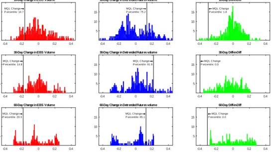
can then be used to evaluate how “abnormal” the change in volume (spread, depths) was around the MQL implementation. In Table 2, 90% con…dence intervals based on this historical empirical distribution are reported in square brackets. When viewed against the usual standard errors, shown in ordinary parentheses below the estimates in Table 2, the di¤-in-di¤ estimates for the 30- and 60-day before-after windows are signi…cant at the 5 or 1 percent level for both the spreads and the depths. If one instead compares the di¤-in-di¤ outcome to the arguably more robust con…dence intervals based on the historical empirical distribution, the spread results are no longer signi…cant whereas the depth results remain statistically signi…cant also under this more stringent evaluation. As seen in the …nal column of Table 2, the di¤-in-di¤ estimates for volume, using the detrended futures volume as control, are all statistically signi…cant according to the historical distribution. Figure 5 provides further evidence along these lines. In particular, Figure 5 shows plots of the empirical densities for the changes in euro-dollar EBS and roll-adjusted futures volumes, as well as the empirical densities of the di¤erence-in-di¤erence estimates. These plots also indicate the actual change around the MQL implementation, along with the percentile of the empirical distribution into which this change falls. It is evident that the drop in EBS volume around the MQL implemen-tation was unusual but not extreme. The change in volume around the MQL implemenimplemen-tation is roughly at the 15th percentile of the empirical distribution. However, this drop in EBS volume was associated with a large increase in futures volume, and the resulting di¤erence-in-di¤erence estimate falls in the extreme left tail of the di¤erence-in-di¤erence distribution. The results in Figure 5 thus suggest that the implementation of the MQL rule on EBS was associated with a moderate to large
decrease in EBS volume and a moderate to large increase in Futures volume. Looked at separately,
the changes in volumes on neither EBS nor the futures market appears extreme compared to the observed historical variation. However, when taken together, the simultaneous volume drop on EBS and volume increase in the futures market, does appear very extreme and highly statistically signif-icant. That is, when comparing the di¤erence-in-di¤erence estimates with the historical empirical distributions, they are all in the extreme left tail.
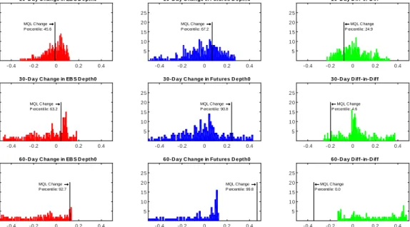
Figures 6 and 7 show the corresponding density plots for the historical changes in the log-spread and the log-depth, respectively. As seen in both of these …gures, and re‡ecting the results in Table 2, there is seemingly no impact of the MQL implementation of the 10-day before-after window. For the spread, this is true also for the 30-day before-after window, when judged against the historical
distribution. In the 60-day before-after window, however, both the EBS spread and depth exhibit large to extreme changes, but so do the corresponding Futures variables. In the spread case, this results in a di¤erence-in-di¤erence estimate that is in the middle of the historical distribution. In the depth case, the di¤erence-in-di¤erence estimate ends up in the extreme left tail. Based on the historical distribution, there is thus no statistically signi…cant evidence to suggest that the spread changed as a result of the MQL implementation.
Although the e¤ect on depth appears statistically signi…cant, the results presented in Figure 7 provide a much less convincing case of an actual MQL impact than does the results for volume presented in Figure 5. In the volume case, the absolute change on EBS is in the same direction as the di¤-in-di¤ estimate, and signi…cance of the di¤-in-di¤ estimate comes about through an unusual combination of a fairly large drop in EBS volume and a fairly large increase in Futures volume. In the depth case, both EBS and futures depth exhibit large to extreme positive changes, but the futures change is the most extreme, resulting in a negative and statistically signi…cant di¤erence-in-di¤erence estimate for depth.
5.3 The di¤erence-in-di¤erence analysis in regression format
The above di¤erence-in-di¤erence analysis strongly suggests that the implementation of the MQL rule was associated with a signi…cant simultaneous drop in EBS volume and increase in futures volume. There is little evidence to suggest a signi…cant and substantial impact on the average bid-ask spread, whereas the impact on depth is formally statistically signi…cant but open to interpretation. To provide further evidence along these lines, we re-write the di¤erence-in-di¤erence analysis in a regression format, which allows for the control of other possible factors that may have a¤ected trading volume around the date of the MQL implementation.
Using the same notation as previously, yi;t, i 2 fEBS; F utg, represents the log-volume
(log-spread, log-depth) in the EBS and futures market. The basic di¤erence-in-di¤erence analysis can be equivalently formulated in a regression format as follows,
yi;t = + M QLM QLi+ Af terAf teri;t+ DD(M QLi Af teri;t) + Xi;t+ i;t: (2)
(i=EBS) and zero otherwise. Af teri;t is a dummy variable taking on values of1 after the MQL
implementation (i.e., from June 15, 2009, onwards), and zero before. The di¤erence-in-di¤erence
coe¢ cient is given by DD, the coe¢ cient on the interaction between the MQL dummy and the
before-after dummy. Additional control variables can be included as regressors Xi;t, which control
for other factors that may have a¤ected changes in volume around the MQL date. IfXi;tis excluded
from the regression, the coe¢ cient DD will be numerically identical to theddestimate in equation
(1).
The regression in equation (2) would typically be estimated using data only for a limited time-period around the MQL event; e.g., 10, 30, and 60 days before and after the event. As in the estimation of the direct di¤erence-in-di¤erence formulation captured by equation (1), this is done in
order to identify the e¤ect of the MQL rule. That is, the di¤erence-in-di¤erence coe¢ cient ( DD)
captures the di¤erence in mean from before to after the event, now after controlling for the factors
in Xi;t. In order for this comparison to be relevant, the time-span before and after the event must
be limited. However, given access to a long data set that stretches far beyond the immediate period around the MQL event, it makes sense to use this longer sample to better pin down the impact
of the control variables in Xi;t; i.e., to more precisely estimate the coe¢ cient . Use of such an
extended sample is particularly useful to estimate any long-run secular trends that may be present in the data.
Using the same notation as before, Af teri;t is a dummy variable taking on values of 1 in the
period immediately after the MQL implementation (e.g., in the 10, 30, or 60 days following the
MQL event). Now de…ne Long_Af teri;t as a dummy variable which takes on values of 1 in the
period following the period de…ned by the Af teri;t dummy until the end of the sample. Similarly,
letBef orei;t be a dummy variable taking on values of1in the period immediately before the MQL
implementation (e.g., in the 10, 30, or 60 days before the MQL event), and de…neLong_Bef orei;t
as a dummy variable which takes on values of 1in the period from the beginning of the sample to
the period de…ned by theBef orei;t dummy. Using this notation, the following regression allows for
MQL event,
yi;t = + M QLM QLi;t+ Af terAf teri;t+ DD(M QLi;t Af teri;t) + Xi;t
+Long_Af teri;t LA+Long_Bef orei;t LB + (M QLi;t Long_Af teri;t) DD_LA
+ (M QLi;t Long_Bef orei;t) DD_LB+ i;t: (3)
The coe¢ cient DD is now the di¤erence-in-di¤erence e¤ect, comparing right after the event
to right before the event. DD_LA provides the di¤erence-in-di¤erence coe¢ cient between the
long-after period and the right-before period; DD_LB provides the di¤erence-in-di¤erence coe¢ cient
between the long-before period and the right-before period.13 The “Bef ore”period constitutes the
base-line period, and the Bef orei;t dummy is therefore excluded from the regression.
Equation (3) is estimated using the full sample period from Jan 3, 2008 to June 30, 2010,
for di¤ering speci…cations of Xi;t and di¤ering before-after windows de…ning the Af teri;t dummy
variable (and implicitly the Long_Af teri;t andLong_Bef orei;t dummies). The results are shown
in table 3 for 10-, 30-, and 60-day before and after periods. Each column in each panel of the table
represents a di¤erent set of controls included inXi;t. Since the roll-adjustment of the futures volume
can now be conducted in the actual di¤erence-in-di¤erence regression, the unadjusted futures volume
is always used in the regressions. The estimated main di¤erence-in-di¤erence e¤ect ( DD) for the
regressions with the bid-ask spread are statistically insigni…cant in virtually all speci…cations. The discussion below therefore focuses on the volume and depths results.
In speci…cation (1), all controls (including the roll-adjustment) are excluded. The before-after di¤erence-in-di¤erence coe¢ cient, shown in the top row of each panel, is in this case identical to the corresponding di¤erence-in-di¤erence estimate in table 2; the standard errors are di¤erent, however, since Newey and West (1987) standard errors are used in table 3. In speci…cation (2),
linear and quadratic time trends are included inXi;t, separately for the EBS and futures variables.
As is seen, this has no, or a very small, e¤ect on the estimated before-after di¤erence-in-di¤erence coe¢ cient in the volume regressions. It does impact the magnitude of the coe¢ cients in the depth
1 3
Although it might perhaps not be intuitively obvious that this is indeed the e¤ect that the three “DD”coe¢ cients capture, it is straighforward to show this analytically by explicitly de…ning the entire multiple regressor matrix, and show that the corresponding regression coe¢ cients are equal to the correct mean di¤erences.
regressions, although the trends do not a¤ect the statistical signi…cance. Speci…cation (3) shows
the results when Xi;t is made up exclusively of the futures expiry dummies which constitute the
roll-adjustment of the futures volume, as described previously in the data section. As might be expected given previous results, the roll-adjustment substantially alters the di¤erence-in-di¤erence estimates for volume in the 10 and 30-day before-after windows. As before, there is hardly any impact on the 60-day before-after results. Column 4 shows the results from including both the
linear and quadratic trends, as well as the roll-adjustment in Xi;t. The estimates are virtually the
same as without the secular trends in the volume case. In the …nal two columns (5 and 6), daily
realized volatility is included in Xi;t, in addition to the secular trends and the roll-adjustment. In
column 5, the contemporaneous realized volatility is included, whereas in column 6 the realized volatility is lagged by one day; this latter speci…cation is used to alleviate concerns regarding the simultaneous determination of volatility and volume. The realized volatility is calculated as the sum of all 1-min squared returns over the day, using mid-quote prices from EBS. Including volatility as a control variable only marginally a¤ects the di¤erence-in-di¤erence estimates for volume, but has a fairly substantial impact on depth.
Overall, Table 3 shows that the di¤erence-in-di¤erence results are mostly robust to the inclusion of separate trends in the EBS and futures markets, as well as controlling for volatility. For volume,
the main di¤erence-in-di¤erence e¤ect ( DD) is only clearly statistically signi…cant in the 60-day
before-after window, but is of a similar magnitude and marginally signi…cant in the 30-day window.
For depth, the DD coe¢ cient is fairly consistently signi…cant in both the 30-day and 60-day
before-after windows. However, as mentioned above, there are some doubts to the interpretation of the depth results, given the large upward moves in both the EBS and futures depth around the MQL implementations.
In addition, the results for the di¤erence-in-di¤erence coe¢ cient between the long-after period
and the right-before period DD_LA and the long-before period and the right-before period
DD_LB , highlight some additional interesting …ndings. The long-after minus before
di¤erence-in-di¤erence coe¢ cient measures the di¤erence in volume (or depth) in the period following the immediate event period, relative to the volume (depth) right before the event. This estimate thus provides an indication of the long-run e¤ects of the MQL, and thus whether the initial negative impact on EBS volume is persistent or not. Interestingly, in the volume case, the magnitude of the
long-after di¤erence-in-di¤erence coe¢ cient is quite similar to the right-after coe¢ cient, suggesting that the impact of the MQL rule on volume was permanent or, at least, long lasting. This is, of course, only a tentative conclusion, since other factors that we do not control for might also have had an important e¤ect over such long time spans. Finally, the long-before minus before di¤erence-in-di¤erence coe¢ cient is generally insigni…cant, once secular trends are controlled for, which is what one would expect. In the case of depth, similar results are seen, although the long-after
coe¢ cient DD_LA is often substantially larger than the immediate di¤-in-di¤ coe¢ cient. Again,
the long-before coe¢ cient is typically not signi…cant.
6
Computer and human volume
The analysis in the previous section suggests that overall trading volume on EBS decreased following the implementation of the EBS rule, at least relative to the volume on the futures market. One immediate reaction to this result might be that one thinks that the volume due to computer trading decreased, since the MQL rule was speci…cally aimed at computer trading, and human market makers are arguably not directly a¤ected by a 250 milliseconds minimum quote life.
Recall the three possible type of trader categories on EBS: Human, Bank-AI, and PTC-AI. Bank-AI represents algorithmic trading by dealing banks, whereas PTC-AI represents algorithmic trading by hedge funds and CTAs. According to EBS, the latter category is made up, to a great extent, of what would typically be referred to as high-frequency traders. Thus, both the Bank-AI and PTC-AI categories of traders might have been a¤ected by the MQL rule, but the e¤ect is likely to be most noticeable for PTC-AI.
The top panel in Figure 8 shows the trading volume on EBS broken down according to the type of maker: H-Make (Human maker), B-Make (Bank-AI maker), and P-Make (PTC-AI maker). The bottom panel of Figure 8 shows the corresponding graphs when volume is instead classi…ed according to the type of taker. The graphs span the full sample available for these data, from January 2008 to June 2010. As before, volumes are log-transformed and indexed such that H-Make and H-Take volumes start at 100 in each panel, respectively; the graphs show actual (indexed) values for each trade category, not proportional ones. Both …gures clearly show that the volumes attributable to each category, both on the maker and taker sides, tend to move in close lock-step
with each other over time. Since the volumes are log-transformed, this suggests that when overall volume in the market changes, each trade category changes roughly in proportion to its overall size. Interestingly, this pattern appears stable around the MQL implementation, when viewed both from the maker-side and the taker-side.
Table 4 provides further results on the trading volume attributable to Human, Bank, and PTC-AI traders, respectively. Using the transaction level data, the …rst four columns of Table 4 reports the trading activity of these three type of traders in 10, 30, and 60-day windows before and after the implementation of the MQL rule. We focus on data sampled between 3am and 11am New York time, which represent the most active trading hours of the day (see Berger et al., 2008, for
further discussion on trading activity on the EBS system), leaving a total of 625;480;1;704;596;
and 3;219;341unique trades in the 10,30, and 60-day before-after windows, respectively,
The table shows the total number, as well as fractions, of trades attributable to the three di¤erent makers and takers in the market. The total number of trades decreased for all trade categories following the implementation of the MQL rule, in line with the overall volume analysis
in the previous section.14 As is seen, around the time of the MQL implementation, in June 2009,
approximately 50 percent of all trades in the euro-dollar currency pair were the result of human market making (H-Make). Bank-AI (B-Make), and PTC-AI (P-Make) made up approximately 15 and 35 percent, respectively, of market making. Con…rming the results in Figure 8, there is no evidence to support the notion that the MQL rule led to a disproportionately large decrease in computer trading on EBS. In fact, for all three event windows (10, 30, and 60 days before and after),
there is a small increase in the fraction of trading attributable to P-makers, and a corresponding
small decrease in H-making; B-making remains virtually ‡at.
The fraction of “taking” attributed to the three trader categories is also documented in Table 4. These mostly mirror the fractions seen on the maker side, although the numbers suggest that Bank-AI traders are more prone to taking than making. Similar to the make-side, there is a small increase in P-taking after the MQL event, and a corresponding small decrease in H-taking.
There is thus no obvious evidence to support the notion that high-frequency computer making
1 4
Traders on EBS can transact in amounts ranging from one to 999 million of the base currency. In practice, however, as large deals are routinely broken down, most transactions are for amounts of one to …ve million, and the average trade size varies little over time during our sample period. As a result, there is a very high correlation between the trading volume in a given time period and the number of transactions in that same period.
(P-Make) decreased disproportionately much after the implementation of the MQL rule. If anything, P-making (and P-Taking) appears to have increased in proportion after the implementation of the MQL rule. To the extent that the MQL rule is a binding constraint on the behaviour of computer trades, as is clearly suggested by Figure 1, this result might seem puzzling. However, to the extent that overall volume on EBS decreased after the MQL implementation, it is quite possible that even if the MQL rule triggered computer traders to leave the market, the subsequent general equilibrium e¤ects were such that human traders ended up trading less in a similar proportion as well.
7
Volatility e¤ects
The empirical analysis thus far has mostly been of an unconditional nature. That is, daily averages before and after the implementation of the MQL rule are compared to each other. Of course, the primary underlying idea of event studies and di¤erence-in-di¤erence analyses is that with a short enough window around the event, and a good enough control group, there is no need to control for other factors; by di¤erencing out the common impact that also a¤ected the control group (i.e., the futures market), one implicitly controls for the other factors that may have impacted the outcome over the observed period. However, if the impact of an event is conditional on certain other market conditions, it might still be di¢ cult to detect such conditional e¤ects in a comparison of daily averages, regardless of whether the control group is well speci…ed. In fact, the conditional e¤ect might very well completely wash out in the daily averaging, depending on the distribution of the conditioning variable.
In the current study, the key theoretically motivated conditioning variable is volatility. The posting of a quote is a free option to the market, and the value of an option increases with the level of volatility. Thus, the e¤ects of the MQL rule should be particularly noticeable during high-volatility periods. In the regression-based di¤erence-in-di¤erence design (equation (3)), there is an attempt to control for this e¤ect by including daily realized volatility as a control variable. The inclusion of volatility as a control variable does seem to have some impact on the estimated MQL e¤ect, but the daily aggregation makes it di¢ cult to draw any strong conclusions. In this section, we therefore explicitly try to examine whether the sensitivity to volatility of market makers changed from before to after the implementation of the MQL rule. To this end, we analyze market-making on EBS,
using the trade-by-trade high-frequency data set described in the data section. The corresponding data for the futures market is not available, and a di¤erence-in-di¤erence type analysis is therefore not possible. However, given the conditional nature of the analysis, and the high-frequency of the data, which allows for the use of data covering only a short temporal time span around the MQL implementation, while retaining a large sample, the lack of an explicit comparison group does not seem crucial.
In the below analysis, we continue to make use of the trade-by-trade observations on EBS. As described previously, in the transaction level data, we observe for each individual trade the type of maker and taker (i.e., human (H), Bank-AI (B), and PTC-AI (P)), the direction of the trade (i.e., buy or sell) from the point of the taker, the traded amount in millions of the base currency, and the exact time of the trade recorded with millisecond precision. These trade data are merged with the 100ms frequency quote data, and the second-by-second depth data. In particular, for a given trade, we line up the data recorded for that trade with the most recent quote and depth data available. That is, each trade record is lined up with the quote data available at the previous whole 100 millisecond, and the depth data available at the previous whole second. The quote data is therefore “lagged” up to 99ms in comparison with the trade data, and the depth data is lagged with up to 999ms. We do this because the trade records do not provide any quote or depth information, which is only available at these somewhat lower frequencies. Again, we focus on data sampled between 3am and 11am New York time, the most active trading hours of the day. That is, each day in our sample is made up of the intra-daily observations between 3am and 11am New York time. As in the above analysis, we focus on 10, 30, and 60-day before and after windows.
7.1 Market-making before and after the MQL implementation
To address the question whether market makers become more sensitive to high levels of volatility after the implementation of the MQL rule, we specify a multinomial logit model of the probability of
we consider the following speci…cation of the probability of observing a maker of type M,
Pr (M =M) = (15Mmin) V ol15min+ (15Mmin;Af ter) V ol15min Af ter
+ (M)X + (Af terM) (X Af ter )
+ (M)G + Af ter(M) (G Af ter ) + (M): (4)
As in the previous speci…cations,Af ter is a dummy variable taking on values of1if trade occurs
after the MQL implementation. V ol15minis measure of the observed volatility during the 15-minute
period leading up to trade . In particular, V ol15min is de…ned as the sum of absolute 1-minute
returns during the previous15minutes. The returns are based on mid-quote prices, calculated from
the 100ms quote data. In terms of timing, the returns used to calculate V ol15min ends at the last
whole 100ms preceding trade . V ol15min thus represent the realized absolute variation in returns
over the past 15 minutes, using 1 minute returns data. We rely on realized absolute variation rather than realized variance (i.e., sum of squared returns) in order to reduce sensitivity to individual
returns in the relatively short temporal time spans used to calculateV ol15min. Measuring volatility
over the 15 minutes immediately preceding a given trade (rather than over a longer time period)
is intended to capture the prevailing market conditions at the time of the trade; Hendershott and Riordan (2013) use a similar speci…cation when characterizing the sensitivity of computer trading to volatility.
Additional control variables are included in X . In particular, X includes dummy variables
indicating whether the previous trade had a B-Maker or a P-Maker (H-maker is the omitted cate-gory), analogous dummies for the previous trade’s taker, the traded volume, in millions of the base
currency, over the previous 15 minutes (also ending on the most recent whole 100ms), the inside
spread at the most recent whole 100ms, the depth available at the inside spread (recorded for the most recent whole second), as well as the depths available at quotes 2, 3, and 5 basis points away
from the inside quotes. In addition, we also include the amount traded in trade , and the time
elapsed since the last trade. G represents half-hour dummy variables, included to control for any
intra-daily patterns, as well as a linear time trend in the number of trading days from the event