HAL Id: hal-02159579
https://hal.archives-ouvertes.fr/hal-02159579v2
Submitted on 20 Jun 2020HAL is a multi-disciplinary open access archive for the deposit and dissemination of sci-entific research documents, whether they are pub-lished or not. The documents may come from teaching and research institutions in France or abroad, or from public or private research centers.
L’archive ouverte pluridisciplinaire HAL, est destinée au dépôt et à la diffusion de documents scientifiques de niveau recherche, publiés ou non, émanant des établissements d’enseignement et de recherche français ou étrangers, des laboratoires publics ou privés.
additive and multiplicative noise
Christophe Chesneau, Salima El Kolei, Junke Kou, Fabien Navarro, Salima
Kolei
To cite this version:
Christophe Chesneau, Salima El Kolei, Junke Kou, Fabien Navarro, Salima Kolei. Nonparametric estimation in a regression model with additive and multiplicative noise. Journal of Computational and Applied Mathematics, Elsevier, 2020, 380, pp.112971. �10.1016/j.cam.2020.112971�. �hal-02159579v2�
model with additive and multiplicative
noise
Christophe Chesneau
∗, Salima El Kolei
†, Junke Kou
‡, Fabien Navarro
§June 20, 2020
Abstract
In this paper, we consider an unknown functional estimation problem in a general nonparametric regression model with the feature of having both multi-plicative and additive noise.We propose two new wavelet estimators in this general context. We prove that they achieve fast convergence rates under the mean inte-grated square error over Besov spaces. The obtained rates have the particularity of being established under weak conditions on the model. A numerical study in a context comparable to stochastic frontier estimation (with the difference that the boundary is not necessarily a production function) supports the theory.
Keywords: Nonparametric regression, multiplicative regression models, nonparametric frontier, rates of convergence, wavelets.
∗Christophe Chesneau
Universit´e de Caen - LMNO, France, E-mail: [email protected]
†Salima El Kolei
CREST, ENSAI, France, E-mail: [email protected]
‡Junke Kou
Guilin University of Electronic Technology, China, E-mail: [email protected]
§Fabien Navarro
CREST, ENSAI, France, E-mail: [email protected]
1
Introduction
We consider a nonparametric regression model with both multiplicative and additive noise. It is defined byn random variables Y1, . . . , Yn, where
Yi =f(Xi)Ui+Vi, i∈ {1, . . . , n}, (1)
fis an unknown regression function defined on a subset ∆ ofRd, withd≥1,X
1, . . . ,Xn
are n identically distributed random vectors with support on ∆, U1, . . . , Un are n
iden-tically distributed random variables andV1, . . . , Vn arenidentically distributed random
variables. Moreover, it is supposed thatXi and Ui are independent, andUi and Vi are
independent for anyi∈ {1, . . . , n}. We are interested in the estimation of the unknown functionr :=f2 from (X1, Y1), . . . ,(Xn, Yn); the random vectors (U1, V1), . . . ,(Un, Vn)
form the multiplicative-additive noise. We consider the general formulation of model given by (1) since besides the theoretical interest it embodies several potential appli-cations. For example, for Ui = 1, (1) becomes the standard nonparametric regression
model with additive noise. It has been studied in many papers via various nonpara-metric methods, including kernel, splines, projection and wavelets methods. See, for instance, the books of H¨ardle et al. (2012), Tsybakov (2009) and Comte (2015), and the references therein. For Vi = 0, (1) becomes the standard nonparametric regression
model with multiplicative noise. Recent studies can be found in Chichignoud (2012);
Comte (2015) and the references therein. For Vi 6= 0 with the same variance across
i a first study, based on a linear wavelet estimator, was proposed by Chesneau et al.
(2019). In the case whereViis a function ofXi, (1) becomes the popular nonparametric
regression model with multiplicative heteroscedastic noises:
Yi =g(Xi) +f(Xi)Ui
In particular, this model is widely used in financial applications, where the aim is to estimate the variance function r := f2 from the returns of an asset, for instance, to establish confidence intervals/bands for the mean function g. Variance estimation is a fundamental statistical problem with wide applications (see Muller et al. (1987);
Hall and Marron(1990);H¨ardle and Tsybakov (1997);Wang et al. (2008);Brown et al.
(2007);Cai et al.(2008) for fixed design and recentlyKulik et al.(2011);Verzelen et al.
This multiplicative regression model is also popular in various application areas. For example, in econometrics, within deterministic (Vi = 0) and stochastic (Vi 6= 0)
non-parametric frontier models. These models can be interpreted as a special case of the model (1), where the random variable Ui represents the technical inefficiency
of the company and Vi represents noise that disrupts its performance, the nature of
which comes from unanticipated events such that machine failure, strikes, staff strikes, etc. Under monotonicity and concavity assumptions, the regression function r can be viewed in this case as a function of the production set of a firm and its estimation is therefore of paramount importance in production econometrics. Specific estimation methods have been developed, see for instance Farrell (1957); De Prins et al. (1984);
Gijbels et al. (1999); Daouia and Simar (2005) for deterministic frontiers models and
Fan et al. (1996); Kumbhakar et al. (2007); Simar and Zelenyuk (2011) for stochastic
frontier models. For general regression function and general nonparametric setting, we refer to Girard and Jacob (2008); Girard et al. (2013) and Jirak et al. (2014) for the definitions and properties of robust estimators.
Applications also exist in signal and image processing (e.g., for Global Position-ing System signal detection Huang et al. (2013) as well as in speckle noise reduction encounter in particular in synthetic-aperture radar imagesKuan et al.(1985) or in med-ical ultrasound imagesRabbani et al. (2008); Mateo and Fern´andez-Caballero (2009)), where noise sources can be both additive and multiplicative. In this context, one can also cite Korostelev and Tsybakov (2012) where the author deals with the estimation of the function’s support.
The aim of this paper is to develop wavelet methods for the general model (1), with a special focus on mild assumptions on the distributions of U1 and V1 (moments of
order 4 will be required, including Gaussian noise). Wavelet methods are of interest in nonparametric statistics thanks to their ability to estimate efficiently a wide variety of unknown functions, including those with spikes and bumps. We refer to Abramovich
et al. (2000) and H¨ardle et al. (2012), and the references therein. To the best of our
knowledge, their development for (1) taking in full generality is new in the literature. First of all, we construct a linear wavelet estimator using projections of wavelet coeffi-cients estimators. We evaluate its rate of convergence under the mean integrated square error (MISE) under mild assumptions on the smoothness of r; it is assumed that r
be-longs to Besov spaces. The linear wavelet estimator has the advantage to be simple, but the knowledge of the smoothness ofris necessary to calibrate a tuning parameter which plays a crucial role in the determination of fast rates of convergence. For this reason, an alternative is given by a nonlinear wavelet estimator. Using a thresholding rule of wavelet coefficients estimators, we develop a nonlinear wavelet estimator. To reach the goal of mildness assumptions on the model, we use a truncation rule in the definition of the wavelet coefficients estimators. This technique was introduced byDelyon and Judit-sky(1996) in the nonparametric regression estimation setting, and recently improved in
Chesneau (2013) (in a multidimensional regression function under mixing dependence
framework) and Chaubey et al.(2015) (for a density estimation under a multiplicative censoring problem). The construction of the hard wavelet estimator does not depend on the smoothness of r and we prove that, from a global point of view, it achieves a better rate of convergence under the MISE. In practice, the empirical performance of the estimators developed in this paper depends on the choice of several parameters, the truncation level of the linear estimator as well as the threshold parameter of the non-linear estimator. We propose here a method of automatic selection of these two parameters based on the 2-fold cross-validation method (2FCV) introduced by Nason
(1996). A numerical study, in a context similar to stochastic frontier estimation, is being carried out to demonstrate the applicability of this approach.
The rest of the paper is organized as follows. Preliminaries on wavelets are described in Section 2. Section 3 specifies some assumptions on the model, presents our wavelet estimators and the main results on their performances. Numerical experiments are presented in Section4. Section 5 is devoted to the proofs of the main result.
2
Preliminaries on wavelets
2.1
Wavelet bases on
[0
,
1]
dWe begin with a classical notation in wavelet analysis. A multiresolution analysis (MRA) is a sequence of closed subspaces {Vj}j∈Z of the square integrable function
space L2(
R) satisfying the following properties:
(ii) S j∈Z Vj =L2(R) (the space S j∈Z Vj is dense in L2(R));
(iii) f(2·)∈Vj+1 if and only if f(·)∈Vj for each j ∈Z;
(iv) There exists φ ∈ L2(R) (scaling function) such that {φ(· −k), k ∈ Z} forms an orthonormal basis ofV0 = span{φ(· −k)}.
SeeMeyer(1992) for further details. For the purpose of this paper, we use the compactly
supported scaling function φ of the Daubechies family, and the associated compactly supported wavelet function ψ (see Daubechies (1992)). Then we consider the wavelet tensor product bases on [0,1]d as described in Cohen et al. (1993). The main lines
and notations are described below. We set Φ(x) = Qd
v=1φ(xv) and wavelet functions:
Ψu(x) = ψ(xu) Qd v=1 v6=u φ(xv) whenu∈ {1, . . . , d}, and Ψu(x) = Q v∈Auψ(xv) Q v6∈Auφ(xv)
when u ∈ {d+ 1, . . . ,2d −1}, where (Au)u∈{d+1,...,2d−1} forms the set of all the
non-void subsets of {1, . . . , d} of cardinal superior or equal to 2. For any integer j and any k = (k1, . . . , kd), we set Φj,k(x) = 2jd/2Φ(2jx1 −k1, . . . ,2jxd−kd), for any u ∈
{1, . . . ,2d−1}, Ψ
j,k,u(x) = 2jd/2Ψu(2jx1 −k1, . . . ,2jxd −kd). Now, let us set Λj =
{0, . . . ,2j −1}d. Then, with an appropriate treatment on the elements which step on
the boundaries 0 and 1, there exists an integer τ such that the system S = {Φτ,k,k ∈
Λτ; (Ψj,k,u)u∈{1,...,2d−1}, j ≥τ, k ∈Λj} forms an orthonormal basis of L2([0,1]d). For
any integer j∗ ≥ τ, a function h ∈ L2([0,1]d) can be expressed via S by the following
wavelet series: h(x) = X k∈Λj∗ αj∗,kΦj∗,k(x) + ∞ X j=j∗ 2d−1 X u=1 X k∈Λj βj,k,uΨj,k,u(x), x∈[0,1]d, (2) where αj,k =hh,Φj,ki[0,1]d and βj,k,u =hh,Ψj,k,ui[0,1]d.
Also, let us mention that, by construction,R[0,1]dΦj,k(x)dx= 2−jd/2and
R
[0,1]dΨj,k,u(x)dx=
0.
LetPj be the orthogonal projection operator fromL2([0,1]d) onto the spaceVj with
the orthonormal basis{Φj,k(·) = 2jd/2Φ(2j· −k),k∈Λj}. Then, for anyh∈L2([0,1]d),
Pjh(x) =
X
k∈Λj
2.2
Besov spaces
Besov spaces are important in theory and applications. They have the features to a wide variety of function spaces as H¨older andL2 Sobolev spaces. Definitions of those spaces are given below. Suppose thatφismregular (i.e.,φ∈Cm and|Dαφ(x)| ≤c(1 +|x|2)−l
for each l ∈ Z, with α = 0,1, . . . , m) and consider the wavelet framework defined in Subsection 2.1. Let h ∈ Lp([0,1]d), p, q ∈ [1,∞] and 0 < s < m. Then the following
assertions are equivalent: (1) h ∈Bs p,q([0,1]d); (2) {2jskPj+1h−Pjhkp} ∈lq; (3) {2j(s −d p+ d 2)kβ j,.,.kp} ∈lq.
The Besov norm ofh can be defined by
kfkBs p,q :=k(ατ,.)kp+k(2 j(s−d p+ d 2)kβ j,.,.kp)j≥τkq, where kβj,.,.kpp = 2d−1 X u=1 X k∈Λj |βj,k,u|p.
Further details on Besov spaces are given in Meyer (1992), Triebel (1994) and H¨ardle
et al. (2012).
3
Assumptions, estimators and main result
We consider the model (1) with ∆ = [0,1]d for the sake of simplicity. Additional technical assumptions are formulated below.
A.1 We suppose that f : [0,1]d→R is bounded from above.
A.2 We suppose that X1 ∼ U([0,1]d).
A.3 We suppose that U1 is reduced (mainly for the sake of simplicity in exposition)
and has a moment of order 4.
A.4 We suppose that V1 has a moment of order 4.
The two following assumptions involving Vi and Xi are complementary and will be
considered separately in the study:
A.5 We suppose that Xi and Vi are independent for any i ∈ {1, . . . , n}, and U1 is
centered or V1 is centered.
A.6 We suppose that Vi = g(Xi) where g : [0,1]d → R is known and bounded from
These assumptions will be discussed later; some of them can be relaxed. In our main results, we will consider the two following sets of assumptions:
H.1 ={A.1,A.2,A.3,A.4,A.5}, H.2 ={A.1,A.2,A.3,A.4,A.6}.
As usual in wavelet methods, the first step towards the estimation ofris to consider its wavelet series given by (2). Then we aim to estimate the unknown wavelet coefficients
αj,k =hr,Φj,ki[0,1]d and βj,k,u =hr,Ψj,k,ui[0,1]d by efficient estimators. In this study, we
propose to estimate αj,k by ˆ αj,k := 1 n n X i=1 Yi2Φj,k(Xi)−vj,k, (3) where vj,k:= EV122−jd/2 under A.5, Z [0,1]d g2(x)Φj,k(x)dx under A.6.
This is an unbiased estimator of αj,k and it converges to αj,k in L2 (see Lemmas 5.1
and 5.2 in Section 5). On the other side, we propose to estimate βj,k,u by
ˆ βj,k,u:= 1 n n X i=1 Yi2Ψj,k,u(Xi)−wj,k,u 1{|Y2 iΨj,k,u(Xi)−wj,k,u|≤ρn}, (4)
where 1A denotes the indicator function over an event A, ρn:=
p n/lnn and wj,k,u := 0 under A.5, Z [0,1]d g2(x)Ψj,k,u(x)dx under A.6.
Due to the thresholding in its definition, this estimator is not unbiased of βj,k,u but
it converges to βj,k,u in L2 (see Lemmas 5.1 and 5.2 in Section 5). The role of the
thresholding is to relax assumptions on U1 and V1; note that only moments of order 4
is required in A.3 and A.4 including uniform or Gaussian distribution. This selection rule has been introduced in a wavelet setting inDelyon and Juditsky(1996). It has been recently improved inChesneau (2013) (in a multidimensional regression function under mixing dependence framework) andChaubey et al.(2015) (in a density estimation under multiplicative censoring setting). In this study, we adapt it to the general nonparametric regression model (1).
The next step in the construction of our wavelet estimators for r is to expand the most informative of the wavelet coefficients estimators using the initial wavelet basis. We then define the linear wavelet estimator by
ˆ rnlin(x) := X k∈Λj∗ ˆ αj∗,kΦj∗,k(x), x∈[0,1] d .
We thus have projected the ˆαj,k’s on the father wavelet basis at a certain level j∗.
Despite the simplicity of its construction, this estimator has a serious drawback: its performance highly depends on the choice of the level j∗. A suitable choice of j∗, but
depending on the smoothness of r, will be specified in our main result. To address this problem, an alternative is proposed by using a hard-thresholding rule that performs a term-by-term selection of the wavelet coefficient estimators ˆβj,k,u and to project them
on the original wavelet basis. We define the nonlinear wavelet estimator by
ˆ rnonn (x) := X k∈Λj∗ ˆ αj∗,kΦj∗,k(x) + j1 X j=j∗ 2d−1 X u=1 X k∈Λj ˆ βj,k,u1{|βj,ˆ k,u|≥κtn}Ψj,k,u(x), x∈[0,1]d, where tn := p lnn/n = ρ−1
n . The positive integer j1 is specified in our main result,
while the constantκ will be chosen in its proof (see the proof of Lemma5.3). The idea of keeping the estimators ˆβj,k,u with magnitude greater to tn is not new; it is a
well-known wavelet techniques with strong mathematical and practical results for numerous nonparametric problems;tnis so-called “universal threshold”. We refer toDonoho et al.
(1995),Delyon and Juditsky(1996) andH¨ardle et al.(2012). In this study, we describe
how to calibrate such estimator when we deal with the general model (1).
In the sequel, we adopt the following notations: x+ := max{x,0}. A . B denotes A≤cB for some constant c >0;A &B means B .A; A∼B stands for both A.B
and B .A.
Theorem 3.1 below determines the rates of convergence attained by ˆrlin
n and ˆrnnon
over the MISE.
Theorem 3.1. Consider the problem defined by (1) under the assumptions H.1 or
H.2, let r ∈Bp,qs ([0,1]d) with p, q ∈[1,∞), s > d/p. Then
• the linear wavelet estimator ˆrlin
n with 2j∗ ∼ n 1 2s0+d and s0 = s −d(1/p−1/2) + satisfies E Z [0,1]d ˆ rnlin(x)−r(x)2dx .n− 2s 0 2s0+d; (5a)
• the nonlinear estimator with 2j∗ ∼n2m+d1 (m > s), 2j1 ∼(n/lnn)1d satisfies E Z [0,1]d (ˆrnnon(x)−r(x))2dx .(lnn)n−2s+d2s . (5b)
The obtained rates of convergence are those obtained in the standard density es-timation problem or the regression function eses-timation problem under the MISE over Besov spaces (see H¨ardle et al. (2012)). Under some strong conditions on the model as
Ui := 1, the rate of convergence n− 2s
2s+d is proved to be optimal in the minimax sense
(see H¨ardle et al. (2012) and Tsybakov (2009)). So our nonlinear wavelet estimator
can be optimal in the minimax sense up to a lnn. However, in full generality, without specifying the distributions of Ui and Vi, the optimal lower bounds for the MISE are
difficult to determine via standard techniques (Fano’s lemma, . . . ) and the optimality of our estimators remains an open question.
Remark 3.1. Some assumptions used in Theorem 3.1 can be relaxed without changing
the result. In particular, one can consider the domain ∆ = [a, b]d with (a, b)∈ R2 and a < b with an adaptation of the wavelet basis. In this case, we can also replace A.2 by
X1 with density functionh: [a, b]d→Rbounded from below, with the following wavelet
coefficient estimators: ˆ αj,k = 1 n n X i=1 Yi2 h(Xi) Φj,k(Xi)−vj,k, and ˆ βj,k,u= 1 n n X i=1 Yi2 h(Xi) Ψj,k,u(Xi)−wj,k,u 1 Yi2 h(Xi)Ψj,k,u(Xi)−wj,k,u ≤ρn .
Finally, note that, in A.6 can be improved by assuming g unknown. To the best of our knowledge, only Cai et al. (2008) have developed wavelet methods in this case for
d = 1, deterministic design (Xi := i/n) and infinite moments for Ui. Extension of
these methods in the general setting of (1) needs further developments that we leave for a future work.
4
Numerical Experiments
To illustrate the empirical performance of the estimators proposed in this work, we carried out a simulation study. The objective is to highlight some of the theoretical
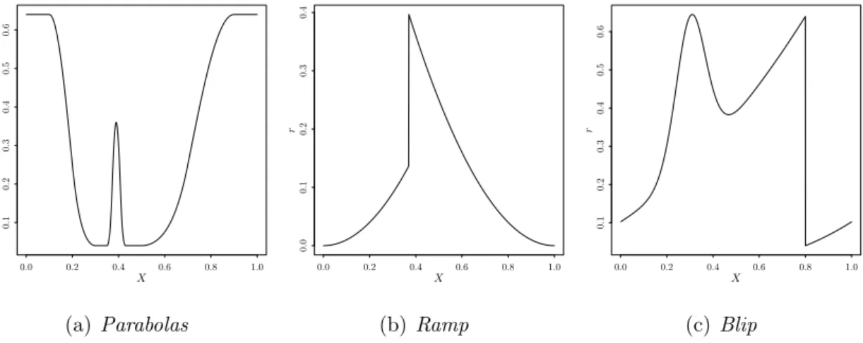
0.0 0.2 0.4 0.6 0.8 1.0 0.1 0.2 0.3 0.4 0.5 0.6 X r (a)Parabolas 0.0 0.2 0.4 0.6 0.8 1.0 0.0 0.1 0.2 0.3 0.4 X r (b) Ramp 0.0 0.2 0.4 0.6 0.8 1.0 0.1 0.2 0.3 0.4 0.5 0.6 X r (c) Blip
Figure 1: The three test functions considered.
findings using numerical examples. We begin by giving some details about the speci-ficities inherent in wavelet estimators in a non-deterministic design framework. We also try to propose a realistic simulation setting using an adaptive selection method to select both the truncation parameter of the linear estimator and the threshold parameter of the non-linear estimator. In this context, we compare their empirical performances in the model with both multiplicative and additive noise. Simulations were performed usingRand in particular therwaveletpackageNavarro and Chesneau(2019) (available fromhttps://github.com/fabnavarro/rwavelet).
4.1
Computational aspect of wavelets and parameters
selec-tion
For fixed design, thanks to Mallat’s pyramidal algorithm (Mallat,2008), the computa-tion of wavelet-based estimators is simple and fast. When considering uniform random design, the implementation requires some changes and several strategies have been de-veloped in the literature (see, e.g., Cai et al. (1998); Hall et al. (1997)). For uniform design regression, Cai and Brown (1999) has proposed to use an approach in which the wavelet coefficients are computed by a simple application of Mallat’s algorithm using the orderedYi’s as input variables. We have followed this approach because it preserves
the simplicity of calculation and the efficiency of the equispaced algorithm. In the context of wavelet regression in random design with heteroscedastic noise, Kulik et al.
(2009) and Navarro and Saumard (2017) also adopted this approach.
to select the threshold parameter in wavelet shrinkage (see,Nason(1996)). For the cal-ibration of linear wavelet estimators, his strategy was used by Navarro and Saumard
(2017). We have chosen to apply this approach to select both the threshold and trun-cation parameter of linear and non-linear estimators. More precisely, in the linear case, we built a collection of linear estimators ˆrlin
j∗,n, j∗ = 0,1, . . . ,log 2(n)−1 (by successively adding whole resolution levels of wavelet coefficients), and select the best among this collection by minimizing a 2FCV criterion denoted by 2FCV(j∗). The resulting
esti-mator of the truncation level is denoted by ˆj∗ and the corresponding estimator of r
by ˆrlin ˆ
j∗,n (see, Navarro and Saumard (2017, 2018) for more details). For the nonlinear estimator, the same estimator ˆj∗ of the truncation parameter j∗ obtained for the
lin-ear is used. The estimator of the thresholding parameter is obtained using the 2FCV method developed in Nason (1996). The parameter j1 is fixed a priori as the
maxi-mum level allowed by the wavelet decomposition (i.e.,j1 = log 2(n)−1). It is a classic
choice that allows the coefficients to be selected down to the smallest scale. In addi-tion, in order to facilitate and not to overburden the implementation of the nonlinear estimator, we perform a standard hard thresholding of the wavelet coefficient estima-tors (rather than the double threshold used in its definition). In order to be able to evaluate the performance of these two criteria, the mean square error (MSE) is used (i.e., MSE(ˆrj∗,n, r) =
1
n
Pn
i=1(r(Xi)−ˆrj∗,n(Xi))
2)). We consider three test functions for r (see Figure 1), commonly used in the wavelet literature, Parabolas, Ramp and Blip
(see, e.g., Donoho et al. (1995)). In all simulations, we examine the case d = 1, the design is chosen to satisfyA.2(i.e.,U([0,1])) and the choice of the wavelet family used is also fixed (i.e., Daubechies compactly supported wavelet with 8 vanishing moments).
4.2
Additive-multiplicative regression
This subsection examines the behaviour and performance of linear and non-linear es-timators in the context of additive and multiplicative regression by considering V1 ∼
N(0, σ2), where σ2 = 0.01 and U1 ∼ U([−1,1]). Thus, the goal is to estimate the
frontier r from (Xi, Yi) sample simulated from one of the test functions. By applying
one of the linear or nonlinear methods developed above to the estimation ofr, one can construct an estimator whose rate of convergence is given by (5a) and (5b) respectively.
Note that here, the nature of the frontier function is not necessarily the same as that commonly found in the literature on stochastic boundary estimation. Indeed, here r
is not necessarily a production function (e.g., r is concave), the only assumption we make is given by A.1. Thus, the application here can be seen as the estimation of the boundary or frontier of a sample affected by some additive (positive) noise (see Jirak
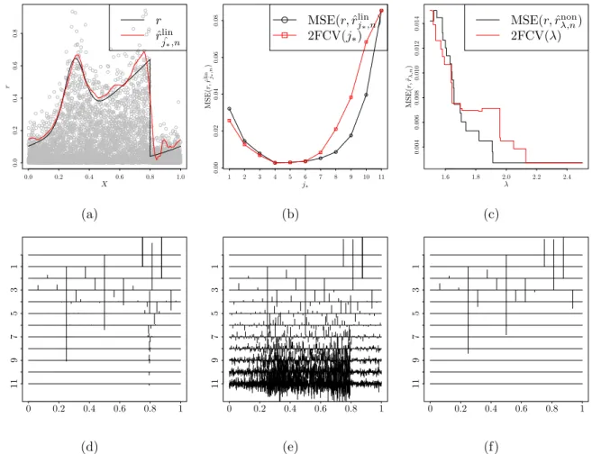
et al. (2014)). 0.0 0.2 0.4 0.6 0.8 1.0 0.0 0.2 0.4 0.6 0.8 X r r ˆ rlin ˆ j∗,n (a) 1 2 3 4 5 6 7 8 9 10 11 0.00 0.02 0.04 0.06 0.08 j∗ MSE( r, ˆ r linj,n∗ ) MSE(r,rˆlin j∗,n) 2FCV(j∗) (b) 1.6 1.8 2.0 2.2 2.4 0.004 0.006 0.008 0.010 0.012 0.014 λ MSE( r, ˆ rλ,n ) MSE(r,ˆrnon λ,n) 2FCV(λ) (c) 11 9 7 5 3 1 0 0.2 0.4 0.6 0.8 1 (d) 11 9 7 5 3 1 0 0.2 0.4 0.6 0.8 1 (e) 11 9 7 5 3 1 0 0.2 0.4 0.6 0.8 1 (f)
Figure 2: Typical estimation from a single simulation forn = 4096 andσ2 = 0.01. Noisy observations (X, Y2) (grey circles), true function (black line) and ˆrlin
ˆj∗,n (a). Graphs of
the MSE (black line) againstj∗and (rescaled) 2FCV(·) criterion (red line) for the linear
(b) and nonlinear (c) cases respectively. Original wavelet coefficients (d). Noisy wavelet coefficients (e). Estimated wavelet coefficients (f).
A typical example of estimation for the Blip function, with n = 4096 is given in Figure2. It can be seen that the minimum of 2FCV(j∗) criteria coincides with that of
unknown risk (i.e., ˆj∗ = 4) and therefore provides the best possible linear estimator for
the collection under consideration (i.e., MSE(r,ˆrˆlinj
0.003 0.006 0.009 0.012
2FCVlin2FCVnon MSElin MSEnon
MSE (a) Parabolas 0.001 0.002 0.003 0.004
2FCVlin2FCVnon MSElin MSEnon
MSE (b) Ramp 0.0025 0.0050 0.0075 0.0100
2FCVlin2FCVnon MSElin MSEnon
MSE
(c) Blip
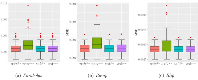
Figure 3: Box plots of the MSE for the three-test functions withn = 4096 andσ2 = 0.01.
the results of the non-linear estimator in Figure2. Indeed, in this case, the value of the threshold obtained by minimizing the cross validated criterion leads to the elimination of all the thresholded coefficients (i.e., going from ˆj∗ to j1) and therefore leads to the
same estimate and the same risk as the linear estimator. We can see (Figure2(c)) that the unknown risk behaves in the same way here. This is partly because the amplitude of the coefficients at the fine scales is so large and variable from one scale to another that it is not possible to obtain an overall optimal threshold value that makes it possible to maintain certain important coefficients and that, on the contrary, keeps coefficients associated with noise, with this specific thresholding policy (i.e., a ‘keep’ or ‘kill’ rule). In particular the important coefficients located on scales larger than ˆj∗ (especially those
encoding the discontinuity ofr) are too small in amplitude to be maintained by a global threshold.
In order to determine whether this phenomenon observed for a single function and a single realization is confirmed in a more general context, we compare the performance in terms of MSE (computed on the functions after reconstruction) for both estimators and for the three-test functions. For each function, a sample of N = 100 is generated and we compare the average behavior of the MSE for parameters selected with the oracle obtained by minimizing the MSE using the original signalr (denoted by MSElin and MSEnonrespectively), the linear 2FCVlin strategy and the non-linear 2FCVnon (i.e., calculated from ˆj∗ and the threshold that minimizes the 2FCV(λ)) strategy. Figure 3
presents the results in the form of boxplots, one for each function. On the one hand, for all three functions, we can see that the performance of 2FCVlin is at the MSElin
0.005 0.010
2FCVlin2FCVnon MSElin MSEnon
MSE (a) Parabolas 0.001 0.002 0.003 0.004
2FCVlin2FCVnon MSElin MSEnon
MSE
(b) Ramp
0.016 0.020 0.024
2FCVlin2FCVnon MSElin MSEnon
MSE
(c) Blip
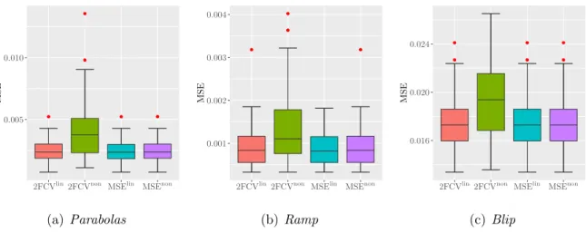
Figure 4: Box plots of the MSE for the three-test functions with n = 2048 and σ2 =
0.025.
level. This procedure therefore provides a remarkable surrogate of the unknown risk. On the other hand, the non-linear 2FCVnon oracle is similar to MSElin, which means that the optimal threshold here leads systematically to the suppression of all threshold coefficients — which corresponds to the selection of values of the threshold parameter which is greater than the largest noisy wavelet coefficient in absolute value. Finally, the variability of the 2FCVnon is high as a result of selected threshold values that are sometimes too small, resulting in the conservation of unnecessary coefficients in the reconstruction. This is because the curves associated with non-linear criteria do not generally allow a single global minimum, but the minimum is reached in the form of a plateau (see Figure 2(c)). In practice, when the minimum is reached on such a plateau, the first element that constitutes it is selected first. This has no influence on MSEnon but generates this variability of 2FCVnon, i.e., when the abscissa of the first point constituting the plateau associated with 2FCVnon is lower than that of MSEnon) Note that to overcome this problem, in the presence of a plateau, we could for example select a threshold value in the middle of it. We have not done so here to emphasize the fact that a cross validation strategy of the global threshold seems ineffective in this setting. It should also be noted that in our simulations, this finding is also verified for other noise levels or sample sizes (the results are generally very similar, so we give only another example by considering a lower number of samples,n= 2048 and a lower additive noise level σ2 = 0.025).
ap-proach in the context of the simulations considered in this study. One way to fully benefit from the non-linear approach would be to consider an optimal threshold selec-tion strategy on a scale by scale basis. The selecselec-tion procedure used here, based on an interpolation performed in the original domain, does not facilitate this extension. For this purpose it would be necessary, for example, to define an interpolated version of the cross validation method in the wavelet coefficients domain.
5
Auxiliary results and proof of the main result
5.1
Auxiliary results
In this section, we provide some lemmas for the proof of the main Theorem.
Lemma 5.1. Let j ≥τ, k∈Λj, αˆj,k be (3). Then, under H.1 or H.2, we have
E[ ˆαj,k] =αj,k, E " 1 n n X i=1 Yi2Ψj,k,u(Xi)−wj,k,u # =βj,k,u.
Proof of Lemma 5.1. Using the independence assumptions on the random variables, H.1 or H.2, observe that E[U1V1f(X1)Φj,k(X1)] = E[U1]E[V1]E[f(X1)Φj,k(X1)] under A.5, E[U1]E[V1f(X1)Φj,k(X1)] under A.6, = 0, and vj,k= E[V2 1] 2 −jd/2 =E[V2 1] R [0,1]dΦj,k(x)dx=E[V12]E[Φj,k(X1)] under A.5, Z [0,1]d g2(x)Φj,k(x)dx under A.6, =EV12Φj,k(X1) . Therefore E[ ˆαj,k] =E " 1 n n X i=1 Yi2Φj,k(Xi)−vj,k # =EY12Φj,k(X1) −vj,k =EU12r(X1)Φj,k(X1) + 2E[U1V1f(X1)Φj,k(X1)] +E V12Φj,k(X1) −vj,k =EU12E[r(X1)Φj,k(X1)] = Z [0,1]d r(x)Φj,k(x)dx=αj,k.
Using similar mathematical arguments, sinceR[0,1]dΨj,k,u(x)dx= 0, we have wj,k,u = 0 = EV12 Z [0,1]d Ψj,k,u(x)dx=E V12E[Ψj,k,u(X1)] under A.5, Z [0,1]d g2(x)Ψj,k,u(x)dx under A.6, =EV12Ψj,k,u(X1) .
We prove the second equality. The proof of Lemma 5.1 is complete.
Lemma 5.2. Let j ≥ τ such that 2j ≤ n, k ∈ Λ
j, αˆj,k and βˆj,k,u be (3) and (4)
respectively. Then, under H.1 or H.2,
E( ˆαj,k−αj,k)2 . 1 n, E h ( ˆβj,k,u−βj,k,u)2 i . lnn n .
Proof of Lemma 5.2. Owing to Lemma 5.1 we have E[ ˆαj,k] =αj,k. Therefore
E ( ˆαj,k−αj,k)2 =V[ ˆαj,k] =V " 1 n n X i=1 Yi2Φj,k(Xi)−vj,k # =V " 1 n n X i=1 Yi2Φj,k(Xi) # = 1 nV Y12Φj,k(X1) ≤ 1 nE Y14Φ2j,k(X1) . 1 n E U14f4(X1)Φ2j,k(X1) +EV14Φ2j,k(X1) = 1 n E U14Ef4(X1)Φ2j,k(X1) +EV14Φ2j,k(X1) . (6) ByA.1and EΦ2j,k(X1) =R[0,1]d(Φj,k(x)) 2 dx= 1, we haveEf4(X1)Φ2j,k(X1) .1. On the other hand, we have
EV14Φ2j,k(X1) = EV14EΦ2j,k(X1) .1 under A.5, Z [0,1]d g4(x)Φ2j,k(x)dx. Z [0,1]d Φ2j,k(x)dx= 1 under A.6.
Thus all the terms in the brackets of (6) are bounded from above. The first inequality in Lemma 5.2 is proved.
Now, by the definition of ˆβj,k,u, taking Ki := Yi2Ψj,k,u(Xi) −wj,k,u and Di :=
Ki1{|Ki|≤ρn}−E
Ki1{|Ki|≤ρn}
for the sake of simplicity, the second equation in Lemma
5.1 yields ˆ βj,k,u−βj,k,u= 1 n n X i=1 Di−E K11{|K1|>ρn} .
Hence, using E " (1/n) n P i=1 Di 2# = (1/n2)V n P i=1 Di = V[D1]/n ≤ E[D21]/n, we have Eh( ˆβj,k,u−βj,k,u)2 i .E 1 n n X i=1 Di !2 + E |K1|1{|K1|>ρn} 2 . . 1 nE D12+ E|K1|1{|K1|>ρn} 2 .
Proceeding as for the proof of the first inequality, using the assumptions H.1 or H.2, note that E[K2 1].E Y4 1Ψ2j,k,u(X1) +w2 j,k,u .1 and EK11{|K1|>ρn} 2 . EK12/ρn 2 . lnn n . (7) Therefore, E h ( ˆβj,k,u−βj,k,u)2 i . 1 n + lnn n . lnn n .
The second inequality in Lemma5.2 is proved. This ends the proof of Lemma 5.2.
Lemma 5.3. Let j ≥τ such that 2jd .n/lnn, k∈Λ
j, βˆj,k,u be (4). Then there exists
a constant κ >1 such that
P(|βˆj,k,u−βj,k,u| ≥κtn).n−4.
Proof of Lemma 5.3. By the definition of ˆβj,k,u, taking Ki :=Yi2Ψj,k,u(Xi)−wj,k,u
andDi :=Ki1{|Ki|≤ρn}−E
Ki1{|Ki|≤ρn}
for the sake of simplicity, the second equation in Lemma 5.1 yields |βˆj,k,u−βj,k,u|. 1 n n X i=1 Di +E|K1|1{|K1|>ρn} .
Using (7), there exists c >0 such that E|K1|1{|K1|>ρn}
≤cplnn/n. Then {|βˆj,k,u−βj,k,u| ≥κtn} ⊆ ( 1 n n X i=1 Di ≥(κ−c)tn ) .
Note that E[Di] = 0 thanks to Lemma 5.1. According to the proof of Lemma 5.2,
E[D2
i] :=δ2 .1. This with|Di|.
p
n/lnn and Bernstein inequality shows
P 1 n n X i=1 Di ≥(κ−c)tn ! .exp − n(κ−c) 2t2 n 2(δ2+ (κ−c)t nρn/3) .exp −lnn (κ−c) 2 2(δ2+ (κ−c)/3) .n− (κ−c)2 2(δ2+(κ−c)/3).
Then one choose large enough κ such that
P(|βˆj,k,u−βj,k,u| ≥κtn).n
−2(δ2+(κ(κ−1)2
−1)/3) .n−4.
This is the desired conclusion.
5.2
Proof of the main result
This section is devoted to the proof of Theorem3.1. We prove (5a) and (5b) in turn.
Proof of (5a) Note that
E Z [0,1]d ˆrnlin(x)−r(x) 2 dx =Ehrˆlinn −Pj∗r 2 2 i +Pj∗r−r 2 2. (8)
It is easy to see that
Ehrˆlinn −Pj∗r 2 2 i =E X k∈Λj∗ ( ˆαj∗,k−αj∗,k)Φj∗,k 2 2 = X k∈Λj∗ E αˆj∗,k−αj∗,k 2 . According to Lemma5.2, |Λj∗|∼2 j∗d and 2j∗ ∼n 1 2s0+d, Ehˆrlinn −Pj∗r 2 2 i . 2 j∗d n ∼n − 2s0 2s0+d. (9)
When p≥2,s0 =s. By H¨older inequality andr ∈Bp,qs ([0,1]d),
kPj∗r−rk 2 2 .kPj∗r−rk 2 p .2 −2j∗s ∼n− 2s 2s+d. When 1≤p <2 and s > d/p,Bs p,q([0,1]d)⊆Bs 0 2,∞([0,1]d) kPj∗r−rk 2 2 . ∞ X j=j∗ 2−2js0 .2−2j∗s0 ∼n− 2s0 2s0+d.
Therefore, in both cases,
kPj∗r−rk 2 2 .n − 2s0 2s0+d. (10) By (8), (9) and (10), E Z [0,1]d rˆlinn (x)−r(x) 2 dx .n− 2s 0 2s0+d.
Proof of (5b) We now follow the lines of (Delyon and Juditsky,1996, Theorem 2) with adaptation to our statistical setting, by using the definitions of our estimators and the
auxiliary results of Section5.1. By the definitions of ˆrlin
n and ˆrnnon, we have
ˆ rnnon(x)−r(x) =rˆlinn (x)−Pj∗r(x) −r(x)−Pj1+1r(x) + j1 X j=j∗ 2d−1 X u=1 X k∈Λj ˆ βj,k,u1{|βj,ˆ k,u|≥κtn}−βj,k,u Ψj,k,u(x). Hence, E Z [0,1]d rˆ non n (x)−r(x) 2 dx .T1+T2+Q, where T1 :=E rˆ lin n −Pj∗r 2 2 , T2 := r−Pj1+1r 2 2 and Q:=E j1 X j=j∗ 2d−1 X u=1 X k∈Λj ˆ βj,k,u1{|βj,ˆ k,u|≥κtn}−βj,k,u Ψj,k,u 2 2 . According to (9) and 2j∗ ∼n2m+d1 (m > s), T1 =E rˆ lin n −Pj∗r 2 2 . 2 j∗d n ∼n −2m+d2m < n−2s+d2s .
When p ≥2, by the same arguments as (10) shows T2 = r−Pj1+1r 2 2 . 2 −2j1s. This with 2j1 ∼(n/lnn)d1 leads to T2 .2−2j1s ∼ lnn n 2sd ≤(lnn)n−2s+d2s .
On the other hand, Bs
p,q([0,1]d) ⊆ B s+d/2−d/p 2,∞ ([0,1]d) when 1 ≤ p < 2 and s > d/p. Then T2 .2 −2j1(s+d2−d p) ∼ lnn n 2(s+d 2−dp) d ≤(lnn)n−2s+d2s . Hence, T2 .(lnn)n− 2s 2s+d, for each 1≤p <+∞.
The main work for the proof of (5b) is to show
Q=E j1 X j=j∗ 2d−1 X u=1 X k∈Λj ˆ βj,k,u1{|βˆj,k,u|≥κtn}−βj,k,u Ψj,k,u 2 2 .(lnn)n −2s+d2s . Note that Q= j1 X j=j∗ 2d−1 X u=1 X k∈Λj E ˆ βj,k,u1{|βj,ˆ k,u|≥κtn}−βj,k,u 2 .Q1+Q2+Q3, (11)
where Q1 = j1 X j=j∗ 2d−1 X u=1 X k∈Λj E ˆ βj,k,u−βj,k,u 2 1{|βj,ˆ k,u−βj,k,u|>κtn2 } , Q2 = j1 X j=j∗ 2d−1 X u=1 X k∈Λj E ˆ βj,k,u−βj,k,u 2 1{|βj,k,u|≥κtn2 } , Q3 = j1 X j=j∗ 2d−1 X u=1 X k∈Λj |βj,k,u| 21 {|βj,k,u|≤2κtn}.
ForQ1, one observes that
E ˆ βj,k,u−βj,k,u 2 1{|βj,ˆ k,u−βj,k,u|>κtn2 } ≤ E ˆ βj,k,u−βj,k,u 412 P |βˆj,k,u−βj,k,u|> κtn 2 12
thanks to H¨older inequality. By Lemma 5.2, Lemma 5.3 and |βˆj,k,u−βj,k,u|2 .n/lnn,
E ˆ βj,k,u−βj,k,u 2 1{|βj,ˆ k,u−βj,k,u|>κtn2 } . 1 n2. Then Q1 . j1 P j=j∗
2jd/n2 . 2j1d/n2 . 1/n ≤ n−2s+d2s , where one uses the choice 2j1 ∼
(n/lnn)1d. Hence,
Q1 ≤n−
2s
2s+d. (12)
To estimate Q2, one defines
2j0 ∼n2s+d1 .
It is easy to see that 2j∗ ∼n2m+d1 ≤2j0 ∼ n 1 2s+d ≤ 2j1 ∼ (n/lnn)1d. Furthermore, one rewrites Q2 = j0 X j=j∗ + j1 X j=j0+1 ! 2d−1 X u=1 X k∈Λj E ˆ βj,k,u−βj,k,u 2 1{|βj,k,u|≥κtn2 } :=Q21+Q22. By Lemma 5.2 and 2j0 ∼n2s+d1 , Q21:= j0 X j=j∗ 2d−1 X u=1 X k∈Λj E ˆ βj,k,u−βj,k,u 2 1{|βj,k,u|≥κtn2 } . j0 X j=j∗ 2d−1 X u=1 X k∈Λj lnn n . j0 X j=j∗ (lnn)2 jd n .(lnn) 2j0d n ∼(lnn)n − 2s 2s+d.
On the other hand, it follows from Lemma5.2 that Q22:= j1 X j=j0+1 2d−1 X u=1 X k∈Λj E ˆ βj,k,u−βj,k,u 2 1{|βj,k,u|≥κtn2 } . j1 X j=j0+1 2d−1 X u=1 X k∈Λj lnn n 1{|βj,k,u|≥κtn2 }.
When p≥2, sincer ∈Bp,qs ([0,1]d), Lemma 5.2 and tn=
p lnn/n, Q22 . j1 X j=j0+1 2d−1 X u=1 X k∈Λj lnn n 1{|βj,k,u|≥κtn2 } . j1 X j=j0+1 2d−1 X u=1 X k∈Λj lnn n βj,k,u κtn/2 2 . j1 X j=j0+1 2−2js.2−2j0s∼n−2s+d2s . (13) When 1≤p <2 and s > d/p,Bs p,q([0,1]d)⊆B s+d/2−d/p 2,∞ ([0,1]d). Then Q22 . j1 X j=j0+1 2d−1 X u=1 X k∈Λj lnn n 1{|βj,k,u|≥κtn2 } . j1 X j=j0+1 2d−1 X u=1 X k∈Λj lnn n βj,k,u κtn/2 p . j1 X j=j0+1 (lnn)np2−12−j(s+d/2−d/p)p .(lnn)np2−12−j 0(s+d/2−d/p)p ∼(lnn)n− 2s 2s+d. (14)
It follows from the upper bounds above that
Q2 .(lnn)n−
2s
2s+d. (15)
Finally, one evaluates Q3. Clearly,
Q31 := j0 X j=j∗ 2d−1 X u=1 X k∈Λj |βj,k,u| 21 {|βj,k,u|≤2κtn} ≤ j0 X j=j∗ 2d−1 X u=1 X k∈Λj 2κtn 2 . j0 X j=j∗ lnn n 2 jd . lnn n 2 j0d.
This with the choice of 2j0 shows
Q31.(lnn)n−
2s 2s+d.
On the other hand, Q32 :=
j1 P j=j0+1 2d−1 P u=1 P k∈Λj
|βj,k,u|21{|βj,k,u|≤2κtn}. According to the
argu-ments of (13), forp≥2, Q32. j1 X j=j0+1 2d−1 X u=1 X k∈Λj |βj,k,u| 2 .n−2s+d2s .
When 1 ≤ p <2, |βj,k,u| 21 {|βj,k,u|≤2κtn} ≤ |βj,k,u| p |2κtn| 2−p
. Then similar to the argu-ments of (14), Q32 . j1 X j=j0+1 2d−1 X u=1 X k∈Λj |βj,k,u|p|2κtn|2 −p . lnn n 2−2p j1 X j=j0+1 2−j(s+d/2−d/p)p . lnn n 2−2p 2−j0(s+d/2−d/p)p . lnn n 2−2p 1 n (s+d/22s+d−d/p)p ≤(lnn)n−2s+d2s .
It follows from the inequalities above that
Q3 .(lnn)n−
2s
2s+d, (16)
in both cases. Owing to (11), (12), (15), and (16), we prove that
Q.(lnn)n−2s+d2s ,
which is the desired conclusion.
Acknowledgements
We would like to thank the reviewers for their thoughtful comments that have improved the manuscript.
References
Abramovich, F., T. C. Bailey, and T. Sapatinas (2000). Wavelet analysis and its sta-tistical applications. Journal of the Royal Statistical Society: Series D (The Statisti-cian) 49(1), 1–29.
Brown, L. D., M. Levine, et al. (2007). Variance estimation in nonparametric regression via the difference sequence method. The Annals of Statistics 35(5), 2219–2232.
Cai, T. T. and L. D. Brown (1999). Wavelet estimation for samples with random uniform design. Statistics & Probability Letters 42(3), 313–321.
Cai, T. T., L. D. Brown, et al. (1998). Wavelet shrinkage for nonequispaced samples.
The Annals of Statistics 26(5), 1783–1799.
Cai, T. T., L. Wang, et al. (2008). Adaptive variance function estimation in het-eroscedastic nonparametric regression. The Annals of Statistics 36(5), 2025–2054.
Chaubey, Y. P., C. Chesneau, and H. Doosti (2015). Adaptive wavelet estimation of a density from mixtures under multiplicative censoring. Statistics 49(3), 638–659.
Chesneau, C. (2013). On the adaptive wavelet estimation of a multidimensional regres-sion function under α-mixing dependence: Beyond the standard assumptions on the noise. Commentationes Mathematicae Universitatis Carolinae 4, 527–556.
Chesneau, C., J. Kou, and F. Navarro (2019). Linear wavelet estimation in regression with additive and multiplicative noise. working paper or preprint.
Chichignoud, M. (2012). Minimax and minimax adaptive estimation in multiplicative regression: locally bayesian approach. Probability Theory and Related Fields 153 (3-4), 543–586.
Cohen, A., I. Daubechies, and P. Vial (1993). Wavelets on the interval and fast wavelet transforms. Applied and Computational Harmonic Analysis 1(1), 54–81.
Comte, F. (2015). Estimation non-param´etrique. Spartacus-IDH.
Daouia, A. and L. Simar (2005). Robust nonparametric estimators of monotone bound-aries. Journal of Multivariate Analysis 96(2), 311–331.
Daubechies, I. (1992). Ten lectures on wavelets, Volume 61. Siam.
De Prins, D., L. Simar, and H. Tulkens (1984). Measuring labour efficiency.Post Offices in The Performance of Public Enterprises: Concepts and Measurement (P. Pestieau
ve H. Tulkens M. Marchand), 243–267.
Delyon, B. and A. Juditsky (1996). On minimax wavelet estimators. Applied and Computational Harmonic Analysis 3(3), 215–228.
Donoho, D. L., I. M. Johnstone, G. Kerkyacharian, and D. Picard (1995). Wavelet shrinkage: asymptopia? Journal of the Royal Statistical Society. Series B (Method-ological), 301–369.
Fan, Y., Q. Li, and A. Weersink (1996). Semiparametric estimation of stochastic pro-duction frontier models. Journal of Business & Economic Statistics 14(4), 460–468.
Farrell, M. J. (1957). The measurement of productive efficiency. Journal of the Royal Statistical Society: Series A (General) 120(3), 253–281.
Gijbels, I., E. Mammen, B. U. Park, and L. Simar (1999). On estimation of mono-tone and concave frontier functions. Journal of the American Statistical Associa-tion 94(445), 220–228.
Girard, S., A. Guillou, and G. Stupfler (2013). Frontier estimation with kernel regression on high order moments. Journal of Multivariate Analysis 116, 172–189.
Girard, S. and P. Jacob (2008). Frontier estimation via kernel regression on high power-transformed data. Journal of Multivariate Analysis 99(3), 403–420.
Hall, P. and J. Marron (1990). On variance estimation in nonparametric regression.
Biometrika 77(2), 415–419.
Hall, P., B. A. Turlach, et al. (1997). Interpolation methods for nonlinear wavelet regression with irregularly spaced design. The Annals of Statistics 25(5), 1912–1925.
H¨ardle, W., G. Kerkyacharian, D. Picard, and A. Tsybakov (2012). Wavelets, ap-proximation, and statistical applications, Volume 129. Springer Science & Business Media.
H¨ardle, W. and A. Tsybakov (1997). Local polynomial estimators of the volatility function in nonparametric autoregression. Journal of Econometrics 81(1), 223–242.
Huang, P., Y. Pi, and I. Progri (2013). Gps signal detection under multiplicative and additive noise. The Journal of Navigation 66(4), 479–500.
Jirak, M., A. Meister, M. Reiß, et al. (2014). Adaptive function estimation in nonpara-metric regression with one-sided errors. The Annals of Statistics 42(5), 1970–2002.
Korostelev, A. P. and A. B. Tsybakov (2012). Minimax theory of image reconstruction, Volume 82. Springer Science & Business Media.
Kuan, D. T., A. A. Sawchuk, T. C. Strand, and P. Chavel (1985). Adaptive noise smoothing filter for images with signal-dependent noise. IEEE Transactions on Pat-tern Analysis & Machine Intelligence (2), 165–177.
Kulik, R., M. Raimondo, et al. (2009). Wavelet regression in random design with heteroscedastic dependent errors. The Annals of Statistics 37(6A), 3396–3430.
Kulik, R., C. Wichelhaus, et al. (2011). Nonparametric conditional variance and er-ror density estimation in regression models with dependent erer-rors and predictors.
Electronic Journal of Statistics 5, 856–898.
Kumbhakar, S. C., B. U. Park, L. Simar, and E. G. Tsionas (2007). Nonparametric stochastic frontiers: a local maximum likelihood approach. Journal of Economet-rics 137(1), 1–27.
Mallat, S. (2008). A wavelet tour of signal processing: the sparse way. Academic press.
Mateo, J. L. and A. Fern´andez-Caballero (2009). Finding out general tendencies in speckle noise reduction in ultrasound images.Expert Systems with Applications 36(4), 7786–7797.
Meyer, Y. (1992). Wavelets and operators, Volume 1. Cambridge university press.
Muller, H.-G., U. Stadtmuller, et al. (1987). Estimation of heteroscedasticity in regres-sion analysis. The Annals of Statistics 15(2), 610–625.
Nason, G. P. (1996). Wavelet shrinkage using cross-validation. Journal of the Royal Statistical Society. Series B (Methodological), 463–479.
Navarro, F. and C. Chesneau (2019). R package rwavelet: Wavelet Analysis. (Version 0.4.0).
Navarro, F. and A. Saumard (2017). Slope heuristics and v-fold model selection in heteroscedastic regression using strongly localized bases. ESAIM: Probability and Statistics 21, 412–451.
Navarro, F. and A. Saumard (2018). Efficiency of the v -fold model selection for local-ized bases. In P. Bertail, D. Blanke, P.-A. Cornillon, and E. Matzner-Løber (Eds.),
Nonparametric Statistics, Cham, pp. 53–68. Springer International Publishing.
Rabbani, H., M. Vafadust, P. Abolmaesumi, and S. Gazor (2008). Speckle noise reduc-tion of medical ultrasound images in complex wavelet domain using mixture priors.
IEEE Transactions on Biomedical Engineering 55(9), 2152–2160.
Shen, Y., C. Gao, D. Witten, and F. Han (2019). Optimal estimation of variance in nonparametric regression with random design. arXiv preprint arXiv:1902.10822.
Simar, L. and V. Zelenyuk (2011). Stochastic fdh/dea estimators for frontier analysis.
Journal of Productivity Analysis 36(1), 1–20.
Triebel, H. (1994). Theory of function spaces ii. Bull. Amer. Math. Soc 31, 119–125.
Tsybakov, A. B. (2009). Introduction to nonparametric estimation. revised and ex-tended from the 2004 french original. translated by vladimir zaiats.
Verzelen, N., E. Gassiat, et al. (2018). Adaptive estimation of high-dimensional signal-to-noise ratios. Bernoulli 24(4B), 3683–3710.
Wang, L., L. D. Brown, T. T. Cai, M. Levine, et al. (2008). Effect of mean on variance function estimation in nonparametric regression. The Annals of Statistics 36(2), 646–664.