MPRA
Munich Personal RePEc Archive
A Time Series Approach to the
Feldstein-Horioka Puzzle with Panel
Data from the OECD Countries
Saten Kumar and B. Bhaskara Rao
Auckland University of Technology, University of Western Sydney
8. November 2009
Online at
http://mpra.ub.uni-muenchen.de/18464/
A Time Series Approach to the Feldstein-Horioka Puzzle with Panel Data from the OECD Countries
Saten Kumar
kumar_saten@yahoo.com
Auckland University of Technology, Auckland (New Zealand)
B. Bhaskara Rao
raob123@bigpond.com
University of Western Sydney, Sydney (Australia)
Abstract
The Pedroni method is used to estimate the Feldstein-Horioka equation from 1960-2007 with a panel of 13 OECD countries. It is found that the Feldstein-Horioka puzzle exists in a weaker form with a much reduced saving retention coefficient. The Bretton Woods agreement in particular has weakened the Feldstein-Horioka puzzle by significantly
improving the international capital mobility. In comparison the Maastricht agreement seems to have improved capital mobility only by a small magnitude. The structural break tests of Westerlund are used in this paper.
Keywords: Feldstein-Horioka puzzle, Structural breaks, Bretton Woods and Maastricht agreements and International capital mobility.
1. Introduction
The high correlation between domestic savings and investment is well known as the
Feldstein-Horioka puzzle (henceforth FHP). It has started with Feldstein and Horioka (1980, henceforth FH) where they have shown with the cross-section data of 16 OECD countries for the period 1960-1974, that investment and saving ratios are highly correlated. Therefore, they argued that domestic saving is the main source of funds for investment, which in turn,
according to them implies that international capital mobility is low. However, this implication as evidence against capital mobility was questioned by some authors. Jensen (1996, 1998), Coakley and Kulasi (1997) and Pelgrin and Schich (2004) interpret the close long run relationship between the investment and saving ratios as a solvency condition that must be satisfied and not as evidence against international capital mobility. Nevertheless, we take the view that the FHP is a simple and indirect test on the extent to which capital is mobile across the countries and if tested for structural breaks it can also give an indication about changes in capital mobility. Capital mobility, in its own right, is important because it has implications for single currency debates, tax policies on capital and saving, whether growth is constrained by domestic saving and for the crowding effects of fiscal deficits. On the other hand if capital mobility is high, countries cannot pursue independent monetary policies. Because of these policy implications Obstfeld and Rogoff (2000) have called FHP the mother of all puzzles.
In the FH cross section regressions of the ratio of investment to GDP (investment ratio) on the ratio of saving to GDP (saving ratio), the coefficient of the saving ratio, known as the saving retention coefficient (β), was almost unity. This puzzle, in spite of a number of empirical investigations with alternative data sets, specifications and estimation technique, still remains a puzzle. The vast empirical literature on FHP is comprehensively surveyed by Apergis and Tsoumas (2009). They conclude that the majority of the empirical studies do not support the original strong results of FH but found that this correlation still exists in a weaker form in that βseems to have decreased and significantly less than unity.
The outline of this paper is as follows. Section 2 briefly reviews a few relevant empirical works. In Section 3 empirical results for panel unit root and cointegration tests and estimates of the cointegrating equations with tests for structural breaks are presented. Section 4 concludes.
2. Brief Overview of Panel Studies on FHP
To test the validity of FHP many studies have estimated the following equation or its variants:1
+ (1)
it i i it it
ITY =
α
+β
STYε
where ITY is the domestic investment share of GDP and STY is the domestic saving share of GDP, andi tare country and time subscripts and
ε
it ∼N
(0, ) for all and .σ
i t A few recent panel data studies on FHP are Coakley et al. (1999, 2001 and 2004), Cadoret (2001),Giannone and Lenza (2004), Pelgrin and Schich (2004), Bahmani-Oskooee and Chakrabarti (2005), Kim et al. (2005), Chakrabarti (2006), Murthy (2007), Christopoulos (2007), Di Iorio and Fachin (2007), Herwartz and Xu (2009) and Fouquau et al. (2009).2 The results in these studies differ considerably with some supporting and some against the validity of FHP.3
1
The null hypothesis is that, under complete capital mobility β in equation (1) should be zero. FH interpret this coefficient, also called saving retention coefficient, as an indicator of the degree of international capital
mobility. Their empirical findings show that β is very close to one (between 0.85 to 0.95), indicating low capital mobility in the sample OECD countries.
2
For discussions on cross-section and time series studies on FHP, see Apergis and Tsoumas (2009). For our purpose, we review only key empirical studies that utilise panel data estimation methods to examine the FH hypothesis.
3
Di Iorio and Fachin (2007) employed the panel bootstrap tests to examine the FHP for a panel of 12 EU countries over the period 1960-2002. Their country specific Fully Modified Ordinary Least Squares (FMOLS) estimates of βrange from 0.59 to 1.03. Christopoulos (2007) used the panel Dynamic Ordinary Least Squares (DOLS) to examine the FHP for 13 OECD countries. The estimate ofβis around 0.5 for whole sample period (1885–1992). However, for sub-sample periods (pre-Maastricht periods ie, 1921-1992 and 1950-1992) the estimated values of β ranged from 0.79 and 0.90, respectively. Murthy (2007) used the maximum likelihood panel cointegration techniques to examine the validity of FHP for fourteen Latin American and four Caribbean countries over the period 1960-2002. Their findings imply that correlation between savings and investment is very weak and the FHP is not valid in these countries. Giannone and Lenza (2004) utilised the Factor Augmented Panel Regression (FAPR) technique to examine the FHP for 24 OECD countries for the period 1970-1999. This approach allows for heterogeneous response of savings and investment to global shocks. In the sub-sample period 1990-1999, the relaxation of the homogeneity assumption reduced the estimate of β to 0.18. Coakley et al. (2001) utilised the time series panel data techniques to examine the FHP for 12 OECD countries for the period 1980Q1-2000Q4. They obtain the estimate of β at around 0.32. Their findings support the
Fouquau et al. (2009) have used the Panel Smooth Threshold Regression Model (PSTR) to test the validity of FHP for a panel of 24 OECD countries for the period 1960-2000. They included additional variables into the simple relationship between ITY and STY in equation (1) such as trade openness, the size of the country and the ratio of current account balance to GDP. Their estimates of βrange between 0.5 and 0.7 and similar to the estimates of
Herwartz and Xu (2009) for OECD countries. Pelgrin and Schich (2004) have used error correction adjustment process and estimated dynamic fixed effects, mean group and pooled mean group equations for 20 OECD countries for the period 1960 to 1999. They found that the error correction coefficient is negative and significantly different from zero. Pelgrin and Schich interpret the error correction coefficient as an indicator of capital mobility because a faster adjustment to equilibrium implies that the gap between ITY and STY is closed through international capital mobility. However, it is also possible that households and firms within a country respond by increasing the saving rate. Bahmani-Oskooee and Chakrabarti (2005) have utilised the Pedroni’s panel FMOLS technique to examine the savings-investment relation for 106 countries. Their estimates of βis between 0.5 and 0.7. They found that βis significantly higher for the group of high-income countries than it is for the group of low-income countries. βis also higher for the group of closed economies than it is for the group of open economies. Similar findings are also made by Chakrabarti (2006) with a sample of 126 countries. Kim et al. (2005) have estimated with time series panel data methods β for 11 Asian countries for the period 1960-1998. For the period 1960-1979 they found that estimates of βare 0.58 and 0.76, respectively, with the FMOLS and DOLS methods. However, for the period 1980-1998 estimates ofβhave decreased to 0.39 in FMOLS and to 0.42 in DOLS, implying that capital mobility has increased in the Asian countries. In contrast Giannone and Lenza (2004) and Murthy (2007) have found that there is no evidence to support for the validity of the FHP, the aforesaid studies and others have found thatβis well below unity and provide some support for the existence of FHP in a weaker form. However, in all these studies there were no formal tests for structural breaks in the relationship between saving and investment. Given that some major international agreements have been negotiated and
integration of international financial markets in OECD countries. Similar findings on OECD and developing countries are also made by Coakley et al. (1999 & 2004). Cadoret (2001) examined the FHP for 19 OECD countries for the period 1970-1998 and found that β varies widely in different time spans.
accepted to increase globalisation to increase trade and capital mobility, it is likely that structural changes might have taken place in the relationship between investment and saving. In this paper we investigate this aspect of the FHP.
3. Empirical Results
3.1 Unit roots and Cointegration
Our sample comprises 13 OECD countries for which data are available from 1960-2007. These are Australia, Belgium, Denmark, Finland, France, Great Britain, Germany, Greece, Ireland, Italy, Spain, Sweden and the USA. Definitions of the variables and sources of data are in the appendix.
We started through testing for the presence of unit roots in the two variables, namely ITY and STY using the panel unit root tests of Levin, Lin and Chu (2002, LLC), Breitung (2000), Im, Pesaran and Shin (2003, IPS), ADF Fisher 2
χ (ADF), PP Fisher 2
χ (PP), and Hadri (2000). The panel unit root test results are given below in Table 1.
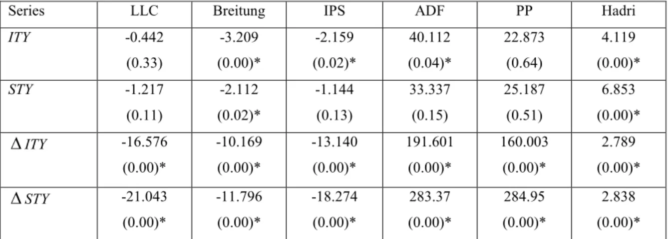
Table 1. Panel Unit Root Tests 1960-2007
Series LLC Breitung IPS ADF PP Hadri
ITY -0.442 (0.33) -3.209 (0.00)* -2.159 (0.02)* 40.112 (0.04)* 22.873 (0.64) 4.119 (0.00)* STY -1.217 (0.11) -2.112 (0.02)* -1.144 (0.13) 33.337 (0.15) 25.187 (0.51) 6.853 (0.00)* ∆ITY -16.576 (0.00)* -10.169 (0.00)* -13.140 (0.00)* 191.601 (0.00)* 160.003 (0.00)* 2.789 (0.00)* ∆STY -21.043 (0.00)* -11.796 (0.00)* -18.274 (0.00)* 283.37 (0.00)* 284.95 (0.00)* 2.838 (0.00)* Notes: Probability values are reported in the parentheses. * denotes the rejection of the null at the 5% level. For a discussion of these tests, see Baltagi (2005) and Pesaran and Breitung (2005).
These tests provide fairly mixed results for ITY. The LLC and PP tests in which the null is that the variable is non-stationary is not rejected at the 5% level. However, in the IPS and ADF tests in which the null is the same accept the null at only the 1% level. In the Hadri test the null is that the variable is stationary and it is rejected at the 5% level. For STY, all the tests show that it is a non-stationary variable at 5% level, except for Breitung at 1% level.
Alternatively, with the exception of the Hadri test, all other tests show that the first
differences of ITY and STY are stationary. Therefore, it is reasonable to conclude that these variables are by and large I(1) in their levels.
The results of the panel cointegration tests are reported in Table 2. In the fixed effects model (FE model, henceforth), the majority of the cointegration tests, 5 out of 7, show that there is cointegration between ITY and STY at the 5% level. Only the panel
ν
and groupσ
test statistics in the FE model are insignificant at the 5% level. The cointegration tests for the random effects model (RE model, henceforth) are the other way i.e., out of these 7 tests only 2 the panel
ν
and group ADF test statistics reject the null of no cointegration. However, it is well known that the two ADF tests have more power against the null and both reject the null of no cointegration in FE model, but in RE model the null is rejected by only one ADF test. Nonetheless we can infer that the ITY and STY are cointegrated and perhaps the estimates based on the FE model are preferable to those with the RE model.Table 2. Panel Cointegration Tests 1960-2007
Test Statistic FE Model RE Model Panel
ν
- statistic 1.375 2.587* Panelσ
- statistic -1.979** -1.389 Panel ρρ- statistic -2.751* -1.248 Panel ADF-statistic -3.438* -1.479 Groupσ
- statistic -0.809 -1.010 Group ρρ- statistic -2.627* -1.147 Group ADF- statistic -4.512* -2.049*Notes: FE Model is fixed effects model and RE Model is random effects model. The test statistics are distributed as N(0,1). * and ** denotes significance, respectively, at 5% and 10% levels.
The results for the panel long run estimators using panel FMOLS are reported in Table 3.4 The estimates of βis around 0.3 and 0.6 in FE and RE models, respectively. This crucial savings retention coefficient is significant at the 5% level. The country specific estimates of
βvary widely and this is not uncommon in the panel data studies.
4
Table 3: Estimates of the Cointegration Coefficients 1960-2007
Dependent Variable: ITY
FE Model RE Model
β 0.304
(6.83)*
0.571 (13.90)*
Notes: FE Model is fixed effects model and RE Model is random effects model. The t-ratiosare in the parentheses and * indicates significance at the 5% level.
3.2. Effects of Bretton Woods and Maastricht Agreements
We shall examine the effects of two important agreements to increase capital mobility viz., the Bretton Woods and Maastricht Agreements.5 For simplicity, we divided our sample into sub-sample periods to capture the effects of Bretton Woods and Maastricht agreements. It is improbable that these two agreements had instantaneous impact on capital mobility from 1972 and 1992 respectively. Hence we assume that a lag of 3 years is reasonable for their effects. Consequently, we select sub-sample periods as 1960-1974 (pre Bretton Woods), 1975-2007 (post Bretton Woods), 1960-1994 (pre Maastricht) and 1995-2007 (post Maastricht). Prior to further discussion, it would be useful to take an overview of what is expected from these sub-sample estimates. Most importantly, we are investigating some evidence on whether the Bretton Woods and Maastricht agreements had any significant effects on the validity of FHP and capital mobility. If they have been effective, it is to be expected that the value of β will decline in the second set of sub-samples to show an increase in the capital mobility.
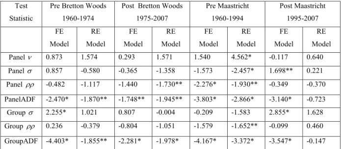
The results of the cointegration tests of the sub-sample periods are reported in Table 4. In the two sets of sub-samples, the null of no cointegration is rejected by the more
powerful ADF test statistics at 10% level, except for RE model in the post-Maastricht period. One or more of the other cointegration tests also confirm cointegration between ITY and STY at 5% level. The only exception is the RE model in the post Maastricht period (1995-2007)
5
The Bretton Woods system of monetary management established the rules for financial relations among the world’s major industrial countries. This agreement started after World War II and ended in 1972. Particularly this agreement established the pegging of currencies and the International Monetary Fund (IMF) in the hope of stabilising the global economic situations. The Maastricht Treaty began from 1992 between the members of the European Community. This agreement created the European Union and led to the creation of the euro.
where all cointegration tests does not reject the null of no cointegration. In light of the above observations, we assert that there is no strong evidence that there is no cointegration in the two sets of sub-sample periods, except for RE model in the post Maastricht period.
Table 4. Panel Cointegration Tests: Subsamples
Test Statistic
Pre Bretton Woods 1960-1974
Post Bretton Woods 1975-2007 Pre Maastricht 1960-1994 Post Maastricht 1995-2007 FE Model RE Model FE Model RE Model FE Model RE Model FE Model RE Model Panel ν 0.873 1.574 0.293 1.571 1.540 4.562* -0.117 0.640 Panel σ 0.857 -0.580 -0.365 -1.358 -1.573 -2.457* 1.698** 0.221 Panel ρρ -0.482 -1.117 -1.440 -1.730** -2.276* -1.930** -0.349 -0.370 PanelADF -2.470* -1.870** -1.748** -1.945** -3.803* -2.866* -3.140* -0.723 Group σ 2.255* 1.021 0.807 -0.004 -0.209 -1.583 2.855* 1.628 Group ρρ 0.236 -0.379 -0.804 -1.051 -1.579 -1.652** -0.099 0.460 GroupADF -4.403* -1.855** -2.281* -1.978* -4.167* -3.372* -3.547* -0.147 Notes: FE Model is fixed effects model and RE Model is random effects model. The t-ratios are in the parentheses and * and ** indicates significance at the 5% and 10% levels, respectively.
Estimates of the cointegrating equations for two sets of sub-samples are reported in Table 5. The pre Bretton Woods period highlights that the estimate of β is 0.467 and 0.742, respectively, in the FE and RE models. In both models the estimate of β has decreased to 0.266 and 0.486, respectively, in the post Bretton Woods period. Similar results are also found between the pre and post Maastricht periods. The estimate of βhas decreased from 0.443 to 0.248 in the FE model and from 0.652 to 0.115 in the RE model. The country specific estimates of βbased on the sub-sample periods are not reported but available from the authors upon request. These results show that for majority of the OECD countries, the estimates of βhas slightly declined due to the Bretton Woods and Maastricht agreements, thus implying that international mobility of capital has marginally increased in these countries.
Table 5 Estimates of the Cointegration Coefficients: Subsamples
Test Statistic
Pre Bretton Woods 1960-1974
Post Bretton Woods 1975-2007 Pre Maastricht 1960-1994 Post Maastricht 1995-2007 FE Model RE Model FE Model RE Model FE Model RE Model FE Model β 0.467 (12.82)* 0.742 (13.73)* 0.266 (6.08)* 0.486 (8.70)* 0.443 (9.34)* 0.652 (17.48)* 0.248 (7.01)* Notes: FE Model is fixed effects model and RE Model is random effects model. The t-ratiosare in the parentheses and * indicates significance at the 5% level.β for RE Model in the post Maastricht period is not reported because all the cointegration tests does not reject the null of no cointegration at 10% level. However, groupσ test statistics does support cointegration at slightly more than 10% level. Therefore, the estimate of
β is 0.115 which is significant at 5% level.
We have also tested for structural breaks using the Westerlund (2006) method. This helps to verify if our choice of the above dates is reasonable. From the late 1960s to the early 1970s the Westerlund method indicated that there have been structural breaks in Denmark (1966), Australia (1972), Great Britain (1970) and Italy (1970). In the other countries the break occurred later in the late 1970s and early 1980s. These countries are Belgium (1981), France (1980), Greece (1983), Ireland (1981), Spain (1983) and the USA (1977). In Germany and Sweden the break seems to have taken place in the late 1980s. There is thus a mixed result that the Bretton Woods agreement had a uniform effect on all the OECD countries to increase capital mobility. This prolonged period for structural adjustments may be due to the differences in the response by these countries to the economic uncertainties of the early 1970s. During this period the Bretton Woods fixed exchange rate system collapsed and was replaced with different managed exchange rate systems. There were high inflation and severe energy crises which in turn encouraged more conservative budgetary and monetary policies as well as some market liberalisation policies. Therefore, an improvement in the international capital mobility seems to have taken place over a longer time span and at different times in different countries.
In contrast the dates for the second break are more uniform and around the late 1980s and the early 1990s. A second structural break occurred in 9 out of the 13 OECD countries and these are Australia (1990), Denmark (1989), France (1996), Great Britain (1990), Ireland (1988), Italy (1992), Spain (1992), Sweden (1995) and the USA (1990). We have also tested for a single structural break. The results showed that there was a break during the late 1980s and early 1990s except in Greece and Ireland. There is no evidence that there was a break in
the early 1970s. It may be recalled that the estimates of βin both the post Bretton Woods and post Maastricht agreements are about 50 percent lower than in the pre-agreement periods. On the basis of the Westerlund tests we may conclude that Maastricht agreement seems to have had a more uniform and widespread effect on improving capital mobility in the major OECD countries. The lower estimate for βin the post Bretton Woods period may be due to the inclusion of the period for the post Maastricht period in this sample.
4. Conclusion
In this paper we have used the time series based panel data methods and data from 13 OECD countries to test the validity of the mother of all puzzles viz., the Feldstein-Horioka puzzle (FHP). FHP has stimulated a large number of empirical works because of its
important implications. It has directly or indirectly implied that international capital mobility was very low even among the advanced capitalist OECD countries. While this finding of Feldstein and Horioka’s seminal contribution might be valid for their sample period of the 1960s and up to the collapse of the Bretton Woods agreement in the early 1970s,
subsequently the turmoil caused by the collapsed fixed exchange rate system and the economic uncertainties of the 1970s led to the implementation of liberalisation policies and reforms, which seems to have improved the international capital mobility. However, the Maastricht agreement of the early 1990s has significantly improved international capital mobility. The saving retention coefficient is halved and less than 0.25 now.
However, our study and conclusions have some limitations. Firstly, the break dates in the Westerlund tests are somewhat sensitive to the selected method of estimation and the number of breaks selected. Secondly, due to data limitations we have included only 13 OECD
countries in our sample. Thirdly, the scope of the software used for the Pedroni estimation method is limited in that it is not possible to use the Wald type 2
χ
tests to test restrictions on the coefficients. Nevertheless, our conclusion that there have been significant structural breaks in the Feldstein-Horioka equation and international capital mobility has improved in the post Bretton Woods and Maastricht periods seems to be robust and valid.Data Appendix
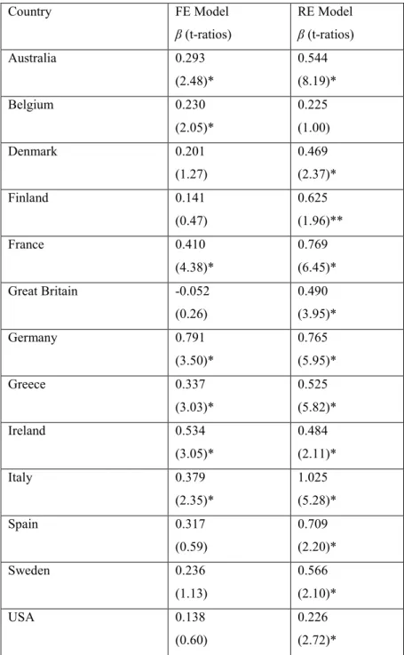
ITY is gross domestic investment as a share of GDP. Data obtained from International Financial Statistics (IFS) 2007.
Table 1A: Pedroni’s Country Specific Estimates 1960-2007 Country FE Model β (t-ratios) RE Model β (t-ratios) Australia 0.293 (2.48)* 0.544 (8.19)* Belgium 0.230 (2.05)* 0.225 (1.00) Denmark 0.201 (1.27) 0.469 (2.37)* Finland 0.141 (0.47) 0.625 (1.96)** France 0.410 (4.38)* 0.769 (6.45)* Great Britain -0.052 (0.26) 0.490 (3.95)* Germany 0.791 (3.50)* 0.765 (5.95)* Greece 0.337 (3.03)* 0.525 (5.82)* Ireland 0.534 (3.05)* 0.484 (2.11)* Italy 0.379 (2.35)* 1.025 (5.28)* Spain 0.317 (0.59) 0.709 (2.20)* Sweden 0.236 (1.13) 0.566 (2.10)* USA 0.138 (0.60) 0.226 (2.72)*
Notes: FE Model is fixed effects model and RE Model is random effects model. The t-ratiosare in the parentheses and * and **indicates significance at the 5% and 10% levels, respectively.
References
Apergis, N. and Tsoumas, C. (2009) ‘A survey on the Feldstein-Horioka puzzle: what has been done and where we stand, Research in Economics, Forthcoming. Also available at SSRN: http://ssrn.com/abstract=993736.
Bahmani-Oskooee, M. and Chakrabarti A. (2005) ‘Openness, size, and the saving-investment relationship,’ Economic Systems, 29, 283-93.
Baltagi, B. H. (2005) Econometric Analysis of Panel Data, Chester, UK: John Wiley, 3rd edition.
Breitung, J. (2000) “The local power of some unit root tests for panel data, in Baltagi, B.(ed.), Advances in Econometrics: Non-stationary panels, panel cointegration, and dynamic panels, JAI Press, Amsterdam, 161-78.
Cadoret, I. (2001) ‘The saving investment relation: a panel data approach,’ Applied Economics Letters, 8, 517–20.
Chakrabarti, A. (2006) ‘The saving-investment relationship revisited: new evidence from multivariate heterogeneous panel co-integration analyses,’ Journal of Comparative Economics, 34, 402-19.
Christopoulos, D. K. (2007) ‘A reassessment of the Feldstein-Horioka hypothesis of perfect capital mobility: evidence from historical data,’ Empirica, 34, 273-80.
Coakley, J., Fuertes, A. M. and Spagnolo, F. (2004) ‘Is the Feldstein-Horioka puzzle history?,’ The Manchester School, 72, 569-90.
Coakley, J., Fuertes, A.-M. and Smith, R. (2001) ‘Small sample properties of panel time- series estimators with i(1) errors,’ Birkbeck College Discussion Paper 3/2001.
Coakley, J., Hasan, F. and Smith, R. (1999) ‘Saving, investment, and capital mobility in LDCs,’ Review of International Economics, 7, 632–40.
Coakley, J. and Kulasi, F. (1997) ‘Cointegration of long span saving and investment,’ Economics Letters, 54, 1-6.
Di Iorio, F. and Fachin, S. (2007) ‘Testing for breaks in cointegrated panels - with an application to the Feldstein-Horioka puzzle,’ Economics - The Access, Open-Assessment E-Journal, 1, 1-30. Also available as Working Paper
http://mpra.ub.unimuenchen.de/3280.
Feldstein, M. and Horioka, C. (1980) ‘Domestic saving and international capital flows,’ Economic Journal, 90, 314-29.
Fouquau, J., Hurlin, C. and Rabaud, I. (2009) ‘The Feldstein-Horioka puzzle: A panel smooth transition regression approach,’ Economic Modelling, 25, 284-99.
Giannone, D. and Lenza, M. (2004) ‘The Feldstein-Horioka fact,’ available at www.ecb.int/pub/pdf/scpwps/ecbwp873.pdf.
Hadri, K. (2000) ‘Testing for stationarity in heterogeneous panel data,’Econometric Journal, 3, 148-61.
Herwartz, H. and Xu, F. (2009) ‘Panel data model comparison for empirical saving-investment relations,’ Applied Economics Letters, Forthcoming.
Im, K.S., M.H. Pesaran and Y. Shin (2003) ‘Testing for unit roots in heterogeneous panels,’ Journal of Econometrics, 115, 53-74.
Jansen, W. J. (1998) ‘Interpreting saving-investment correlations,’ Open Economies Re- View, 9, 205-17.
--- (1996) ‘Estimating saving–investment correlations: evidence for OECD countries based on an error correction model,’ Journal of International Money and Finance, 15, 749-81.
Kim, H., Oh, K.Y.,Jeong, C.W. (2005) ‘Panel cointegration results on international capital mobility in Asian countries,’ Journal of International Money and Finance, 24, 71-82.
Levin, A., C.F. Lin and C. Chu (2002) “Unit root tests in panel data: asymptotic and finite sample properties”, Journal of Econometrics, 108, 1-24.
Murthy, N.R.V. (2007) ‘Feldstein Horioka puzzle in Latin American and Caribbean countries: evidence from likelihood based cointegration tests in heterogenous panels,’ International Research Journal of Finance and Economics, 11, 112-22.
Obstfeld, M. and Rogoff, K. (2000) ‘The six major puzzles in international macroeconomics: Is there a common cause?,’ NBER Macroeconomics Annual, 15, 340-90.
Pelgrin, F. and Schich, S. (2004) ‘National saving-investment dynamics and international capital mobility,’ Working Paper 2004-14, Bank of Canada.
Pesaran, M. H. and Breitung, J., (2005) “Unit roots and cointegration in panels” Discussion Paper Series 1: Economic Studies No 42/2005, Deutsche Bundesbank, Frankfurt, Germany.
Westerlund, J., (2006) “Testing for panel cointegration with multiple structural breaks”, Oxford Bulletin of Economics and Statistics, 68, 101-32.