A Symbol-based Bar Code Decoding Algorithm
Mark A. Iwen∗ Fadil Santosa† Rachel Ward‡
April 25, 2012
Abstract
We investigate the problem of decoding bar codes from a signal measured with a hand-held laser-based scanner. Rather than formulating the inverse problem as one of binary image reconstruction, we instead determine the unknown code from the signal. Our approach has the benefit of incorporating the symbology of the bar code, which reduces the degrees of freedom in the problem. We develop a sparse representation of the UPC bar code and relate it to the measured signal. A greedy algorithm is proposed for for decoding the bar code from the noisy measurements, and we prove that reconstruction through the greedy algorithm is robust both to noise and to unknown parameters in the scanning device. Numerical examples further illustrate the robustness of the method.
1
Introduction
This work concerns an approach for decoding bar code signals. While it is true that bar code scanning is, for the most part, a solved problem, as evidenced by its prevalent use, there is still a need for more reliable decoding algorithms. This need is specialized to situations where the signals are highly corrupted and the scanning takes place in less than ideal situations. It is under these conditions that traditional bar code scanning algorithms often fail.
The problem of bar code decoding may be viewed as a deconvolution of a binary one-dimensional image in which the blurring kernel contains unknown parameters which must be estimated from the signal [5]. Esedoglu [5] was the first to provide a mathematical analysis of the bar code decoding problem in this context. In the article, he established the first uniqueness result of its kind for the problem. He further showed how the blind deconvolution problem can be formulated as a well-posed variational problem. An approximation, based on the Modica-Mortola energy [10], is the basis for the computational approach. The approach has recently been given further analytical treatment in [6].
A recent work [2] deals with the case where the blurring is not very severe. The authors showed rigorously that for the case where the blurring parameters are known, the variational
∗
Mathematics Department, Duke University, Durham, NC 27708, [email protected], research supported in part by ONR N00014-07-1-0625 and NSF DMS DMS-0847388
†
School of Mathematics, University of Minnesota, Minneapolis, MN 55455, [email protected], re-search supported in part by NSF DMS-0807856
‡
Courant Institute of Mathematical Sciences, New York University, New York, NY 10012
formulation of [5] is able to deal with a small amount of blurring and noise. Specifically they showed that the correct bar code can be found by treating the signal as if it arose from a system where no blurring has occurred.
The approach presented in this work departs from the above image-based approaches. We treat the unknown as a finite-dimensional code. A model that relates the code to the measured signal is developed. We show that by exploiting the symbology – the language of the bar code – we can express bar codes as sparse representations in a given dictionary. We develop a recovery algorithm which fits the observed signal to a code from the symbology in a greedy fashion, and we show that the algorithm is fast and robust.
The outline of the paper is as follows. We start by developing a model for the scanning process. In section 3, we study the properties of the UPC (Universal Product Code) bar code and provide a mathematical representation for the code. Section 4 develops the relation between the code and the measured signal. An algorithm for decoding bar code signals is presented in section 5. Section 6 is devoted to the analysis of the algorithm proposed. Results from numerical experiments are presented in Section 7. A final section concludes the work with a discussion.
We were unable to find any previous symbol-based methods for bar code decoding in the open literature. We note that there is an approach for super-resolving scanned images that is symbol based [1]. However, the method in that work is statistical in nature whereas our method is deterministic. Both this work and the super-resolution work are similar in spirit to lossless data compression algorithms known as ‘dictionary coding’ (see, e.g., [11]) which involve matching strings of text to strings contained in an encoding dictionary.
Another related approach utilizes a genetic algorithm for barcode image decoding [3]. In this work the bar code symbology is utilized to help represent populations of candidate barcodes, together with blurring and illumination parameters, which might be responsible for generating the observed image data. Successive generations of candidate solutions are then spawned from those best matching the input data until a stopping criteria is met. In addition to utilizing an entirely different decoding approach, this work also differs from the methods developed herein in that it makes no attempt to either analyze, or utilize, the relationship between the structure of the barcode symbology and the blurring kernel.
2
A scanning model and associated inverse problem
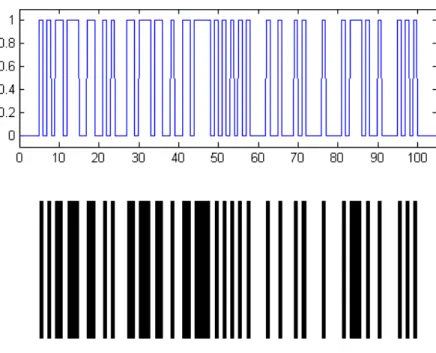
A bar code is scanned by shining a narrow laser beam across the black-and-white bars at constant speed. The amount of light reflected as the beam moves is recorded and can be viewed as a signal in time. Since the bar code consists of black and white segments, the reflected energy is large when the beam is on the white part, and small when the beam is on the black part. The reflected light energy at a given position is proportional to the integral of the product of the beam intensity, which can be modeled as a Gaussian1, and the bar code image intensity (white is high intensity, black is low). The recorded data are samples of the resulting continuous time signal.
Let us write the Gaussian beam intensity as a function of time:
g(t) =α√1
2πσe
−(t2/2σ2). (1)
1This Gaussian model has also been utilized in many previous treatments of the bar code decoding
Figure 1: Samples of the binary bar code function z(t) and the UPC bar code. Note that in UPC bar codes, each bar - black or white - is a multiple of the minimum bar width.
There are two parameters: (i) the variance σ2 and (ii) the constant multiplier α. We will overlook the issue of relating time to the actual position of the laser beam on the bar code, which is measured in distance. We can do this because of the way bar codes are encoded – only relative widths of the bars are important.
Thus let z(t) be the bar code. Since z(t) represents a black and white image, we will normalize it to be a binary function. Then the sampled data are
di=
Z
g(ti−τ)z(τ)dτ+hi, i∈[m], (2)
where theti∈[0, n] are equally spaced discretization points, and thehi represent the noise
associated with scanning. We have used the notation [m] = {1,2, ..., m}. We need to consider the relative size of the laser beam spot to the width of the narrowest bar in the bar code. We set the minimum bar width to be 1 in the artificial time measure.
Next we explain the roles of the parameters in the Gaussian. The variance σ2 models the distance from the scanner to the bar code – longer distance means bigger variance. The width of a Gaussian is defined as the interval over which the Gaussian is greater than half its maximum amplitude, and is given by 2√2 ln 2σ. We will be considering situations where the Gaussian blur width is of the same order as the size as the minimum width of the bars. The multiplierαlumps the conversion from light energy interacting with a binary bar code image to the measurement. Since the distance to the bar code is unknown and the intensity-to-voltage conversion depends on ambient light and properties of the laser/detector, these parameters are assumed to be unknown.
To develop the model further, consider the characteristic function
χ(t) =
1 for 0≤t≤1,
0 else.
Then the bar code function can be written as
z(t) =
n
X
j=1
cjχ(t−(j−1)), (3)
where the coefficientscj are either 0 or 1. The sequence
c1, c2,· · ·, cn,
represents the information stored in the bar code. In the UPC symbology, the digit ‘four’ is represented by the sequence 0100011. This is to be interpreted as a white bar of unit width, followed by a black bar of unit width, followed by a white bar of 3 unit widths, and ended with a black bar of two unit widths. For UPC bar codes, the total number of unit widths,n, is fixed to be 95 for a 12-digit code (further explanations in the subsequent). Remark 2.1 One can think of the sequence{c1, c2,· · · , cn}as an instruction for printing a
bar code. Everyci is a command to lay out a white bar ifci= 0, or a black bar if otherwise.
Substituting the representation (3) back in (2), we get
di = Z g(ti−t) n X j=1 cjχ(t−(j−1)) dt+hi = n X j=1 " Z j (j−1) g(ti−t)dt # cj+hi.
In terms of the matrixG=G(σ) with entries
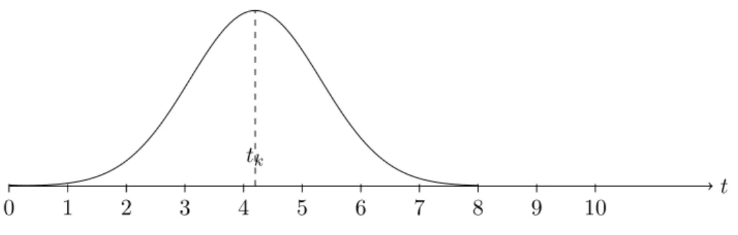
Gkj = 1 √ 2πσ Z j (j−1) e− (tk−t)2 2σ2 dt, k∈[m], j∈[n], (4)
this bar code determination problem reads
d=αG(σ)c+h. (5)
In the sequel, we will assume this discrete version of the bar code problem.
Consider the over-sampling ratio r = m/n. As r increases, meaning that the num-ber of time samples per bar width increases, the matrix G becomes more and more over-determined. More specifically,Gis a nearly block-diagonal matrix with blocks of size≈r×1. This structure will be important below.
While it is tempting to solve (5) directly for c,σ and α, the best approach for doing so is not obvious. The main difficulty stems from the fact that cis a binary vector, while the Gaussian parameters are continuous variables.
tk
0 1 2 3 4 5 6 7 8 9 10 t
Figure 2: The matrix element Gkj is calculated by placing a scaled Gaussian over the bar code grid and integrating over each of the bar code intervals.
3
Incorporating the UPC bar code symbology
We now tailor the bar code reading problem specifically to UPC bar codes. In the UPC-A symbology, a bar code represents a 12-digit number. If we ignore the check-sum requirement, then any 12-digit number is permitted, and the number of unit widths, n, is fixed to 95. Going from left to right, the UPC bar code has 5 parts – the start sequence, the codes for the first 6 digits, the middle sequence, the codes for the next 6 digits, and the end sequence. Thus the bar code has the following structure:
SL1L2L3L4L5L6M R1R2R3R4R5R6E,
whereS,M, and E are the start, middle, and end patterns respectively, andLi and Ri are
patterns corresponding to the digits.
In the sequel, we represent a white bar of unit width by 0 and a black bar by 1 in the bar code representation {ci}.2 The start, middle, and end patterns are
S =E = [101], M = [01010].
The patterns forLi and Ri are taken from the following table:
digit L-pattern R-pattern
0 0001101 1110010 1 0011001 1100110 2 0010011 1101100 3 0111101 1000010 4 0100011 1011100 5 0110001 1001110 6 0101111 1010000 7 0111011 1000100 8 0110111 1001000 9 0001011 1110100 (6)
Note that the right patterns are just the left patterns with the 0’s and 1’s flipped. It follows that the bar code can be represented as a binary vector c ∈ {0,1}95. However, not every
2Note that identifying white bars with 0 and black bars with 1 runs counter to the natural light intensity
binary vector constitutes a bar code – only 2.5×10⁻¹⁷%, or 1012 of the total 295 binary sequences of length 95, are bar codes. Thus the bar code symbology constitutes a very small set; sufficiently small that we can map the set of possible bar codes to a set of structured sparse representations in a certainbar code dictionary.
To form the dictionary, we first write the left-integer and right-integer codes as columns of a 7-by-10 matrix, L= 0 0 0 0 0 0 0 0 0 0 0 0 0 1 1 1 1 1 1 0 0 1 1 1 0 1 0 1 1 0 1 1 0 1 0 0 1 1 0 1 1 0 0 1 0 0 1 0 1 0 0 0 1 0 1 0 1 1 1 1 1 1 1 1 1 1 1 1 1 1 , R= 1 1 1 1 1 1 1 1 1 1 1 1 1 0 0 0 0 0 0 1 1 0 0 0 1 0 1 0 0 1 0 0 1 0 1 1 0 0 1 0 0 1 1 0 1 1 0 1 0 1 1 1 0 1 0 1 0 0 0 0 0 0 0 0 0 0 0 0 0 0 .
The start and end patterns, S and E, are 3-dimensional vectors, while the middle pattern
M is a 5-dimensional vector
S=E = [010]T, M = [01010]T The bar code dictionary is the 95-by-123 block diagonal matrix
D= S 0 . . . 0 0 L ... .. . L L L L L M R R R R R ... .. . R 0 0 . . . 0 E .
Bar codes ccan be expanded with respect to D as
where
1. The 1st, 62nd and the 123rd entries ofx, corresponding to theS,M, andE patterns, are 1.
2. Among the 2nd through 11th entries ofx, exactly one entry – the entry corresponding to the first digit inc=Dx– is nonzero. The same is true for 12th through 22nd entries, etc, until the 61st entry. This pattern starts again from the 63rd entry through the 122th entry. In all,x has exactly 15 nonzero entries.
That is, x must take the form
xT = [1, v1T,· · · , v6T,1, v7T,· · ·, vT12,1], (8) wherevj, forj= 1,· · ·,12, are vectors in{0,1}10 having only one nonzero element.
Incorporating this new representation, the bar code determination problem (5) becomes
d=αG(σ)Dx+h, (9)
where the matrices G(σ) ∈ Rm×95 and D ∈ {0,1}95×123 are as defined in (4) and (7)
respectively, andh∈Rm is additive noise. Note that G will generally have more rows than
columns, whileD has fewer rows than columns. Given the datad∈Rm, our objective is to
return a valid bar codex∈ {0,1}123 as reliably and quickly as possible.
4
Properties of the forward map
Incorporating the bar code dictionary into the inverse problem (9), we see that the map between the bar code and observed data is represented by the matrix P = αG(σ)D ∈
Rm×123. We will refer toP =P(α, σ) as theforward map.
4.1 Near block-diagonality
Based on the block-diagonal structure of the bar code dictionary D, it makes sense to partitionP as P = h P(1) P(2) . . . P(15) i . (10)
The 1st, 8th, and 15th sub-matrices are special as they correspond to the start, middle, and end sequence of the bar code. Recalling the structure ofxwherec=Dx, these sub-matrices must be column vectors of lengthm which we write as
P(1)=p(1)1 , P(8) =p(8)1 , and P(15)=p(15)1 .
The remaining sub-matrices are m-by-10 nonnegative real matrices and we write each of them as
P(j)=hp(1j) p2(j) . . . p(10j)i, j 6= 1,8,15, (11) where eachp(kj),k= 1,2, ...,10, is a column vector of lengthm. For reasonable levels of blur
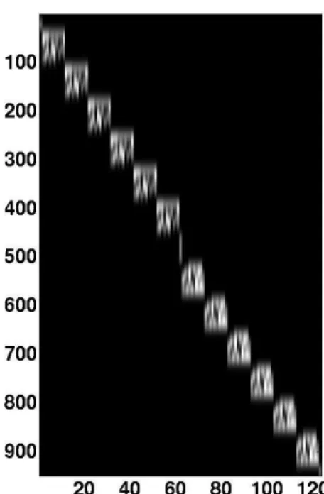
σ in the Gaussian kernel, the forward map P inherits an almost block-diagonal structure from D; we illustrate this in Figure 3. In the limit as σ →0, the forward map P becomes exactly block-diagonal.
Figure 3: A representative bar code forward mapP =αG(σ)Dcorresponding to parameters
r= 10, α= 1, andσ = 1.5.
Recall the over-sampling rate r=m/n which indicates the number of time samples per minimal bar code width. Let us partition the rows of P into 15 blocks, each block with index set Ij of size |Ij|, to indicate the block-diagonal structure. We know that if P(1)
and P(15)correspond to samples of the 3-bar sequence black-white-black, |I1|=|I15|= 3r.
The sub-matrix P(8) corresponds to the signal from 5 bars so |I8|= 5r. Each remaining
sub-matrix corresponds to a signal from a digit of length 7 bars, therefore |Ij| = 7r for
j6= 1,8,15.
We can now give a quantitative measure describing how ‘block-diagonal’ the forward map is. To this end, letεbe the infimum of all >0 which satisfy both
p(kj) [m]\Ij 1 < , for all j∈[15], k ∈[10], (12) and 15 X j0=j+1 p(kj0) j0 Ij 1
< , for all j∈[15], and choices of kj+1, . . . , k15∈[10]. (13)
These inequalities have an intuitive interpretation. The magnitude of ε indicates to what extent the energy of each column of P is localized within its proper block.
As suggested in Figure 4, we find empirically that the value of εin the forward map P
depends on the parametersr andσ according toε= (2/5)σr. By linearity of the map with respect toα, this implies that more generallyε= (2/5)ασr.
0 0.5 1 1.5 0 2 4 6 m ¡ 0 0.5 1 1.5 0 4 8 12 m ¡
Figure 4: For oversampling ratios r = 10 (left) and r = 20 (right), we plot as a function of σ the observed minimal value for εwhich satisfies (12), (13). The thin line in each plot represents (2/5)σr.
4.2 Column incoherence
We now highlight another key property of the forward map P. The left-integer and right-integer codes for the UPC bar code, as enumerated in Table (6), were designed to be well-separated: the `1-distance between any two distinct codes is greater than or equal to
2. Consequently, ifDk are the columns of the bar code dictionaryD, then mink16=k2kDk1−
Dk2k1 = 2. This implies for the forward map P =αG(σ)Dthat when there is no blur, i.e. σ= 0, then µ:= min k16=k2 p (j) k1 −p (j) k2 1= mink16=k2 p(k1j) Ij −p(k2j) Ij 1 = 2αr, (14)
where r is the over-sampling ratio. As the blur in the Gaussian increases from zero, µ=
µ(σ, α, r) should decrease smoothly. In Figure 5 we plot the empirical value of µversus σ
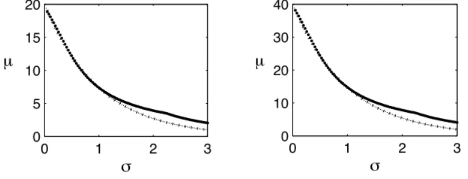
for different values of r. We observe that µ decreases according toµ≈2αre−σ, at least in the range σ≤1. 0 1 2 3 0 5 10 15 20 m µ 0 1 2 3 0 10 20 30 40 m !
Figure 5: For oversampling ratios r = 10 (left) and r = 20 (right), we plot the minimal column separationµ= mink16=k2
p (j) k1 −p (j) k2
1for the forward mapP =G(σ)Das a function of the blur parameter σ. The plots suggest thatµ≈2αre−σ forσ≤1.
5
A simple decoding procedure for UPC bar codes
We know from the bar code determination problem (9) that without additive noise, the observed datadis the sum of 15 columns fromP, one column from each blockP(j). Based on this observation, we will employ a reconstruction algorithm which, once initialized, selects the column from the successive block to minimize the norm of the data remaining after the column is subtracted. This greedy algorithm is described in pseudo-code as follows.
Algorithm 1: Recover Bar Code
initialize:
for `= 1,62,123, x`= 1
else x`= 0
δ ←d
for j = 2 : 7, 9 : 14
kmin= arg mink
δ−p (j) k 1 if j≤7, `←1 + 10(j−2) +kmin else `←62 + 10(j−9) +kmin x`←1 r ←δ−p(kminj) end
6
Analysis of the algorithm
Algorithm 1 recovers the bar code one digit at a time by iteratively scanning through the observed data. The runtime complexity of the method is dominated by the 12 calculations ofkmin performed by the algorithm’s single loop over the course of its execution. Each one
of these calculations ofkminconsists of 10 computations of the`1-norm of a vector of length m.3 Thus, the runtime complexity of the algorithm is O(m).
6.1 Recovery of the unknown bar code
Recall that the 12 unknown digits in the unknown bar codecare represented by the sparse vector x in c = Dx. We already know that x1 = x62 = x123 = 1 as these elements
corresponds to the mandatory start, middle, and end sequences. Assuming for the moment that the forward map P is known, i.e., that both σ and α are known, we now prove that the greedy algorithm will reconstruct the correct bar code from noisy data d=Px+h as long asP is sufficiently block-diagonal and if its columns are sufficiently incoherent. In the next section we will extend the analysis to the case where σ and α are unknown.
3
In practice, whenσis not too large, a smaller ‘windowed’ vector of length less thanmcan be used to approximate δ−p (j) k
1 for eachk, j. This can reduce the constant of proportionality associated with the
Theorem 1 Suppose I1, . . . , I15 ⊂[m] and ε∈ R satisfy the conditions (12)-(13). Then,
Algorithm 1 will correctly recover a bar code signalx given noisy data d=Px+h provided
that p(k1j) Ij − p(k2j) Ij 1 >2 h|Ij 1+ 2ε (15) for all j∈[15] andk1, k2∈[10] with k1 6=k2.
Proof: Suppose that d=Px+h= 15 X j=1 p(kj) j +h.
Furthermore, denoting kj =kmin in the for-loop in Algorithm 1, suppose thatk2, . . . , kj0−1 have already been correctly recovered. Then the residual data, δ, at this stage of the algorithm will be δ=p(kj0) j0 +δj 0 +h, whereδj0 is defined to be δj0 = 15 X j=j0+1 p(kj) j.
We will now show that thej0th execution of the for-loop will correctly recoverp(kj0)
j0 , thereby
establishing the desired result by induction.
Suppose that the j0th execution of the for-loop incorrectly recovers kerr 6= kj0. This happens if δ−p (j0) kerr 1 ≤ δ−p (j0) kj0 1.
In other words, we have that δ−p (j0) kerr 1 = δ Ij0 − p(kerrj0) Ij0 1 + δ Ic j0 − p(kerrj0) Ijc0 1 ≥ p(kj0) j0 I j0 −p(kerrj0) I j0 1 − δj0 Ij0 1 − h Ij0 1 + δj0Ic j0 +hIc j0 1 − p(kj00) j Ijc0 1 − p(kerrj0) Ic j0 1 ≥ p(kj0) j0 Ij0 −p(kerrj0) Ij0 1 + δj0 Ic j0 +h Ic j0 1 − h Ij0 1 −3ε
from conditions (12) and (13). To finish, we simply simultaneously add and subtract
kδj0|I
thatkerr6=kj0: δ−p (j0) kerr 1≥ p(j 0) kj0 Ij0 − p(j 0) kerr Ij0 1 −2 h Ij0 1 −4ε +δj0+h 1 = p(j 0) kj0 Ij0 − p(j 0) kerr Ij0 1 −2 h Ij0 1 −4ε + δ−p (j0) kj0 1 > δ−p (j0) kj0 1. (16)
Remark 6.1 Using the empirical relationships ε= (2/5)αrσand µ= 2αre−σ,the condi-tion (15) is bounded by min j,k16=k2 p(k1j) Ij −p(k2j) Ij 1 ≥ min j,k16=k2 p (j) k1 −p (j) k2 1−2ε= 2αre −σ−(4/5)αrσ,
and we arrive at the following upper bound on the tolerable level of noise for successful recovery: max j∈[12] h|Ij 1≤αr(e −σ−(6/5)σ). (17)
In practice the width 2p2 ln(2)σof the Gaussian blur is on the order of the minimum width of the bar code, which we have normalized to be 1. This translates to a standard deviation of σ≈.425, and in this case the noise tolerance reduces to
max j∈[12] h|Ij 1≤.144αr. (18)
Remark 6.2 In practice it may be beneficial to apply Algorithm 1 several times, each time changing the order in which the digits are decoded. For example, if the distribution of the noise is known in advance, it would be beneficial to to initialize the algorithm in regions of the bar code with less noise.
6.2 Stability of Algorithm 1 with respect to parameter estimation
Insensitivity to unknown α
In the previous section it was assumed that the Gaussian convolution matrix αG(σ) was known. In fact, this is generally not the case. In practice both σ and α must be estimated since these parameters depend on the distance from the scanner to the bar code, the reflec-tivity of the scanned surface, the ambient light, etc. Ultimately this means that Algorithm 1 will be decoding bar codes using only an approximation to αG(σ), and not the true ma-trix itself. Given an approximationσb to the blur σ, we consider the matrix G(bσ), and we describe a procedure for approximating the scaling factor α from this approximation.
Our inverse problem reads
d = αG(σ)Dx+h = αG(σb)Dx+ h+α G(σ)− G(bσ) Dx = αG(σb)Dx+h 0 ; (19)
that is, we have incorporated the error incurred byσbinto the additive noise vectorh0. Note that the middle portion of the observed data dmid=d|I8 of length 5r represents a blurry
image of the known middle pattern M = [01010]. Let P = G(bσ)D be the forward map generated byσb and α= 1, and consider the sub-matrix
pmid= P(8)
I8
which is a vector of length 5r. Ifσb=σthen we can estimateαvia the least squares estimate b
α= arg min
α kαpmid−dmidk2=p T
middmid/k pmidk22. (20)
Ifσb≈σ and the magnitude of the scanning noise,h, is small, we expectαb≈α.
4
Dividing both sides of the equation (19) by αb, the inverse problem becomes
d b α = α b αG(σb)Dx+ 1 b αh 0. (21)
Suppose that 1−γ ≤ α/αb ≤ 1 +γ for some 0 < γ < 1. Then fixing the data to be b
d=d/αb and fixing forward map to beP =G(bσ)D, the recovery conditions (12), (13), and (15) become respectively 1. p(kj) [m]\Ij 1
< 1+εγ for all j∈[15] andk∈[10].
2. P15 j0=j+1p(j 0) kj0 Ij 1
< 1+εγ for allj ∈[14] and validkj0 ∈[10].
3. p(k1j) Ij −p(k2j) Ij 1 >2α1 h|Ij 1+ G(σ)− G(σb) Dx Ij 1+ 2ε 1−γ
Consequently, if σ ≈σb and 1/α ≈ αb, the conditions for correct bar code reconstruction do not change much.
Insensitivity to unknown σ
We have seen that one way to estimate the scaling α is to guess a value forσ and perform a least-squares fit of the observed data. In doing so, we found that the sensitivity of the recovery process with respect toσ is proportional to the quantity
(G(σ)− G(bσ))Dx|Ij 1 (22)
in the third condition immediately above. Note that all the entries of the matrix (G(σ)− G(bσ)) will be small wheneverbσ≈σ. Thus, Algorithm 1 should be able to tolerate small parameter estimation errors as long as the “almost” block diagonal matrix formed usingσb exhibits a sizable difference between any two of its digit columns which might (approximately) appear in any position of a given UPC bar code.
4Here we have assumed that the noise level is low. In noisier settings it should be possible to develop
To get a sense of the size of this term, let us further investigate the expressions involved. Recall that using the dictionary matrix D, a bar code sequence of 0’s and 1’s is given by
c=Dx. When put together with the bar code function representation (3), we see that [G(σ)Dx]i= Z gσ(ti−t)z(t)dt, where gσ(t) = 1 √ 2πσe −( t2 2σ2). Therefore, we have [G(σ)Dx]i = n X j=1 cj Z j j−1 gσ(ti−t)dt. (23)
Now, using the definition for the cumulative distribution function for normal distributions Φ(x) = √1 2π Z x −∞ e−t2/2dt, we see that Z j j−1 gσ(ti−t)dt= Φ ti−j+ 1 σ −Φ ti−j σ .
and we can now rewrite (23) as [G(σ)Dx]i = n X j=1 cj Φ ti−j+ 1 σ −Φ ti−j σ .
We now isolate the term we wish to analyze: [(G(σ)− G(bσ))Dx]i = n X j=1 cj Φ ti−j+ 1 σ −Φ ti−j+ 1 b σ −Φ ti−j σ + Φ ti−j b σ .
We are interested in the error
|[(G(σ)− G(σb))Dx]i| ≤ n X j=1 cj Φ ti−j+ 1 σ −Φ ti−j+ 1 b σ −Φ ti−j σ + Φ ti−j b σ ≤ n X j=1 Φ ti−j+ 1 σ −Φ ti−j+ 1 b σ + Φ ti−j σ −Φ ti−j b σ , ≤ 2 n X j=0 Φ ti−j σ −Φ ti−j b σ .
Suppose thatξ = (ξk) is the vector of values|ti−j|for fixedi, runningj, sorted in order
of increasing magnitude. Note that ξ1 and ξ2 are less than or equal to 1, andξ3 ≤ξ1+ 1, ξ4 ≤ξ2+ 1, and so on. We can center the previous bound around ξ1 and ξ2, giving
|[(G(σ)− G(bσ))Dx]i| ≤ n X j=0 Φ ξ1+j σ −Φ ξ1+j b σ + Φ ξ2+j σ −Φ ξ2+j b σ .(24)
Next we simply majorize the expression f(x) = Φx σ −Φx b σ .
To do so, we take the derivative and find the critical points, which turn out to be
x∗ =±√2σσb r logσ−logσb σ2− b σ2 .
Therefore, each term in the summand (24) can be bounded by Φ ξ+j σ −Φ ξ+j b σ ≤ Φ √ 2bσ r logσ−logbσ σ2− b σ2 ! −Φ √ 2σ r logσ−logbσ σ2− b σ2 ! := 41(σ,bσ). (25)
On the other hand, the terms in the sum decrease exponentially as j increases. To see this, recall the simple bound
1−Φ(x) = √1 2π Z ∞ x e−t2/2dt ≤ √1 2π Z ∞ x t xe −t2/2 dt = e −x2/2 x√2π.
Writing σmax = max{(σ,bσ)}, and noting that Φ(x) is a positive, increasing function, we have for ξ∈[0,1) Φ ξ+j σ −Φ ξ+j b σ ≤ 1−Φ ξ+j σmax ≤ σmax (ξ+j)√2πe −(ξ+j)2/(2σ2 max) ≤ σmax (ξ+j)√2πe −(ξ+j)/(2σmax2 ) ifj≥1 = σmax (ξ+j)√2π e−(2σ2max)−1 ξ+j ≤ σmax j√2π e−(2σmax2 )−1 j := ∆2(σmax, j). (26)
Combining the bounds (25) and (26), Φ ξ+j σ −Φ ξ+j b σ ≤min (41(σ,σb),42(σmax, j) .
Suppose thatj1 is the smallest integer in absolute value such that42(σmax, j1)≤ 41(σ,σb). Then from this term on, the summands in (24) can be bounded by a geometric series:
n X j≥j1 Φ ξ+j σ −Φ ξ+j b σ ≤ 2σmax j1 √ 2π X j≥j1 aj, a=e−(2σmax2 )−1 ≤ 2σmax j1 √ 2π ·a j1(1−a)−1.
We then arrive at the bound |[(G(σ)− G(σb))Dx]i| ≤ 2·j141(σ,σb) + 4σmax·aj1(1−a)−1 j1 √ 2π =: B(σ,σb). (27)
The term (22) can then be bounded according to (G(σ)− G(σb))Dx|Ij 1 ≤ |Ij|B(σ,σb)≤7rB(σ,σb), (28) wherer =m/n is the over-sampling rate.
Recall that in practice the width 2p2 ln(2)σ of the Gaussian kernel is on the order of 1, the minimum width of the bar code, givingσ ≈.425. Below, we compute the error bound
B(σ,bσ) for σ=.425 and several values ofbσ. b
σ 0.2 0.4 .5 0.6 .8
B(.425,bσ) .3453 .0651 .1608 .3071 .589
While the bound (28) is very rough, note that the tabulated error bounds incurred by inaccurateσ are at least roughly the same order of magnitude as the empirical noise level tolerance for the greedy algorithm, as discussed in Remark 6.1.
7
Numerical Evaluation
In this section we illustrate with numerical examples the robustness of the greedy algorithm to signal noise and imprecision in theαandσ parameter estimates. We assume that neither
α nor σ is known a priori, but that we have an estimate bσ for σ. We then compute an estimate αb fromσb by solving the least-squares problem (20).
The phase diagrams in Figure 6 demonstrate the insensitivity of the greedy algorithm to relatively large amounts of noise. These diagrams were constructed by executing a greedy recovery approach along the lines of Algorithm 1 on many trial input signals of the form
d=αG(σ)Dx+h, wherehis mean zero Gaussian noise. More specifically, each trial signal,d, was formed as follows: First, a 12 digit number was generated uniformly at random, and its associated blurred bar code,αG(σ)Dx, was formed using the oversampling ratior=m/n= 10. Second, a noise vectorn, with independent and identically distributednj ∼ N(0,1), was
generated and then rescaled to form the additive noise vectorh=νkαG(σ)Dxk2(n/knk2).
Hence, the parameterν = khk2
kαG(σ)Dxk2 represents the noise-to-signal ratio of each trial input
signald.
We note that in laser-based scanners, there are two major sources of noise. First is electronic noise [8], which is often modeled by 1/f noise [4]. Second, the roughness of the paper also causes speckle noise [9]. In our numerical experiments, however, we simply used numerically generated Gaussian noise, which we believe is sufficient for the purpose of this work.
To create both phase diagrams in Figure 6 the greedy recovery algorithm was run on 100 independently generated trial input signals for each of at least 100 equally spaced (σ, νb ) grid points (a 10×10 mesh was used for Figure 6(a), and a 20×20 mesh for Figure 6(b)).
(a) True parameter values: σ=.45,α= 1. (b) True parameter values: σ=.75,α= 1
Figure 6: Recovery Probabilities when α = 1 for two true σ settings. The shade in each phase diagram corresponds to the probability that the greedy algorithm will correctly re-cover a randomly selected bar code, as a function of the relative noise-to-signal level,
ν = khk2
kαG(σ)Dxk2, and the σ estimate, bσ. Black represents correct bar code recovery with probability 1, while pure white represents recovery with probability 0. Each data point’s shade (i.e., probability estimate) is based on 100 random trials.
The number of times the greedy algorithm successfully recovered the original UPC bar code determined the color of each region in the (bσ, ν)-plane. The black regions in the phase diagrams indicate regions of parameter values where all 100 of the 100 randomly generated bar codes were correctly reconstructed. The pure white parameter regions indicate where the greedy recovery algorithm failed to correctly reconstruct any of the 100 randomly generated bar codes.
Looking at Figure 6 we can see that the greedy algorithm appears to be highly robust to additive noise. For example, when the σ estimate is accurate (i.e., when σb ≈ σ) we can see that the algorithm can tolerate additive noise with Euclidean norm as high as 0.25kαG(σ)Dxk2. Furthermore, asbσbecomes less accurate the greedy algorithm’s accuracy appears to degrade smoothly.
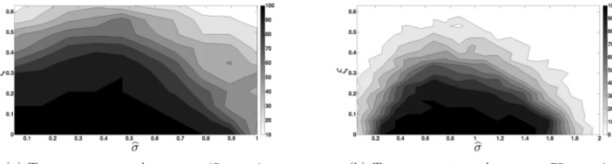
The phase diagrams in Figures 7 and 8 more clearly illustrate how the reconstruction capabilities of the greedy algorithm depend on σ, α, the estimate of σ, and on the noise level. We again consider Gaussian additive noise on the signal, i.e. we consider the inverse problem d = αG(σ)Dx+h, with independent and identically distributed hj ∼ N(0, ξ2),
for several noise standard deviation levels ξ∈[0, .63]. Note thatE h|Ij
1
= 7rξp2/π.5 Thus, the numerical results are consistent with the bounds in Remark 6.1. Each phase diagram corresponds to different underlying parameter values (σ, α), but in all diagrams we fix the oversampling ratio at r =m/n = 10. As before, the black regions in the phase diagrams indicate parameter values (bσ, ξ) for which 100 out of 100 randomly generated bar codes were reconstructed, and white regions indicate parameter values for which 0 out of 100 randomly generated bar codes were reconstructed.
Comparing Figures 7(a) and 8(a) with Figures 7(b) and 8(b), respectively, we can see that the greedy algorithm’s performance appears to degrade with increasing σ. Note that this is consistent with our analysis of the algorithm in Section 6. Increasing σ makes the forward mapP =αG(σ)D less block diagonal, thereby increasing the effective value ofεin conditions (12) and (13). Hence, condition (17) will be less likely satisfied as σ increases.
5This follows from the fact that the first raw absolute moment of eachh
j,E(|hj|), isξ p
(a) True parameter values: σ=.45,α= 1. (b) True parameter values: σ=.75,α= 1
Figure 7: Recovery probabilities when α = 1 for two true σ settings. The shade in each phase diagram corresponds to the probability that the greedy algorithm correctly recovers a randomly selected bar code, as a function of the additive noise standard deviation, ξ, and theσ estimate,σb. Black represents correct bar code recovery with probability 1, while pure white represents recovery with probability 0. Each data point’s shade (i.e., probability estimate) is based on 100 random trials.
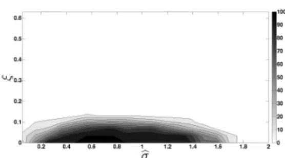
Comparing Figures 7 and 8 reveals the effect of α on the likelihood that the greedy algorithm correctly decodes a bar code. Asαdecreases from 1 to.25 we see a corresponding deterioration of the greedy algorithm’s ability to handle additive noise of a given fixed standard deviation. This is entirely expected sinceα controls the magnitude of the blurred signal αG(σ)Dx. Hence, decreasing α effectively decreases the signal-to-noise ratio of the measured input data d.
Finally, all four of the phase diagrams in Figures 7 and 8 demonstrate how the greedy algorithm’s probability of successfully recovering a randomly selected bar code varies as a function of the noise standard deviation, ξ, and σ estimation error, |σb−σ|. As both the noise level and σ estimation error increase, the performance of the greedy algorithm smoothly degrades. Most importantly, we can see that the greedy algorithm is relatively robust to inaccurate σ estimates at low noise levels. When ξ ≈ 0 the greedy algorithm appears to suffer only a moderate decline in reconstruction rate even when|bσ−σ| ≈σ.
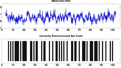
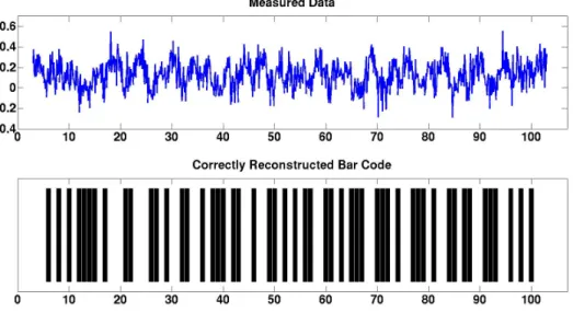
Figure 9 gives examples of two bar codes which the greedy algorithm correctly recovers whenα= 1, one for each value ofσpresented in Figure 7. In each of these examples the noise standard deviation,ξ, and estimatedσvalue,σb, were chosen so that they correspond to dark regions of the example’s associated phase diagram in Figure 7. Hence, these two examples represent noisy recovery problems for which the greedy algorithm correctly decodes the underlying UPC bar code with relatively high probability.6 Similarly, Figure 10 gives two examples of two bar codes which the greedy algorithm correctly recovered when α = 0.25. Each of these examples has parameters that correspond to a dark region in one of the Figure 8 phase diagrams.
6
Theξandbσvalues were chosen to correspond to dark regions in a Figure 7 phase diagram, not necessarily
(a) True parameter values: σ=.45,α=.25. (b) True parameter values: σ=.75,α=.25
Figure 8: Recovery Probabilities when α = .25 for two true σ settings. The shade in each phase diagram corresponds to the probability that the greedy algorithm will correctly recover a randomly selected bar code, as a function of the additive noise standard deviation,
ξ, and the σ estimate, σb. Black represents correct bar code recovery with probability 1, while pure white represents recovery with probability 0. Each data point’s shade (i.e., probability estimate) is based on 100 random trials.
8
Discussion
In this work, we present a greedy algorithm for the recovery of bar codes from signals measured with a laser-based scanner. So far we have shown that the method is robust to both additive Gaussian noise and parameter estimation errors. There are several issues that we have not addressed that deserve further investigation. First, we assumed that the start of the signal is well determined. By the start of the signal, we mean the time on the recorded signal that corresponds to when the laser first strikes a black bar. This assumption may be overly optimistic if there is a lot of noise in the signal. We believe, however, that the algorithm is not overly sensitive to uncertainties in the start time. Of course this property needs to be verified before we can implement the method in practice.
Second, while our investigation shows that the algorithm is not sensitive to the parameter
σ in the model, we did not address the best means for obtaining reasonable approximations of σ. In applications where the scanner distance from the bar code may vary (e.g., with handheld scanners) other techniques for determiningbσ will be required. Given the robust-ness of the algorithm to parameter estimation errors it may be sufficient to simply fixσbto be the expected optimal σ parameter value in such situations. In situations where more accuracy is required, the hardware might be called on to provide an estimate of the scanner distance from the bar code it is scanning, which could then be used to help produce a rea-sonablebσvalue. In any case, we leave more careful consideration of methods for estimating
σ to future work.
Finally we made an assumption that the intensity distribution is well modeled by a Gaussian. This may not be sufficiently accurate for some distances between the scanner and the bar code. Since intensity profile as a function of distance can be measured, one can conceivably refine the Gaussian model to capture the true behavior of the intensities.
References
[1] M. Bern and D. Goldberg, Scanner-model-based document image improvement, Pro-ceedings. 2000 International Conference on Image Processing, IEEE 2000, 582-585. [2] R. Choksi and Y. van Gennip, Deblurring of one-dimensional bar codes via total
vari-ation energy minimisvari-ation,SIAM J. Imaging Sciences,3-4(2010), 735-764.
[3] L. Dumas, M. El Rhabi and G. Rochefort, An evolutionary approach for blind deconvo-lution of barcode images with nonuniform illumination,IEEE Congress on Evolutionary Computation, 2011, 2423-2428.
[4] P. Dutta and P. M. Horn, Low-frequency fluctuations in solids: 1/f noise, Rev. Mod. Phys.,53-3 (1981), 497-516.
[5] S. Esedoglu, Blind deconvolution of bar code signals, Inverse Problems, 20 (2004), 121-135.
[6] S. Esedoglu and F. Santosa, Analysis of a phase-field approach to bar-code deconvolu-tion, preprint 2011.
[7] J. Kim and H. Lee, Joint nonuniform illumination estimation and deblurring for bar code signals,Optic Express,15-22(2007), 14817-14837.
[8] S. Kogan, Electronic Noise and Fluctuations in Solids, Cambridge University Press, 1996.
[9] E. Marom, S. Kresic-Juric and L. Bergstein, Analysis of speckle noise in bar-code scanning systems,J. Opt. Soc. Am.,18(2001), 888-901.
[10] L. Modica and S. Mortola, Un esempio di Γ–convergenza, Boll. Un. Mat. Ital.,5-14 (1977), 285-299.
[11] D. Salomon, Data Compression: The Complete Reference, Springer-Verlag New York Inc, 2004.
(a) True parameter values: σ=.45,α= 1. Estimatedbσ=.3 and Noise Standard Deviationξ=.3. Solving the least-squares problem (20) yields anαestimate ofαb=.9445 fromσb. The relative noise-to-signal level, ν= khk2
kαG(σ)Dxk2, is 0.4817.
(b) True parameter values: σ=.75,α= 1. Estimatedσb= 1 and Noise Standard Deviationξ=.2. Solving the least-squares problem (20) yields anαestimate ofαb= 1.1409 fromσb. The relative noise-to-signal level,
ν= khk2
kαG(σ)Dxk2, is 0.3362.
Figure 9: Two example recovery problems corresponding to dark regions in each of the phase diagrams of Figure 7. These recovery problems are examples of problems with α = 1 for which the greedy algorithm correctly decodes a randomly selected UPC bar code approximately 80% of the time.
(a) True parameter values: σ=.45,α=.25. Estimatedσb=.5 and Noise Standard Deviationξ=.1. Solving the least-squares problem (20) yields anαestimate ofαb= 0.2050 fromσb. The relative noise-to-signal level,
ν= khk2
kαG(σ)Dxk2, is 0.7001.
(b) True parameter values: σ =.75, α =.25. Estimated σb= .8 and Noise Standard Deviation ξ = .06. Solving the least-squares problem (20) yields an α estimate ofαb = 0.3057 from σb. The relative
noise-to-signal level,ν= khk2
kαG(σ)Dxk2, is 0.4316.
Figure 10: Two example recovery problems corresponding to dark regions in each of the phase diagrams of Figure 8. These recovery problems are examples of problems with α =
.25 for which the greedy algorithm correctly decodes a randomly-selected UPC bar code approximately 60% of the time.