Noncritical String Theory

(1)

Noncritical String Theory

Sander Walg

Master’s thesis

Supervisor: Prof. Dr. Jan de Boer

University of Amsterdam Institute for Theoretical Physics

Valckenierstraat 65 1018 XE Amsterdam

The Netherlands August 26, 2008

(2)

(3)

Abstract

In strings theory, a critical dimension, Dc is required to yield consistent

theories. For bosonic strings Dc = 26 and for superstringsDc = 10. These

numbers arise naturally from the theory itself. Less familiar are noncrit-ical string theories, theories with D 6= Dc. These theories emerge when

background fields are included to the theory, in particular linear dilaton backgrounds. We will study quintessence-driven cosmologies and show an analogy between them and string theories in a timelike linear dilaton theory. We will also present a set of exact solutions for the linear dilaton-tachyon profile system that gives rise to a bubble of nothing. Generalizing this set-ting induces a dimension-changing bubble, which can also be solved exactly at one-loop order. Eventually, we will consider transitions from one theory to another. In this way, noncritical string theories can be connected to the familiar web of critical string theories. Surprisingly, transitions from su-perstring theories can yield pure bosonic theories. Our main focus will be bosonic strings.

(4)

(5)

Preface

Foreword

When I started writing my thesis, I was immediately confronted with a tremendous abundancy of background material on string theory. Even though string theory is relatively new, already a lot of books and an enor-mous amount of articles have been written on the subject, and the level of difficulty varies greatly. Some books were very advanced, others were much more comprehensible but somewhat limited in detail. I found it was a challenging task to restrict my focus only on those subjects relevant to the scope of this thesis, because it is very easy to get lost in all the fascinating features and idea’s that are indissoluble connected to string theory.

At first I had some doubt whether I should go into a lot of detail with calculations or not. But gradually, I found that I gained most satisfaction out of explaining most of the intermediate steps needed to complete a cal-culation, whenever I thought they contributed to the clarity of the subject. Whenever a calculation would become to detailed or advanced, I decided to give a reference to the book or article the problem can be found in.

I wrote this thesis on the level of graduate students, with preliminary knowledge on quantum field theory, general relativity and string theory. Only chapter 3 involves some knowledge on algebra and representations. It will not be used later on. With this in mind, I still tried to make the thesis as self-contained as possible, reviewing some general facts where needed.

Just as many people before me, I too found out that writing a thesis is by far the most challenging and difficult task of completing my studies as a physics student. Nevertheless, I’ve experienced this as a very educative and enjoyable time, and during this period I found out that my interest in doing theoretical research has grown considerably.

Acknowledgments

First of all, I would like to thank my supervisor Jan de Boer, who has always been an inspiration to me and could explain difficult subject in a very clear way. I always enjoyed his lectures a lot and his interpretations truly made

(6)

complicated subjects completely comprehensible.

Secondly, I would like to thank my student friends who were always open to questions and discussions and who helped me with some difficulties regarding LA_TEX.

I also like to thank my other friends, who never lost faith in me and always helped me regain new energy. They always showed a lot of interest in my studies and my thesis, and in turn I enjoyed explaining them the exotic features of particle physics, cosmology, black holes and string theory. I would like to thank my girlfriend Sabine Wirz, who often found me completely worn out after a long day at the university and who has always been there for me. She supported me a great deal and absolutely helped me through this period.

And finally I would like to thank my family, who I could rely on all my years at University. In particular I would like to thank my father, Hugo Walg, who somehow always managed to get the best out of me and supported me with his technical backup. And last, I would like to thank my mother, Doroth´ee van Wijhe, who was always able to motivate me, and who made it possible for me to graduate this year. I don’t think I could have succeeded successfully without her support.

(7)

Notation and conventions

M A two-dimensional manifold, denoted as the surface of an arbi-trary world-sheet.

∂M The boundary ofM.

D Number of spacetime dimensions.

d Number of spatial dimensions. D=d+ 1.

ηµν Minkowski metric, or flat metric. ηµν = diag(−1,1, . . . ,1)

c Speed of light. c= 1.

¯

h Planck’s constant. ¯h= 1.

l String length scale. l=√2α0.

α0 Regge slope parameter.

T String tension. T = ₂_πα1 0.

xµ Spacetime coordinates. µ= 0,1, . . . , D−1. xi Space coordinates. i= 1, . . . , D−1.

Xµ(τ, σ) Spacetime embedding functions of a string. Pµ₍_{τ, σ}₎ _{Momentum conjugate to}_Xµ₍_{τ, σ}_). _Pµ₍_{τ, σ}_{) =}_{T ∂}

τXµ(τ, σ).

x± Spacetime lightcone coordinates. x±= √1

2(x 0_±_x1₎

(12)

(τ, σ) World-sheet coordinates of a string. (τ, σ) = (σ0, σ1). σ2 Euclidean world-sheet time. σ0=iσ2.

σ± World-sheet lightcone coordinates. σ± = σ0 _±_σ1_{. Another}

(13)

Introduction

Introduction and motivation

For many decades already, string theory has been proposed to be the ‘theory of everything’. Various problems and ideas lead physicists to believe that picturing elementary particles as one-dimensional objects, called strings, could very well account for (a lot of) these problems. At a very early stage, however, it became clear that string theory, described in four dimensions, lead to inconsistent theories. In order to solve this problem, it was necessary to describe string theory in an arbitrary number of dimensions,D, and then determine this number by hand. For the simplest case, bosonic string theory, various calculations suggested that this number should beD= 26. Since our world clearly does not consist of pure bosonic particles, there was also need for a fermionic version. Superstring theory turned out to be this theory. For superstring theory, it was found that the number of dimensions that would give consistent theories should be D = 10. Since only these numbers give consistent theories, and they arise so naturally from the theory itself, they are refered to as the critical dimension. Later on even, it was understood that different superstring theories are all limits of an eleven-dimensional theory, namely the theory of supergravity.

One could wonder if a theory that requires that many more dimensions than we observe in nature is still a realistic one. But on the other hand, if nature is constructed in such a way that only four dimensions are no-ticeable at large scales, this should not really have to be a problem. A way to ‘effectively remove’ these extra dimensions is by means of compat-ification. Compactifying dimensions means that these dimensions are no longer infinite in extend, but finite, and they are (highly) curled up. Peri-odicity is also allowed, so that one could picture compacitified dimensions as very small circles. In this way, compactified dimensions are no longer observable at lenght scales, large compared to the radius of these circles. Therefore, in bosonic string theories, the extra dimensions can be viewed as a 22-dimensional compactified sphere or torus, an for superstring this is a six- (or seven) dimensional sphere or torus. So with this approach, the problem of extra dimensions had therefore been solved.

(14)

func-tion, that comes from rescaling the world-sheet. One important feature of string theory is that the world-sheet is scale invariant, and therefore theβ function should vanish. For bosonic strings in flat spacetime this then sim-ply comes down to saying D = 26, and for superstring D = 10. However, more general theories arise if one includes background fields to the theory, such as a curved spacetime, a Kalb-Ramond field, or a scalar dilaton field. Eventhough (apart from curved spacetime) these background fields have not yet been observed in nature, they play an important rˆole in string theory, and it is very useful to consider them. One important feature of includ-ing background fields is that the condition for vanishinclud-ing β functions also changes. Depending on the actual form of the background fields, vanishing β functions are now able to render consistent string theories outside of the critical dimension. These theories are called noncritical string theories.

The simplest example of a noncritical string theory is the linear dilaton background, a theory where spacetime is flat, and the dilaton has linear dependence on the spacetime coordinates. The influence of this background becomes apparent when a tachyon profile is also taken into account. Inter-actions with tachyons can be described by a low energy effective action. The equation of motion for this action is called the on-shell tachyon condition, and its solution is called the tachyon profile. When the on-shell tachyon condition is solved for a theory with linear dilaton background, the solu-tion becomes an exponent of the spatial coordinates. The linear dilaton and tachyon profile can then be included to the world-sheet action, which is then called a Liouville theory. The tachyon, which couples to the world-sheet as a potential, starts to act as a barrier which becomes inpenetrable for strings. When a tachyon profile grows (obtains a vacuum expectation value), this is usually called a tachyon condensate. Strings that come in contact with such a barrier are reflected off, or they are pushed outwards if the barrier is dynamical. So, it is clear that including a linear dilaton background to the theory can have tremendous effects on the strings living in this background. Even though the structure of such theories a quite simple, it is still extremely difficult to find solutions for these theories, due to the exponential dependence of the tachyon profile. The only hope for obtaining correct result would be to find exact solutions for these theories. In this thesis, we will present exact solutions for some of these theories. We will see that when a tachyon condenses along the null direction X+, all quantum corrections to this theory vanish. So, in fact, the solutions at the classical level are the exact solutions for this theory. For these solutions, we will see that the tachyon barrier can be seen as ‘a bubble of nothing’, absence of spacetime itself. Strings that come in contact with this barrier are expelled from this region.

As a first application, we will study the analogy between string theories with a (timelike) linear dilaton background and quintessence-driven cos-mologies. It turns out that the action of cosmologies with quintessence has

(15)

xv

exactly the same form as the low energy effective action for massless closed strings. Comparing the two theories, we find that the tree-level potential of this string theory gives rise to an equation of state at the border between accelerating and decelerating cosmologies. Time-dependent backgrounds in string theory have always been hard to solve. By comparing quintessent cosmologies and string theories, we will be able to find solutions for strings in time-dependent backgrounds.

Aside from tachyon condensation in the null direction, we will also con-sider a theory where the tachyon has oscillatory dependence on more coor-dinates. In this setting, the theories turn out to be exact at one loop order, still simple enough to be calulated. When we impose dependence on more coordinates X2, . . . , Xn, we will see that only strings that do not oscillate

in these directions are able to penetrate the (tachyon) bubble interior. All other strings will be pushed outwards and get frozen into their excited states. This effectively means that strings inside the bubble interior start out in a D-dimensional theory, but end up in a (D−n)-dimensional theory. These processes are called dynamical dimension changing solutions, and these the-ories can be described for bosonic strings, as well as superstrings. It is even possible for strings to start out in one theory, but end up in another theory. In this case we call these processes transitions. Even though noncritical string theories are consistent internally, it has always been difficult to link them to the familiar web of theories in the critical dimension. We will see that we are able to link them in the setting that we will use in this thesis. A surprising result is that there are even transitions possible where superstring theories turn into pure bosonic string theories, a relation that has not been achieved before.

Outline

In chapter 1 we will first argue why there is need for string theory at all. Then we’ll treat the basic principles of string theory. We start with the classical point particle and discuss its analogy with a classical (bosonic) string moving in spacetime. There can be open and closed strings. The classical equations of motion of the string will be derived. Thereafter we will quantize the string and analyse its spectrum.

In chapter 2 we will discuss scale transformations. In physics, the con-cept of symmetries has grown extremely important for constructing the-ories. Symmetries in string theory, in particular scaling symmetries, are important, because the whole theory is built under the assumption that a rescaling leaves the theory invariant. In addition to this we will also discuss coupling parameters and β functions. We will show that in order to have consistent theories, strings require a so-called critical dimension to live in.

(16)

extended subject, and our goal is not to discuss all details. Rather we will derive some basic results, to give a global understanding of the field. Some main subjects will be conformal transformations, primary fields, operator product expansions and Virasoro operators.

In chapter 4 we look at vertex operators. We will discuss interacting strings and show that a rescaling of the world-sheet can actually deform the theory in such a way that it can be described in a completely different way, making use of operator-state correspondence. It is argued that string states can be represented by vertex operators, attached to the world-sheet. We discuss various vertex operators, such as the tachyon vertex operator and the massless vertex operator. Both can be studied for the open and closed string case. Scattering amplitudes can be calculated and we shall do so for some simple examples. Finally we will derive some results from varying some parameters in the world-sheet action, which will later be used extensively.

In chapter 5 we will discuss strings in the vicinity of backgrounds. So far we only looked at flat spacetime, but as we will see later on, including backgrounds to the theory can have tremendous effects on the theory. We will incorporate some aspects from general relativity into string theory and see that such an extension of the theory makes good sense. Thereafter, we will also include an antisymmetric tensor and a dilaton as backgrouds into string theory. Here we see a close analogy with some scale symmetries discussed in chapter 2.

In chapter 6 for the first time, string theory is considered from a com-pletely different point of view. Instead of describing the physics from the world-sheet point of view, an effective spacetime action is introduced. This spacetime action describes the effective low energy physics of the theory. Switching over to the effective action allows one to analyse different aspects of the theory.

In chapter 7 we will be looking at backgrounds, involving the dilaton. First we will discuss the constant dilaton, and show that this simple model actually provides us with a tool for constructing a UV finite theory of quan-tum gravity, a result which no other theory has yet provided. Subsequently, we will discuss the linear dilaton background. This theory is still simple and exactly solvable, and it turns out that the linear dilaton is even capable to alter the number of dimensions of spacetime the string lives in.

In chapter 8 we will study quintessence driven cosmologies, theories that resemble the behaviour of cosmologies with a cosmological constant. We will examine different solutions, which depend on the equations of state of these cosmologies. Finally we will discuss these solutions in terms of Penrose diagrams.

In chapter 9 we will compare string theory in the vicinity of a timelike linear dilaton background, with quintessence driven cosmologies. We show that the solutions of a quintessence driven cosmology are really the same

(17)

xvii

as those of a timelike linear dilaton theory. We will analyse massless and massive modes in these theories and determine under which conditions these are stable against perturbations of background fields.

In chapter 10 will go into more detail and talk about a tachyon-dilaton model. We will give a world-sheet description of this theory and find a solution that is exactly solvable, even at the quantum level. When a tachyon profile is added to this theory, we see particular solutions give rise to a spacetime-destroying “bubble of nothing”, bouncing off all material that it encounters. Finally, we will give a more general low energy effective action for this theory.

In chapter 11 will generalize the tachyon condensation along the null direction. We will consider a theory where the tachyon also has oscillatory dependence on more coordinates and see that this results in dimension-changing exact solutions. Quantum corrections terminate at one-loop order, so they are still easy enough to be solved. We will also consider transitions between different string theories.

(18)

(19)

Part I

(20)

(21)

Chapter 1

Basic principles on string

theory

1.1 Why string theory?

For many centuries theoretical physicists have been trying to unify physical theories. Very often a theory gives a valid description up to a certain limit, but as soon as the limit is crossed, the theory breaks down. For example, the dynamics of moving particles is well understood and neatly described by

Newton’s laws of physics in the limit where velocities are small compared to the speed of lightc. Switching to a frame which has a velocity−→v relative to the initial frame, simply comes down to adding or subtracting this velocity to velocities of particles described in the initial frame. But as we know, c (which in terms of SI units is 2.99792458×108ms−1) is constant, no matter what frame an observer is in. This immediately leads to an inconsistency in the theory, which we now know is solved by Einstein’s law of special relativity.

Another example is the classical description of black body radiation. BothRayleigh-Jeans law andWien’s approximationfor black body radiation give an accurate description for only part of spectrum of the radiation that is emitted. This problem was attacked by Max Planck, who proposed that the radiation energy E is quantized, E =hν, where h is Planck’s constant (6,62606896×10−34J sin SI units) and ν is the frequency of the radiation. This proposal eventually led to the theory of quantum mechanics.

In the early 20th century there were two major developments in theoret-ical physics. First of all, Einstein developed his theory of general relativity. This theory covers dynamics of particles with arbitrary velocities, in the presence (or absence) of gravity, and is mainly applied to big scales. It com-pletely solved the inconsistencies that arose in Newton’s theory of dynamics, and dramatically changed our view on the structure of space and time.

(22)

theory of quantum mechanics, drastically changing our view on physics on small scales. Later on, the theory of quantum mechanics for particles was extended toquantum field theory in order to cope with interactions of many particle systems and relativistic quantum mechanics. Quantum field theory eventually developed into the Standard model for elementary particles and is now globally accepted as the theory for all known particle interactions, supported by an overwhelming amount of evidence. Together, these two theories (general relativity and quantum mechanics) are able to describe all (known) physics.

A full understanding of the fundamental laws of physics, however, is not attained until the two theories are unified to one grand unified theory

(GUT). A problem appears, however, when we try to embed these theories into each other. We might try to quantize the theory of gravity, for example. But if we try to write down a perturbative field theory for gravitation, we run into all sorts of uncontrollable infinities. Ultraviolet divergences that arise when one works in perturbation theory grow worse at each order, so apparently these two theories can not easily be merged into each other.

In the late 1960’s a theory called string theory was developed to solve the problem for strong nuclear forces.1 In this theory fundamental parti-cles are suggested to be one-dimensional objects, instead of point partiparti-cles. However, in this theory a lot of technical problems arose (such as unwanted tachyons, unwanted massless spin-two particles and unwanted extra dimen-sions). When finallyquantum chromo dynamics (QCD) turned out to be the correct theory for strong nuclear forces, the need for string theory seemed to have gone down the drain.

String theory made a remarkable comeback in 1974, when it was pro-posed to identify the massless spin-two particle with the graviton, making it a theory for quantum gravity! Since then string theory has evolved tremen-dously. The theory is not yet fully understood, but physicists all around the world are working very hard, trying to complete the theory. It seems that string theory is one of the most promising candidates for unifying general relativity and quantum mechanics. Superstrings and higher dimensional ob-jects, called D-branes, were discovered and ever since it’s discovery, string theory has turned out to be an extraordinary fascinating theory. The the-ory can be used to describe the expanding universe, as well as elementary particle physics. Even though we are still a long way removed from under-standing it’s complete description, string theory has provided us with very promising and surprising results. The dream of unifying all physics into one fundamental theory therefore seems to be within our grasp.

(23)

1.2 Relativistic point particle 5

1.2 Relativistic point particle

1.2.1 Point particle action

From Einstein’s theory of general relativity, we know that mass and energy bend spacetime itself. A relativistic point particle moving in spacetime follows a path, orworldline along a geodesic, wherex0 is taken as the time-direction, and Σ = xi, i = 1,2,3 as the spatial directions (see figure 1.1).2 A geodesic can be seen as a path through a curved space, such that the distance is minimal. In other words, it is the path of a free particle in a curved spacetime.

A very useful tool for describing physics is theaction principle. An action S is the spacetime integral of the Lagrangian densityL, and can be varied in its arguments (which can be coordinates, conjugate momenta, fields or derivatives of the fields). When one demands the action to be invariant under such a variation, this leads to restrictions for these arguments, also know as theequations of motion (EOM).

Since an action extremizes the path length of a particle, it is a logical choice to set the length of a particles worldline equal to the action. A line element in a curved space, described by a metric gµν(X) is given by

ds2 =gµν(X)dXµ(τ)dXν(τ) (1.1a)

≡dXµ(τ)dXµ(τ), (1.1b)

whereµ, ν= 0, . . . ,3. Since for timelike trajectoriesdXµ(τ)dXµ(τ) is always

negative, we can introduce a minus-sign, to make sure thatdsis real for time-like paths. When we parameterise the worldline of a particle with massm by τ, the action can be written as

Spp=−m Z ds (1.2a) =−m Z dτ −gµν(X) dXµ dτ dXν dτ 1/2 (1.2b) =−m Z dτ h −X˙µX˙µ i1/2 , (1.2c)

where the dot represents a derivative with respect to τ. The action is invariant under reparametrizations, so if we let τ → f(τ), the action does not change.

1.2.2 Auxiliary field

Even though we found the correct expression for the action of a relativis-tic point parrelativis-ticle, we immediately see that it can not be used for massless

(24)

particles. Furthermore, the square root in the action also complicates de-riving its equations of motion. These problems can, however, be omitted by introducing an auxiliary fielde(τ). Now consider the following action,

˜ Spp= 1 2 Z dτ " ˙ XµX˙µ e(τ) −e(τ)m 2 # . (1.3)

It is not hard to show (see [2]) that this action is equivalent to (1.2). Im-posing reparametrization invariance here as well, implies that e(τ) should transform accordingly. When we know how e(τ) transforms, we can repa-rameterize in such a way that we can set e(τ) = 1. This then brings the action into the form

˜ Spp= 1 2 Z dτ h ˙ X2−m2 i , (1.4) where ˙X2= ˙XµX˙µ.

For a free particle, the metricgµν(X) just becomes the Minkowski metric

ηµν =diag(−1,1,1,1). We can then easily derive the equations of motion

forXµ and e(τ), to find

¨

Xµ= 0, (1.5a)

˙

X2+m2 = 0. (1.5b)

These are of course the correct equations for the point particle. (1.5a) is just the condition that the particles moves in straight lines. (1.5b) is just the mass-shell condition p2 = −m2_{, when we realize that} _pµ _{= ˙}_Xµ _{is the}

momentum conjugate ofXµ. So we see that with the action principle, we obtain the same physical constrainst as with Einstein’s theory of (special) relativity.

1.3 Relativistic bosonic strings

1.3.1 Polyakov action

A relativistic string, moving through spacetime, can be described in a very similar fashion as the relativistic point particle. We will start out with the description of a bosonic string, the simplest example of a string. A string is a one-dimensional object, moving inDspacetime dimensions. So instead of a worldline, it now carves out aworld-sheet in spacetime, parameterized by

two parameters (τ, σ), or equivalently (σ0, σ1). τ can be thought of as the time-direction along the world-sheet, andσ as the spatial direction.

Strings can be open or closed. The has the consequence that the world-sheet can have two different topologies, namely a cylinder for the closed string, and a sheet with two boundaries at the endpoints of the string. We

(25)

1.3 Relativistic bosonic strings 7

Σ

σ0 σ1

x0 _X0

Figure 1.1: Left: a point particle carves out a worldline in spacetime, param-eterised by one parameter τ. Right: A string carves out a world-sheet, pa-rameterised by two parametersσ0 andσ1. x0 andX0are the time-directions and Σstands for the spatial part of the spacetime diagrams.

will use the convention that for open strings,σ lies in the intervalσ∈[0, π], and that for closed string, σ lies in σ ∈ [0,2π]. Moreover, we will leave the number of spatial dimensions, d= D−1, arbitrary for the string. In figure 1.1 we have drawn a spacetime diagram for the world-sheet of an open string, moving in D spacetime dimensions. X0 is again the time-direction and Σ =Xi, i= 1, . . . , D−1 are the spatial directions.

In analogy with the relativistic point particle, we also want to make use of the action principle in string theory. Instead of describing a mini-mal path length, we now describe a minimini-mal area in this spacetime. We start out with describing a bosonic string inflat spacetime, since this is the easiest example. In flat spacetime, we will be using the Minkowski met-ric ηµν =diag(−1,1, . . . ,1). It can be shown that the correct form of the

world-sheet, known as thePolyakov action, is

SP =− 1 4πα0 Z M d2σp−h(σ)habηµν∂aXµ∂bXν, (1.6)

where hab is the world-sheet metric, h = det(hab), and the constant α0

is called the Regge slope parameter. Here hab plays the same rˆole as the

auxiliary field in the point particle case.

It is important to realize that from the spacetime point of view, the coordinates Xµ(σ0, σ1), µ = 0, . . . , D−1 are just the spacetime coordi-nates of points on the world-sheet. However, from the world-sheet’s point of view,Xµ(σ0, σ1) are spacetime embedding coordinates. These areD two-dimensional fields that live on the world-sheet.

(26)

1.3.2 World-sheet symmetries

The world-sheet action satisfies three important symmetries. These symme-tries are needed in order to have consistent theories. They are,

Poincar´e invariance. These are symmetries under which we let the Xµ fields vary as

δXµ=aµ_νXν +bµ, aµν =−aνµ, (1.7a)

δhab= 0. (1.7b)

The constants aµ_ν are infinitesimal Lorentz transformations, and the constantsbµ are translations in spacetime.

Diffeomorphism (diff ) invariance, or also calledreparametrization in-variance. These are symmetries under which we reparameterize the world-sheet, switching over to new coordinates ˜σa= ˜σa(σ0, σ1). So we let σa→σ˜a(σ0, σ1), (1.8a) and hab(σ) = ∂σ˜c ∂σa ∂σ˜d ∂σbhcd(˜σ). (1.8b)

Intuitively this makes sense, because the physics (thus the action), should not depend on the way that we parameterize the world-sheet.

Weyl invariance, orrescaling invariance. Weyl invariance specifically, is a symmetry of the action under which we locally rescale the world-sheet metric by an overall factor. So we let

δhab →e2ω(σ

0_,σ1₎

hab, (1.9a)

δXµ= 0. (1.9b)

Rescaling transformations in general are known as conformal transforma-tions. This is why Weyl invariance is also referred to as conformal invari-ance.

Only in two dimensions can an action of the form (1.6) be Weyl-invariant. This can be seen as follows. If we rescale the metric in (1.6), the determinant will rescale as " _δ Y n=1 e2ω(σ0,σ1) # h=e4ω(σ0,σ1)h, (1.10) whereδis the number of dimensions, which for the world-sheet isδ= 2. Tak-ing the square root, this yields a rescalTak-ing factor ofe2ω(σ0,σ1). Furthermore, hab = (h−1)ab will rescale with a factor e−2ω(σ

0_,σ1₎

(27)

1.4 Solutions of the bosonic string 9

these factors exactly cancel each other out, and therefore rescaling is a sym-metry of the action. This extra symsym-metry is what makes string theory much more attractive to work with than a theory of higher dimensional objects (also known asp-branes).

These symmetries have nice consequenses. As we shall see shortly, they will even be able to determine the number of spacetime dimensionsDstrings can live in!

1.4 Solutions of the bosonic string

1.4.1 Choosing a world-sheet gauge

In the previous section we saw that the world-sheet action has three sym-metries. Physically, this means that performing a symmetry transformation yields exactly the same theory. So it is just a different description of the same theory. These symmetries are also calledgauge symmetries. By simply choosing one gauge, we say that we gauge-fix the theory. In order to solve the equations of motion for strings, we can gauge-fix the world-sheet action, just as we did with the point particle. By knowing how the world-sheet metric transforms, we can put it in a convenient form.

First of all, since the world-sheet metric is a symmetric tensor, we find h01=h10, so there are only three independent components. Next, we can use

reparametrization invariance to choose two components ofh, leaving us with only one independent component. And finally we use the rescaling invariance to completely fix the world-sheet metric. One of the most convenient choices is the gauge in which the world-sheet metric has Minkowski signature, so

hab = −1 0 0 1 . (1.11)

In some cases a Euclidean signature is more convenient. In most calculations it should be clear what signature is used.

1.4.2 Constraints for embedding coordinates

To solve theXµ field equations is a rather lengthly and detailed derivation. We will not give a full derivation here, but merely give a short sketch of what steps can be taken to obtain the solutions. There are three sets of equations that constrain theXµ fields. The first set are equations of motion, coming from varying the action with respect to the Xµ fields. The second set are equations of motion, coming from varying the action with respect to the world-sheet metric. And the third set are boundary conditions, which are imposed by Poincar´e invariance. The second set equations make up the

(28)

so-calledenergy-stress tensor, who’s definition is Tab(σ) = _p 4π −h(σ) δ δhab(σ) S. (1.12)

From its definition, it follows that Tab _{is a symmetric tensor. Conformal}

invariance impliesTab = 0, so this puts extra constraints on the Xµ fields. Moreover, one can check that the energy-stress tensor Tab is conserved, meaning that

∂aTab =∂aTba = 0. (1.13)

Next, one can use Poincar´e invariance of the action to determine bound-ary conditions for the strings. At this point we should make a distinction between closed and open string.

Forclosed strings, boundary conditions imply embedding coordinates Xµ to be periodic inσ, with period 2π, so

Xµ(τ, σ) =Xµ(τ, σ+ 2π). (1.14)

Foropen strings, we find that there are two possible boundary condi-tions, namely Neumann boundary conditions and Dirichlet boundary conditions.

- Neumann boundary conditions tell us that

∂σXµ≡Xµ0 = 0 for σ={0, π}, (1.15)

so no momentum is flowing through the endpoints of the string. - Dirichlet boundary conditions, however, tell us that

δXµ= 0 for σ ={0, π}, (1.16a) so Xµ_σ₌₀=X µ 0 and X µ _σ₌_π =X_πµ, (1.16b)

where X₀µ and Xπµ are constants. What these boundary

condi-tions tell us is that the endpoint of the string are fixed in some (say p) directions. The modern interpretation of this seemingly strange condition is that the constantsX₀µ andXπµ represent the

positions of (higher dimensional) objects, called Dp-branes. Dp -branes are a fascinating feature of string theory, but we will not be needing them in the course of this thesis.

1.4.3 Solutions for embedding coordinates

To find the explicit forms of the solutions of the embedding coordinates Xµ(τ, σ), one usually switches over to world-sheet lightcone coordinates

σ± = σ0 ±σ1. After having switched over to lightcone coordinates and working out the equations of motion, we finally end up with the solutions for theXµ fields that satify all of the constraints.

(29)

1.4 Solutions of the bosonic string 11

Solutions for the closed stringXµfields turn out to be a superposition ofright-moving fields X_Rµ(τ−σ), andleft-moving fields X_Lµ(τ+σ). We find

X_closedµ (τ, σ) =X_Rµ(τ −σ) +X_Lµ(τ +σ), with (1.17a)

X_Rµ(τ, σ) = 1 2x µ₊1 2l 2_pµ₍_τ ₋_σ_{) +} i 2l X n6=0 1 nα µ ne−in(τ−σ), and (1.17b) X_Lµ(τ, σ) = 1 2x µ₊1 2l 2_pµ₍_τ ₊_σ_{) +} i 2l X n6=0 1 nα˜ µ ne−in(τ+σ), (1.17c)

where the constantxµis the string’s center of mass,pµ is the string’s total momentum andl is the string length scale, related to the Regge slope parameter by α0 = 1₂l2. Furthermore, αµn and ˜αµn are called right-movers and left-movers respectively. They obey the equality

α−µn= (αµn)

∗

and α˜µ−n= ( ˜αµn)

∗

, (1.18)

in order for theXµfields to be real. These are also called theoscillator modes of the string. It turns out that on the world-sheet, every right-moverαµn is always accompanied by its left-mover ˜αµn, and vice versa.

Solutions for the open string Xµ fields with Neumann boundary con-ditions are written as

X_open,Nµ =xµ+l2pµτ+ilX n6=0 1 nα µ ne−inτcosnσ, (1.19)

where xµ, pµ,l and αµn have the same interpretation as in the closed

string case. Also, the equalityαµ₋_n= (αµn)∗ holds, to renderXµ real.

Solutions for the open string Xµ _{fields with Dirichlet boundary}

con-ditions are written as

X_open,Dµ =xµ+l2p˜µσ+ilX n6=0 1 nα µ ne−inτsinnσ. (1.20)

The parameters still have the same interpretation, with one exception. Namely, ˜pµdoes not longer have the interpretation of momentum any-more. Again, the equalityαµ−n= (α

µ

n)∗ holds, to renderXµ real.

For later purposes, it is convenient to defineαµ₀ =lpµ for open strings, and αµ₀ = ˜αµ₀ = 1₂lpµ for closed strings.

All these solutions for theXµ fields areclassical solutions. However, we want to include quantum mechanics into our theory as well. How this is achieved is discussed in the next section.

(30)

1.5 Quantizing the relativistic string

1.5.1 Commutation relations

When a theory is quantized, we let observables like positionxµ, momentum pµ, angular momentum Lµ, etc. becomeoperators that can act on states of aHilbert space. Furthermore, if we have a classical theory, we can calculate

Poisson brackets of two observablesAand B,{A, B}. Then, if we quantize the theory, we substitute the commutator [A, B] for the Poisson brackets. For example, a classical relativistic point particle has observablesxµandpµ, but if we quantize the theory, these become operators, with commutation relations [xµ(τ), pν(τ)] =iηµν (and other commutators zero).

In string theory, we follow the same procedure. First we promote Xµ and its conjugate momentum

Pµ=TX˙µ (1.21a)

= 1

2πα0∂τX

µ _(1.21b)

to operators and impose their commutation relations

[Xµ(τ, σ), Pν(τ, σ0)] =iδ(σ0−σ)ηµν, (1.22a) [Xµ(τ, σ), Xν(τ, σ0)] = 0, (1.22b) [Pµ(τ, σ), Pν(τ, σ0)] = 0. (1.22c) One can show that by working this out, for open strings this leads to the conditions

[xµ, pν] =iηµν, (1.23a)

[αµ_m, αν_n] =mδm+n,0ηµν, (1.23b)

and when we consider closed strings, we also obtain the relations

[ ˜αµ_m,α˜ν_n] =mδm+n,0ηµν, (1.24a)

[ ˜αµ_m, αν_n] = 0. (1.24b)

First of all, it’s nice to notice that when the string has no oscillations3, we obtain the same result as for the point particle case. Secondly, if we look at the oscillator modes and rescale them as αµm → a

µ √

m, we see that they

actually represent the modes of a harmonic oscillator! We already know to interpret the oscillator modes of a harmonic oscillator. With a harmonic oscillator we introduce a ground state with momentum kµ. We can act on this ground state with raising operatorsαν₋_m,m >0 to obtain excited states.

3

So all theαµn(and ˜αµn) vanish and the only degrees of freedom are the string’s center

(31)

1.5 Quantizing the relativistic string 13

Moreover, lowering operatorsαν_m,m >0 lower excited states and annihilate the ground state. Since we now have an infinite set of lowering operators, the ground state is infinitly degenerate. For open strings, the ground state |0, kµi is defined by

αν_m|0, kµi= 0, for m >0, (1.25a) pν|0, kµi=kν|0, kµi, (1.25b) and for closed strings it is defined by

˜

αρ_mαν_m|0,0, kµi= 0, for m >0, (1.26a) pν|0,0, kµi=kν|0,0, kµi. (1.26b) By acting on the groundstate with modes that have m <0, we get excited states.

So physically, a quantized (bosonic) string is an one-dimensional ob-ject that lives in D spacetime dimensions. It has waves propagating on its world-sheet, traveling at the speed of light. The waves are excited states of a harmonic oscillator. For closed strings, left-moving parts are always accom-panied by their right-moving parts, so these waved propagate in opposite directions.

1.5.2 Mass levels

To determine the mass of a particle, we can use the on-shell condition, or

mass-shell condition M2 = −p2_{, where} _M _{is the particle’s mass and} _pµ

is its momentum. In string theory, we also determine the string’s mass by applying this condition. The question is, however, can we calculate p2 for a string? It turns out that this is done by using so-called Virasorro-operators Lm, or specificallyL0. These operators can be constructed from

the oscillator modes, and they can be deduced from conformal field theory

(CFT).4 The mass-squared becomes an operator, and it is written as

M2 = 2 α0 " _∞ X n=1 α−n·αn−1 #

, for open strings, (1.27a)

M2 = 2 α0 " _∞ X n=1 (α−n·αn+ ˜α−n·α˜n)−2 #

, for closed strings. (1.27b)

As we already saw, the mth level excitation of a string is created by acting on the ground state with a mode αµ₋_m for open strings, and ˜α₋ρ_mα˜µ₋_m for closed strings, with m= 0,1,· · ·. So, we can apply the mass operator to a mth level state and, making use of the commutation relations for the modes,

4

We will investigate CFT at a basic level in chapter 3. For more details, the reader is referred to [12].

(32)

see that it contributes a discrete value to the strings mass! So, the string mass splits up into different levels.

The first mass-level is a state withm= 0. These are states that have no oscillator modes acting on the ground state. Strangly enough, as can be seen from (1.27), the mass-squared of these states is negative! We see that M2 = −_α20 for open strings and M2 = −_α40 for closed

strings. These string states are called tachyons and are not thought to represent actual particles. We will come back to them later on. Tachyons will play an important rˆole throughout this thesis.

The next mass-level to consider are modes with m = 1. These par-ticles have mass-level M2 = 0, so they are massless. These massless (vector) states are calledphotons. In the case of closed strings we can even identify such states with quantum particles of gravitation, called

gravitons.5

Of course we can consider oscillator modes with m >1. These states give rise to massive particlesM2_>_{0. But it turns out that the masses of these}

states are really big compared to particles that we observe in nature, so they take a lot of energy to be created. For most purposes we do not need to consider them.

In the next chapter we will further investigate the property that the string world-sheet is scale invariant. When we combine this scale invariance with properties of the energy-stress tensor, we will find that in order to have consistent theories, strings require a critical dimension to live in.

(33)

Chapter 2

Scale transformations and

interactions

2.1 Couplings

2.1.1 Interacting theories

In physics, a very important concept is interaction and interaction strength. The reason that we are able to describe physics at all is that particles and fields interact with each other. For example, gravitation, mass, elec-tric charge and spin are all quantities that can have interactions, and it is through this interaction that we are able to do measurements and experi-ments. Nowadays, most physics is described in terms ofLagrangians Land

actions S. In quantum field theory, the interaction of particles is described by a Lagrangian containing fields, kinetic parts as well as interacting parts. In Maxwell’s theory of electromagnetism, charged particles couple to elec-tromagnetic fields, and in general relativity,energy-momentum tensor fields couple to the curvature of spacetime itself.

In order to tell how strong interactions between fields are, we need to compare it with something. In the Lagrangian formalism, a coupling pa-rameter g determines the strength of interacting fields with respect to the (free) kinetic part of the theory, or two sectors of the interacting part of the theory. For example, agauge coupling g in a non-Abelian gauge theory appears in the Lagrangian density as

L= 1 4g2T r F

a

µνFa µν, (2.1)

whereF_µνa is a gauge field tensor and the trace runs over the indexa. There are two important regimes for the coupling parameter where one can work in, namely

(34)

g 1, called weak coupling. In this regime, perturbation theory is a good way to describe to interactions up to a certain order in g. Including higher orders in g comes down to giving a more accurate description of the interaction.

g 1, called strong coupling. Perturbation theory no longer works, and one has to find another way to calculate interactions. For example, one can try to find exact solutions, so that perturbation is no longer necessary.

2.1.2 Running couplings and renormalization

In quantum field theory, looking at shorter distances amounts to going to higher energy scales. At short distances ’virtual particles’ go off the mass shell. Such processes renormalize the coupling, making it dependent on the energy scaleµ, sog→g(µ). This dependence of the coupling on the energy scale is calledrunning of the coupling and is described by the renormalization group.

Renormalization is a process of rescaling a theory, and therefore will involve conformal transformations. The importance of renormalization in theoretical physics has grown considerably over the years. One of its major applications is found in condensed matter theory, where it is described within the framework of the so-called renormalization group (RG). In this frame-work, a lattice, with lattice-spacingaand couplingg is considered. Then, a Fourier transformation is performed, going over to momentum space. The lattice permits certain frequencies, namely high frequency modes (or so-called fast modes), corresponding to short distances, and low frequency modes (so-calledslow modes), corresponding to long distances.

To renormalize this theory, one first writes down an effective action that can be used to describe slow mode interactions only. The next step is to integrate out all fast modes. After this integration, a rescaling is performed on the relevant parameters, such as the modes and the coupling. This com-pletes the renormalization. We end up with a description of the same theory, on a different scale. So starting out with a theory of fast and slow modes and coupling g, we perform a renormalization transformation and end up with a theory of slow modes and couplingg0. If a theory is invariant under a scale transformation, it is called conformal invariant. In that case the theory is at afixed point (more information on this subject can be found in [1]).

2.1.3 Renormalization β functions

Renormalization and conformal invariance also play a big rˆole in quantum field theory and string theory. In quantum field theory, the running of a

(35)

2.2 Weyl invariance and Weyl anomaly 17

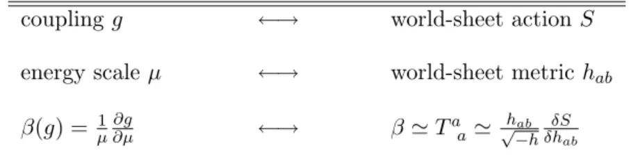
Quantum field theory String theory

couplingg ←→ world-sheet actionS

energy scaleµ ←→ world-sheet metric hab

β(g) = _µ1∂g_∂µ ←→ β 'Ta_a' _√hab −h

δS δhab

Table 2.1: analogy between renormalization functions in quantum field theory and string theory.

coupling parameter is described by what is called the renormalization β

function,

β(g) =µ∂g(µ)

∂µ =

∂g(µ)

∂lnµ. (2.2)

As can be seen from (2.2), when a theory is scale invariant, the β function should vanishes. When a β function does not vanish, it is said to have a

conformal anomaly.

One big difference between quantum field theory and string theory is the coupling. In quantum field theory, the coupling parameter depends on the energy scale. In string theory however, (as we will see in chapter 6) the coupling will become a spacetime dependent function, namely the exponent of a scalar field, eΦ(X).

Another big difference between quantum field theory and string theory is the meaning of theβ function. As we said before, in quantum field theory it is the dependence of the coupling on the energy scale. In string theory, however, it is the dependence of the action on the local world-sheet scale.

We can perform a conformal transformation, locally rescaling the world-sheet metric (see (1.9a)). Conformal invariance is a fundamental symmetry of string theory. This means that (at least classically) there is no confor-mal anoconfor-maly when we rescale the world-sheet metric, and therefore theseβ functions should vanish. Since the variation of the world-sheet action, with respect to the metric is proportional to the energy-stress tensorTab, we can see the analogy between β functions in quantum field theory and in string theory (see table 2.1). The importance of β functions will become clear in subsequent sections.

2.2 Weyl invariance and Weyl anomaly

2.2.1 Weyl invariance

Weyl transformations locally rescale the world-sheet by an overall factor. As we saw in section 1.3, only in two dimensions can a theory be conformal

(36)

invariant. Let’s investigate the property of Weyl invariance a bit further. An infinitesimal Weyl transformation (see (1.9a)) says that locally

hab−→hab+δhab (2.3a)

=hab+ 2habδω. (2.3b)

For the action to be Weyl invariant, we need the variation of the action with respect to the metrichab to vanish, so

δS δhab

= 0. (2.4)

According toNoether’s theorem the energy-stress tensor is written as (1.12). From this we see that the energy-stress tensor and the claim for Weyl in-variance are closely related. Actually the claim for Weyl inin-variance can be put in form Ta_a(σ) = p 4π −h(σ) δ δhab(σ) S hab(σ) (2.5a) = 0. (2.5b)

In other words, Weyl invariance implies the energy-stress tensor to be trace-less.

2.2.2 Path integral approach

However, this derivation is only true classically. In order to include quantum corrections, we need a different way of introducing the energy-stress tensor. Therefore, consider the path integral

Z ' Z

[dX] exp(−S[X, h]). (2.6)

This path integral counts the number of field configurations on the world-sheet. However, there is a huge set of configurations that only differ by a Weyl or diff transformation, and therefore render the same action. There-fore, there is an enormous overcounting of field configurations in this path integral. What we really want is the path integral, divided by the volume of the Weyl× diff symmetry group, Vdif f×W eyl. So we need to gauge fix the

path integral.

The way to do this is to choose a path trough the volume of the symmetry group, in such a way that each slice that represents the same theory is only crossed once. A way to carry out such a gauge fixing is known as the

Faddeev-Popov procedure, which is explained nicely in [11]. We will not go into detail here, but simply state that it comes down to introducing two new

(37)

2.2 Weyl invariance and Weyl anomaly 19

(anticommuting) Grassmann ghost fields, ca and bab and writing down an

action for these fields of the form, Sg =

1 2π

Z

d2σ√−hbab∇acb, (2.7)

where hab is now some fixed metric. Then the gauge fixed Polyakov path integral is locally written as

Z = Z [dX db dc] exp(−S[X, b, c, h]) (2.8a) = Z [dX db dc] exp(−S[X, h]−Sg). (2.8b)

This gauge fixed path integral can be used for calculating correlation func-tionsh. . .i_h, where

h. . .ih ≡

Z

[dX db dc] exp(−S[X, b, c, h]). . . . (2.9) Most of the time we will omit the discussion on ghosts in this thesis for the sake of simplicity, but formally they need to be included.

With this correlation function, we are able to deduce another expression for the energy-stress tensor. The way to do this is to vary this correlation function with respect tohab. When we do so and rewrite (1.12) as

δS δhab(σ) = p −h(σ) 4π T ab₍_σ₎_, _(2.10)

we see that this variation can be written as1

δh. . .i_h =− 1 4π Z d2σp−h(σ)δhab(σ) D Tab(σ). . .E h. (2.11)

So, the energy-stress tensor can be written as the infinitesimal variation of the path integral with respect to the metric.

This result is derived for general variations of the world-sheet metric. However, we are interested in the specific case where the variation was a Weyl variation. Therefore we can substitute (2.3b), i.e. δhab = 2habδω.

Performing a Weyl transformation and using (2.11), the expression for Tab becomes δWh. . .ih =− 1 2π Z d2σp−h(σ)δω(σ)hTa_a(σ). . .ih. (2.12) 1

From a mathematical point of view, the path integral (or partition function) (2.8b) can be seen as a functionalZˆ

S[hab(σ)]

˜

. Varying this functional with respect tohabrequires

applying the chainrule for functionals. With this procedure, we also need to integrate over the parametersσa_{, a}_{= 0}_,_{1. This explains the extra surface integral.}

(38)

2.2.3 Critical dimension

As we said before, demanding our theory to be Weyl-invariant now requires that the energy-stress tensor is traceless. So classically

Ta_aclassically= 0. (2.13) However, quantum effects can contribute to the trace of the energy-stress tensor, causing a conformal anomaly, or Weyl anomaly to occur. We have already investigated this property in chapter 3. One can show that (see [11]) the Weyl anomaly is equal to

hTa ai

QM

= − c

12R, (2.14)

wherec is called the central charge (which will be introduced in chapter 3) andR is the world-sheet Ricci scalar.2 The only way to obtain a consistent theory is if the total central charge isc= 0.

The central charge is made up of two components, namely the Xµ

bosonic field contributions cX and the ghost contributions cg. It can be shown the central charge for the ghost fields is cg = −26. Furthermore, every bosonic spacetime coordinate field Xµ _{contributes an amount of +1}

to the central charge. Therefore, we find that the total central charge is

c=cX +cg =D−26. (2.15)

So, Weyl invariance can only be achieved for D=Dc = 26, where D is

the number of spacetime fields Xµ, and therefore equal to the number of dimensions. This is the famous result that bosonic strings can only live in 26 dimensions.3 A bosonic string theory inDc = 26 is called acritical (bosonic) string theoryand for a critical string,Dcis called thecritical dimension. One

can also consider string theories with fermions, calledsuperstring theories. It turns out that the critical dimension for superstrings in flat spacetime is Dc = 10, as can be showed in quite a similar way.

In the derivation above we considered a string theory in flat spacetime. In a little while we shall include other backgrounds in our theory and see that this has a big influence on the condition for Weyl invariance. As we will see, the number of spacetime dimensions the strings lives in will be able to deviate from the critical dimension!

2

The Ricci scalar basically tells you how much curvature there is locally. For a non-flat world-sheetRgenerally is non-zero. Also see section B.

3

Note however, that have just looked at flat spacetime here! The metric is equal to the Minkowski metricηµν and no other background fields are involved.

(39)

2.3 Fields and target space 21

2.3 Fields and target space

When looking at string theory, it’s important to be aware of the similarities and differences between string theory and ordinary quantum field theory for point particles. For one, a classical point particle carves out a worldline, which can be parameterised by a parameterτ, and can be set equal to the particle’sproper time (see section 1.2). We can write down an action for a point particle, from which we can derive it’s equations of motion. A particle in quantum field theory is described by quantum fields φ(xµ), µ= 0, . . . ,3, living in D = 4 dimensions. A theory of these particles can be described by an action, involving the fields and derivatives of these fields. The four dimensions quantum fields live in, are equal to our spacetime. When we want to describe particles interacting with each other, we write down an action, involving the fields and derivatives, plus higher order terms and corresponding couplings.

This is not the case in string theory. First of all, strings are one-dimensional objects embedded in D spacetime dimensions. These strings are not generated by fields, as in quantum field theory. It is, however, pos-sible to define a field theory for strings. Such a theory is calledString field theory.4 You could say that string theory relates to string field theory as a point particle does to quantum field theory.

In contrast to the point particle, a string has infinitely many more in-ternal degrees of freedom, the oscillator modes, or string modes. These string modes can be seen as waves propagating on the world-sheet at the speed of light. When we quantize the string, the string modes actually be-come quantum modes of a two dimensional quantum field theory. Since a string propagates in D spacetime dimensions, there are D such fields Xµ(τ, σ), µ= 0, . . . , D−1. From the world-sheet’s point of view, the fields Xµcan be seen as the coordinates of a manifold, calledtarget space. In the case of string theory this is just equal to spacetime.

So particles in quantum field theory are described by quantum fields, living inD= 4 dimensions. Interactions can be described by putting higher order terms in the Lagrangian. Particles in string theory are described by different modes of a string propagating in spacetime. From the world-sheet’s point of view, a string mode is some configuration of D two dimensional quantum fields, which are embedded in spacetime.

In the next chapter we will study conformal field theory. Since the two-dimensional string world-sheet is conformal invariant, it is not a bad idea to

4

In string field theory there are fields Φ[X(σ)] which create and annihilate strings in a certain configuration. However, such fields do not even live in ordinary spacetime anymore, but in some sort of ‘stringy’ target space. It is possible to write down an action for open string field theory, but it turns out to be very complicated, if not impossible, to write down an action for closed string fields. This subject is, however, far beyond the scope of this thesis.

(40)

investigate this property to full extent. Conformal field theory provides us with a good way of achieving this. After having studied the mathematical framework of conformal field theory, we will incorparate it into a theory of interacting strings.

(41)

Chapter 3

Conformal field theory

3.1 Complex coordinates

3.1.1 Wick rotation

Conformal field theory is a very important tool for string theory. Interac-tions between strings and other strings, or backgrounds can be very hard to describe if one would try to parameterize the theory, and apply correct boundary conditions. An important idea that has been put forward is that interactions (for example the emission or absorption of strings) should be transformed (rescaled) in such a way that they become ‘pointlike’ opera-tors on the world-sheet. Since the world-sheet is conformal invariant, such transformations leave the theory unchanged. After having applied these transformations, it becomes very interesting to see how these operators be-have in the vicinity of each other. When two operators approach each other on the world-sheet, the quantum effects become apparent. A very conve-nient setting in which to study these sorts of interactions is calledconformal field theory (CFT). CFT is a very extensive subject, so we will just cover some bacis properties and give a global overview on the subject.

It turns out to be convenient to study interacting strings in a Euclidean framework, hab = δab. A Euclidean metric can easily be obtained by

per-forming aWick rotation on one of the world-sheet coordinates (usually the propertime coordinate).1 So we let

w=σ0+σ1 (3.1a)

=σ1+iσ2, (3.1b)

and w¯=σ1−iσ2. (3.1c)

It is easily checked that with these coordinates, the world-sheet metric in-deed has a Euclidean signature.

1

One has to be careful that when performing a Wick rotation, no poles are crossed. In most examples, however, this is not the case.

(42)

σ0 σ1 σ0 σ0 0 σ 0 σ0₀ σ0

Figure 3.1: Left: The world-sheet of a closed string is a cylinder in space-time. Right: The conformal mapping to complex coordinates. In the complex plane, the origin corresponds to the string’s proper time at minus infinity,

σ−∞0 . Points at |z| = ∞ correspond to the string’s proper time at plus

infinity,σ0∞

3.1.2 Conformal transformation

The next convenient choice is to perform a conformal transformation on these coordinates, such that

z=e−iσ1+σ2 (=e−iw) =z1+iz2, (3.2a) ¯

z=eiσ1+σ2 (=eiw¯) =z1−iz2. (3.2b) Both open and closed strings can be studied in these coordinates. However, since closed strings are most easily described in this setting, we will focus on them for the remainder of this chapter.

As we discussed before, the world-sheet of a closed string is a cylinder, where the string’s proper timeσ0 runs from −∞ to +∞, and the σ1 coor-dinate runs from 0 to 2π. In our new z coordinates, however, the string’s proper time runs radially outwards, withz= 0 corresponding toσ0 _{→ −∞}_,

and |z| → +∞ to σ0 → +∞. The σ1 coordinates at a fixed time σ2 are represented by circles around the origin. See figure 3.1.

Derivatives on the complex plane are defined by ∂≡∂z= 1 2(∂z1 −i∂z2), (3.3a) ¯ ∂≡∂¯z= 1 2(∂z1 +i∂z2), (3.3b)

(43)

3.2 Operator-product expansions 25

and in general, vectors with lower and upper indices transform as

(V1, V2)→(Vz, Vz¯), (3.4a) (Vz, Vz¯) = 1 2(V 1₊_iV2_{, V}1₋_iV2₎_, _(3.4b) and (V1, V2)→(Vz, Vz¯), (3.4c) (Vz, Vz¯) = 1 2(V1−iV2, V1+iV2). (3.4d) With these new coordinates, the metric also transforms. By working out the details, we findgzz =g¯zz¯= 0 and gzz¯=g¯zz = 1₂. Therefore, the inverse

of the metric gives gzz =gz¯z¯= 0 and gz¯z=gzz¯ = 2.2

3.2 Operator-product expansions

3.2.1 Currents and charges

On the world-sheet, one often encountersconserverd currents Ja, implying that ∂aJa = 0, and conserved charges Q, implying that _dtdQ = 0. A

con-served current induces a concon-served charge. By applying Gauss’ divergence theorem, one can show that the conserved charge on the world-sheet, induced by a conserved current equals

Q= 1 2π

Z 2π

0

dσ1J0. (3.5)

Next, we can switch to complex coordinates (w,w¯), and Wick rotate J0 = iJ2. In this case, the integral splits up into a holomorfic part (only dependent onw) and aanti-holomorphic part (only dependent on ¯w). Then, we can switch to the conformally transformed coordinates (z,z¯) and see that the integrals turn into contour integrals around the origin.

We know fromNoether’s theorem that every symmetry of an action gives rise to a conserved current. We will use this to study the conserved current for conformal symmetry. Fist of all, consider the energy-stress tensor on the world-sheet, Tab. We already discussed that the energy-stress tensor itself is conserved, meaning ∂aTab = 0. Then, moving to the complex plane, it

can be shown that this leads to the conditions

∂z¯Tzz = 0, → Tzz =T(z), (3.6a)

∂zT¯zz¯= 0, → T¯zz¯= ¯T(¯z), (3.6b)

soT(z) is holomorfic, and ¯T(¯z) is anti-holomorfic.

This derivation works quite similar for the current of conformal symme-try, Ja() = Tabb, where b is an infinitesimal conformal transformation.

(44)

If (z) and ¯(¯z) represent infinitesimal conformal transformations on the complex plane, the current Ja() also splits up into a holomorfic and

anti-holomorfic part,

Jz =T(z)(z), (3.7a)

Jz¯= ¯T(¯z)¯(¯z). (3.7b)

In the following we will show how this can be used to generate conformal transformations of fields, living on the complex plane.

3.2.2 Generators of conformal transformations

In quantum field theory one often needs the product of two (or more) opera-tors, for example when calculating correlation functions. But such a product only makes sense if it is time-ordered.3 Since the world-sheet’s proper time coordinate of a (closed) string in conformal complex coordinates runs radi-ally outwards, we imposeradial ordering for operator products, i.e.

RA(z,z¯)B(w,w¯) =

A(z,z¯)B(w,w¯) for|z|>|w|

B(w,w¯)A(z,z¯) for|z|<|w| . (3.8) Now we turn our attention back to the conserved charge for conformal transformations, Q. Such a charge can generate (infinitesimal) conformal

transformations. The quantum version of an infinitesimal conformal trans-formation of a fieldφ(z,z¯) is given by the commutator with Q, i.e.

δφ(z,z¯) = [Q, φ(z,z¯)] (3.9a)

= 1

2πi I

du (u) [T(u)φ(z,z¯)−φ(z,z¯)T(u)], (3.9b) where we have just written down the holomorphic part here. The anti-holomorphic part is written is a similar way. But as we just discussed with radial ordering, the first term only makes sense for|u|>|z|, and the second term only makes sense|z|>|u|. Since these contour integral are integrated along contours around the origin, we can deform these contours in such a way that we end up with just one contour around the pointz,γz (see [12]

for a more detailed derivation). So, therefore the variation of a fieldφ(z,z¯) can finally be written as

δφ(z,z¯) = [Q, φ(z,z¯)] (3.10a) = 1 2πi I γz du (u)R(T(u)φ(z,z¯)). (3.10b)

3_{Time ordering makes sure that the operators are put in the correct order. If this is}

not the case, one can have a situation where the expectation values of the product blow up, and would therefore be undefined.