Data Analysis and Reporting
in GMP DWH
Jiří Jarkovský, Jiří Kalina, Ladislav Dušek, Jana Klánová,
Richard Hůlek, Daniel Klimeš, Daniel Schwarz, Petr Holub,
Jakub Gregor, Jana Borůvková, Kateřina Šebková
1
Contents
1 Introduction – guide to chapters ... 2
2 Technical note on statistical analysis in GMP ... 4
2.1 Introduction ... 4
2.2 General principles ... 4
2.2.1 Data pre-processing ... 4
2.2.2 From primary to aggregated POPs concentrations ... 5
2.2.3 Statistical testing and its power ... 5
2.2.4 Exploratory and confirmatory statistics: estimates and comparisons ... 5
2.3 Proposed outcomes of the statistical processing of GMP data ... 6
2.3.1 Summary statistics POPs concentrations in the atmosphere ... 6
2.3.2 Uncertainty analysis ... 6
2.3.3 Power analysis: quantification of minimum detectable difference ... 7
2.3.4 Stochastic identification of time trends ... 7
2.3.5 Quantification of time trends ... 7
2.4 References ... 8
3 Evaluation of atmospheric concentrations of selected POPs from GMP 1 data collection campaign – content analysis ... 9
3.1 Available data in GMP 1 database ... 9
3.2 Six levels of data selection ... 12
3.3 Statistical methodology ... 13
3.4 Results – air monitoring using passive sampling ... 17
3.5 Results - air monitoring using active sampling ... 20
4 Reporting of GMP data collected in the period 1998-2008 and its extension ... 25
4.1 World map – monitoring overview ... 25
4.2 Available data – parameters ... 26
4.3 Available data – years ... 26
4.4 Reported values – summary statistics ... 27
4.5 Reported values – advanced interactive map visualization ... 27
4.6 Time series analysis ... 27
2
1
Introduction – guide to chapters
The statistical methodology and data processing in GMP 2 is based on the approaches adopted for the data analysis in GMP 1 with new improvements and extensions. These extensions aim at trend comparison. The standards and principles adopted from the GMP1 are shown in the following chapters:
- Technical note on statistical analysis in GMP
- Evaluation of atmospheric concentrations of selected POPs from GMP 1 data collection campaign – content analysis
New improvements and annexes of proposed methodology in data analysis are summarized in chapters:
- Reporting of GMP data in 1998-2008 and its extension - Documentation of new GIS module for GMP DWH
The robust design of methods allows the use of the set of algorithms to any GMP data collection campaign records. It can also include subsequent campaigns, comparison and testing of time series. The methodology supports the following tasks:
- Validation and description of data availability - Summary statistics of reported concentration values
- Visualization of reported concentration values using a novel GIS map technology
- Complex time series analysis of POPs concentrations and confirmatory assessment of time-related changes in contamination
- All outcomes of statistical processing are generated in user friendly interactive reports, fully accessible on-line
3
4
2
Technical note on statistical analysis in GMP
(published in “Guidance on the global monitoring plan for persistent organic pollutants”, document UNEP/POPS/COP.6/INF/31, version January 2013).
2.1
Introduction
The aim of this technical note is to complement the statistical methodology published in earlier version of the GMP Guidance Document, and to specify methodical procedures which should be employed when processing POPs data reported to the GMP. Based on the practical experience with the first GMP reports data processing, this technical note specifies obligatory data fields which should be filled in order to allow correct interpretation of the data analysis. Finally, this text highlights the most important data pre-processing and processing steps and proposes a logical sequence of the statistical outcomes. The methodology is based on robust statistical methods which can be generally applied for statistical analysis of POPs concentrations in any environmental matrix reported in GMP 2 (air, human tissues, water).
2.2
General principles
2.2.1 Data pre-processing
Correct definition of data is an unavoidable prerequisite of all subsequent statistical analyses. Only reliably reported concentration values can be accepted for any spatial or temporal comparisons. Therefore, a multilevel evaluation procedure based on the annually aggregated concentrations is proposed to maintain a high predictive value of the GMP records while avoiding bias in the concentration values.
The evaluation of the first GMP reports revealed a number of challenges related to data standardization, such as the lack of a standardized taxonomy for the listed POPs, their isomers, transformation products and summations. Some records provided detailed primary data, including rarely measured compounds, while others contained only the sums of the key groups of POPs. The data heterogeneity was further enhanced by reporting various toxic equivalents (TEQ) (based on the WHO TEF values from different years) rather than concentrations of each PCDDs, PCDFs and PCB congener. Unclear identification of matrices, units, time scales of reported concentrations, as well as insufficient specification of aggregated data have also been observed. Large volumes of valuable data have been generated in all regions and further standardization of reporting formats would significantly improve their applicability. A more elaborated guidance for handling, reporting and
analyzing/interpreting these data will thus improve their applicability and support the development of the second GMP reports.
The practical experience with processing and validation of GMP1 records established more precise data handling rules for the future data collection. The rules define mandatory data fields which correspond to the standardized structure of the GMP DWH: typology of the background site; definition of the matrix; taxonomy of parameters; sampling frequency (and data aggregation, if applied) and measured value specified by its unit and data variability.
The proposed data evaluation procedure guarantees comparability of the different samples, taking into account type of site, matrix, sampling method, time span and sampling frequency. Heterogeneity in these factors might a dramatically increase the uncertainty in the final outcomes. The pre-processing
5
procedures also limit the impact of uncontrolled covariates and thus reduce the risk of false trend detection or the risk of neglecting truly significant changes.
a) Initial data filtering stratifies the records according to objective entities, such as site-matrix type and analyzed compounds. The filters must also check/verify the completeness of the primary GMP DWH database records in the reported sampling frequency, number of detected LOQs and their handling rules.
b) In the statistical part, the validation procedure excludes obvious extreme or unreliable values from quantitative analyses. The outlying concentrations can be identified by checking their quantile position in the sample distribution function. Estimated mean and standard deviation of log transformed annually aggregated data can be used for the reconstruction of the normal or log-normal distribution; a resulting pattern can be used to assess probabilistic position of the point values.
2.2.2 From primary to aggregated POPs concentrations
Seasonal dynamic is the most important source of variability in levels of POPs concentrations measured in the atmosphere s. This is not the case for human tissue data. Provided that primary concentration data sets (atmosphere) are available, the impact of seasonality can be quantified and extracted from the time series by proper smoothing techniques and adjusting statistical models. Seasonally-adjusted time series constitute a pool for the subsequent trend detection and quantification. Annually aggregated data can also be used for spatial and temporal comparisons and quantification of time-related trends. Most records reported to the first GMP data collections are annually aggregated arithmetic means. Nevertheless the experience shows that the aggregated values must be reported with appropriate variability estimates generated from primary data in the future (5th-95th percentile range and standard deviation are recommended). The quantity of non-detects (below LOQ values) in the primary records and their handling in the mean calculations must be provided as well.
2.2.3 Statistical testing and its power
Power analysis is an obligatory step to define reliably the magnitude of changes identified by the statistical methods. Power analysis minimizes the risk of misinterpretation or of the incorrect generalization on the basis of values observed. The power calculation must be applied for both the statistical trend detection (Mann-Kendall algorithms) and the quantification (paired tests assessing the difference in the annual arithmetic or geometric means). Two approaches are recommended for GMP data testing, in particular, for the time trend detection:
a) Quantification of the minimum detectable difference between the annually aggregated values allowing to benchmark the identified changes against the statistically detectable levels; b) Prospective calculation of the sample size needed for the detection of a given relative time
change in the POPs concentrations (e.g. 50% annual decrease).
2.2.4 Exploratory and confirmatory statistics: estimates and comparisons
Simplicity and robustness are the main principles when processing the GMP records. Non-parametric tests and summary statistics without or with negligible assumptions for the distribution patterns are highly recommended:
- Median estimates supplied with a 5th-95th percentile range and geometric mean estimated on the basis of log-transformed data with a corresponding 95% confidence interval are
6
recommended for the summary statistics. Mann-Kendall U test, Kruskal-Wallis test, and Wilcoxon paired rank sum test are recommended for comparative analyses.
- Spearman’s rank correlation coefficient is recommended for correlation analysis.
2.3
Proposed outcomes of the statistical processing of GMP data
The following outcomes are proposed for the statistical processing of GMP data: 1) Summary statistics of POPs concentrations in the atmosphere
2) Uncertainty analysis
3) Power analysis: quantification of the minimum detectable difference as a base for relevant estimates of changes over time and, if possible, of time trends
4) Stochastic identification of time trends 5) Quantification of time trends
2.3.1 Summary statistics POPs concentrations in the atmosphere
Annually aggregated POPs concentrations, calculated as arithmetic means from the primary values can be used for both the quantitative and qualitative analyses (see also section 2.2). In order to evaluate the heterogeneity of the primary data, the individual compounds values have to be assessed for their sample size and type of data sources. Two approaches are recommended for assessing summary statistics of the concentration values:
a) Median estimate reported together with a 5th-95th percentile range
b) Geometric mean estimate based on the log-transformed annual averages with a corresponding 95% confidence interval
The variability of the baseline values can be evaluated at local, regional or global scale, merging appropriate data sets. The underlying data pooling (both primary and aggregated data), however, has to be supported by an uncertainty analysis (see 3.2).
Non-parametric tests like Mann-Kendall U test or Kruskal-Wallis test are recommended for
interregional comparison of POPs concentrations. Parametric test like ANOVA models or analysis of covariance can be applied only after an effective normalizing transformation of the concentration estimates.
2.3.2 Uncertainty analysis
Data reported to the GMP are generated by a variety of programmes, at several background sites of each UN region; therefore, they have to be inspected for an intra-regional and inter-regional
homogeneity in the annually averaged POPs concentrations. Graphically, regional variability can be reported as the intra-regional 5th-95th percentile range. Sample distribution functions of the regional samples can then be compared and tested by proper robust methods (Kolmogorov-Smirnov test, Kruskal-Wallis test). The same applies to geometric means of the averaged concentrations and their 95% confidence intervals.
The uncertainty analysis identifies regions or data subsets with an increased intra-regional variability in the annually averaged concentrations as well as sources of such variability (evident outlying values should be excluded). Any spatial or temporal comparison should be preceded by an assessment of internal homogeneity of concentration values in the areas of interest.
7
Similarly, the homogeneity should also be assessed in the time trend analysis (i.e. presence of and same direction in the trend change and annual difference). A year-to-year difference can be compared among time-series based on the individual sites. Such variability can be expressed as a standardized year-to-year difference or as a coefficient of variation (expressed in %). Applying time-related regression models and their residuals is possible as well. In the existing time series, homogeneity (or non-homogeneity) in a year-to-year variance indicates the degree of representativeness and the stability of identified time trends. The time series reported from various sites can be merged for more powerful trend analysis only if their homogeneity was confirmed.
2.3.3 Power analysis: quantification of minimum detectable difference
The heterogeneity and a limited accessibility of primary data in the first GMP reports significantly limit the power analysis of time trends for many compounds. Time-related analysis performed on the annually aggregated data (see 2.2) partially reduces their sensitivity and the ability to detect significant differences. Therefore, any time trend analysis must be accompanied by power analysis, and the identified trends must always be reported together with the corresponding minimum detectable difference. Power analysis estimates a minimum difference between the two annually aggregated concentration values detectable by paired t-test on log-transformed data (α = 0.05 and β = 0.20).
Appropriate non-parametric alternatives such as the Wilcoxon-rank-sum test or the Mann-Kendall test can be used as well, especially in cases where the analysis is based on primary concentration data rather than on normalized data. This approach should be tested in a pilot study performed on available primary data sets at first.
2.3.4 Stochastic identification of time trends
Time trends are identified via a qualitative test for a statistical significance of the time-related changes observed in the consecutive measurements. At least five consecutive annually aggregated
concentration values are required when assessing time trends using one of the following robust techniques:
- The Daniel’s test, as an application of the Spearman’s rank correlation coefficient between the concentration values and corresponding time ranks;
- The Mann-Kendal test, as a non-parametric test for detecting a trend in time series, based on binary coding of the changes in measurements consecutive in time.
The direction of the time trend (whether concentration values are increasing or decreasing over time) has to be recorded whenever it is confirmed as statistically significant. In addition, any concentration change over time should be reported in the same way, although there is no exact statistical significance behind it. Both the statistically significant and the non-significant time changes over time must be correctly quantified in the reports and marked with the p value generated by appropriate tests (see 2.3.5).
2.3.5 Quantification of time trends
A quantification of time trends should be performed whenever the proper statistical tests confirm significant and consistent time-related differences in POPs concentrations (see 3.4). A quantified trend
means a difference Δ=y1–y2, where y1 and y2 correspond to annually aggregated concentration values
recorded in two consecutive years. The time-related difference in the concentration value should be expressed with the following attributes:
- The difference as an absolute value expressed in concentration units;
8
- The 95% confidence interval of the time-related difference; - The p value of the trend test;
- The corresponding minimum detectable annual difference.
In addition, it can be useful to monitor temporal changes of relative contribution, together with the evaluation of the temporal changes in POPs concentrations in core matrices. Such information can provide a new insight into the changing primary and secondary sources or to the transport pathways of POPs.
2.4
References
- Bails, D. G. and Peppers, L. C. (1982) Business fluctuations: Forecasting techniques and applications. Englewood Cliffs, NJ: Prentice-Hall.
- Cohen, J. (1988). Statistical Power Analysis for the Behavioral Sciences (second ed.). Lawrence Erlbaum Associates, Hillsdale, New Jersey.
- Daniels, H.E. (1950) Rank correlation and population models. Journal of Royal Statistical Society Series B, 12, 171–181.
- Hirsch, R.M., Slack, J.R. and Smith, R.A. (1982) Techniques of Trend Analysis for Monthly Water Quality Data, Water Resources Research 18(1), 107-121.
- Holoubek, I; Klanova, J; Jarkovsky, J; Kohoutek, J (2007) Trends in background levels of persistent organic pollutants at Kosetice observatory, Czech Republic. Part I. Ambient air and wet deposition 1996-2005. Journal Of Environmental Monitoring. 9 (6), 557-563.
- Kendall, M.G. (1975) Rank Correlation Methods, Charles Griffin, London.
- Libiseller, C. and Grimvall, A. (2002) Performance of Partial Mann-Kendall Test for Trend Detection in the Presence of Covariates. Environmetrics 13, 71-84.
- Libiseller, C. (2004) MULTMK/PARTMK – A program for the computation of multivariate and partial Mann-Kendall tests. http://www.mai.liu.se/~cllib/welcome/PMKtest.html.
- Limpert, E.; Stahel, W.; Abbt, M. (2001) Log-normal Distributions across the Sciences: Keys and Clues. BioScience. 51 (5), 341–352.
- Mann, H.B. (1945) Nonparametric tests against trend. Econometrica 13, 245-259. - Shasha, D. (2004), High Performance Discovery in Time Series, Berlin: Springer.
- Wei, W. W. (1989). Time series analysis: Univariate and multivariate methods. New York: Addison-Wesley.
- Zar, J.H. (2009) Biostatistical Analysis (5th Edition). Prentice Hall, Upper Saddle River, New Jersey 07458.
9
3
Evaluation of atmospheric concentrations of selected POPs from GMP 1
data collection campaign – content analysis
3.1
Available data in GMP 1 database
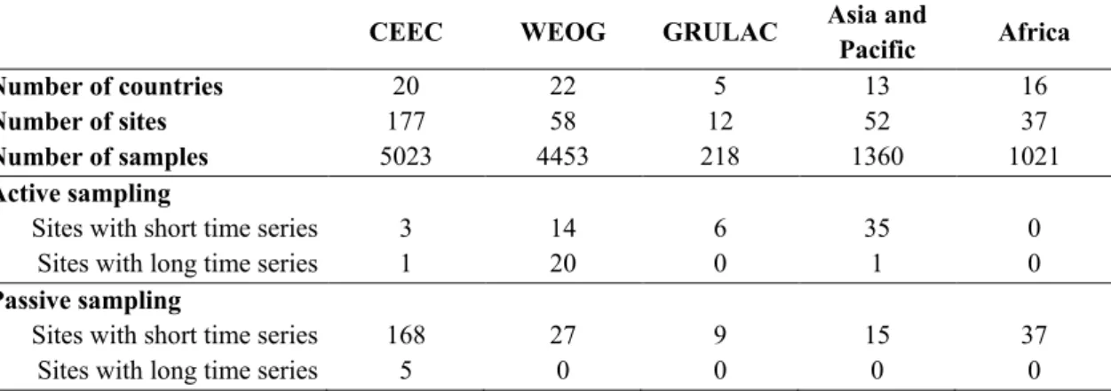
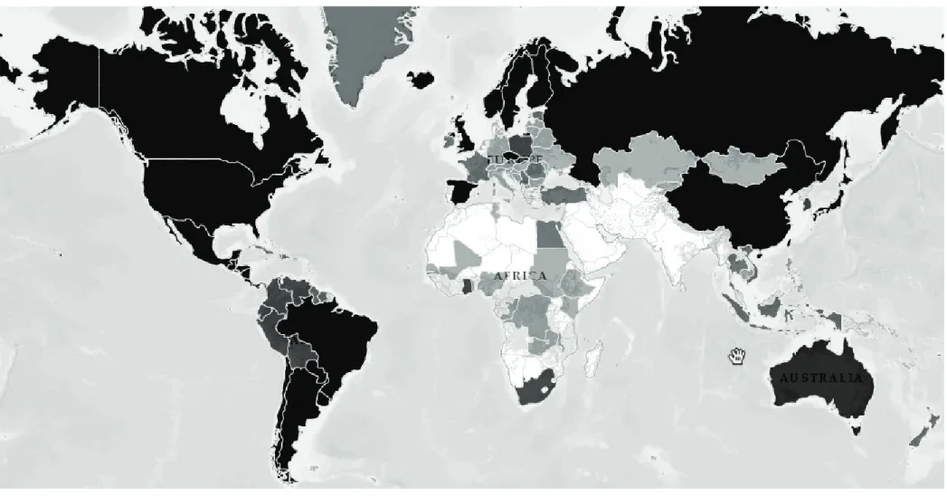
The GMP 1 data repository aggregates air pollution data from multiple sources covering 177 POPs compounds (Tables 1 and 2) from 76 countries (Figure 2). The number of countries, sites and measurements are summarized in Table 1.
Table 1. Countries, sampling sites and samples from air monitoring in the five UN regions (samples are aggregated annually)
CEEC WEOG GRULAC Asia and Pacific Africa
Number of countries 20 22 5 13 16
Number of sites 177 58 12 52 37
Number of samples 5023 4453 218 1360 1021
Active sampling
Sites with short time series 3 14 6 35 0
Sites with long time series 1 20 0 1 0
Passive sampling
Sites with short time series 168 27 9 15 37
10
11
12
3.2
Six levels of data selection
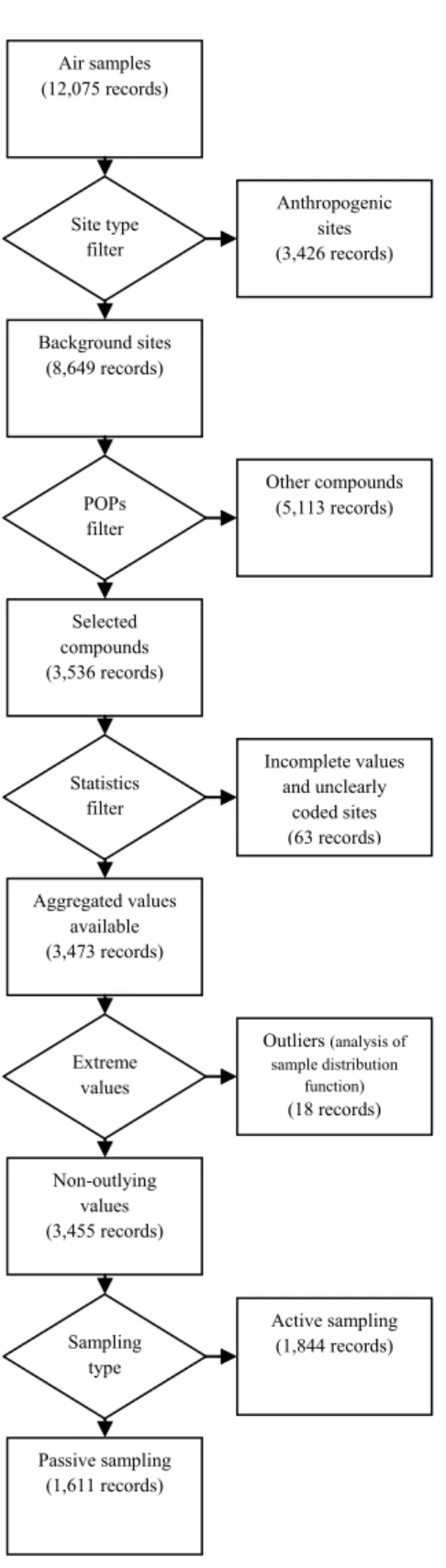
For a reliable assessment of the baseline POPs concentrations, a six-step validation procedure was applied on the annually aggregated GMP1 data. This procedure was introduced in order to maintain a high predictive value of the GMP1 records and to avoid bias in the concentration values.
The initial data filtering stratified the records by objective entities such as the sampling matrix, site type and compounds analyzed, and subsequently excluded apparently extreme or unreliable values from the quantitative analysis.
This case study is focused on POPs concentrations in ambient air. Other matrices reported in GMP1 - breast milk and blood – were not included. Therefore, in the first step, only 10,216 records resulting from atmospheric monitoring were used from a total of 16,317 records.
The second validation step verified the relevance and
completeness in the identification of the sampling site (spatially aggregated atmospheric samples were excluded, except for the GRULAC region, where they were aggregated over the remote background sites). The subsequent analysis considers only clearly coded background sites: sampling sites with increased pollution stemming from industry, transport or agricultural production were filtered out. These controls resulted in a smaller sub-set of 7,120 records provided from well-described background sites.
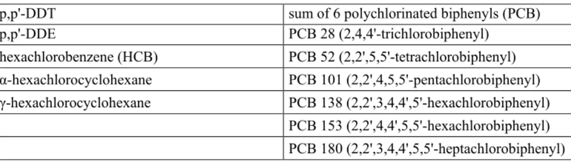
In the third step, the procedure separated 1,694 records of selected substances well-represented in GMP1 to estimate their concentrations. Among the initial 12 legacy POPs reported in GMP1, DDTs (p,p'-DDT and p,p'-DDE), hexachlorobenzene (HCB) and a sum of 6 polychlorinated biphenyls (PCBs) were selected. In addition, alpha-HCH and gamma-HCH from newly listed POPs were also reported frequently. Further selection was carried out according to the accessibility of time series data for pilot estimates of historical time trends and for changes over time. At least one time series with five consecutive years of measurement on one site was required for this purpose at a minimum. Such requirement was fulfilled for all of the 12 parameters (groups) listed in Table 1.
The fourth step – statistical filter - removed 85 records with the atmospheric concentration expressed by other statistical characteristic than the mean value of the measurements performed during the one-year period (i.e. percentiles, minimum, maximum, median estimates and values that covered unclear periods of time were excluded).
Figure 3. Six-step validation process of the GMP 1 records.
Air samples (12,075 records) Site type filter Background sites (8,649 records) Anthropogenic sites (3,426 records) POPs filter Other compounds (5,113 records) Selected compounds (3,536 records) Statistics filter Incomplete values and unclearly coded sites (63 records) Aggregated values available (3,473 records) Extreme values Outliers (analysis of sample distribution function) (18 records) Non-outlying values (3,455 records) Sampling type Active sampling (1,844 records) Passive sampling (1,611 records)
13
The fifth step excluded statistically verified extreme values, i.e. points exceeding the 95th percentile in a computer-assisted reconstruction of log-normal distribution of primary values.
The final pool of data consisted of 1,560 records that were classified according to the sampling method, i.e. active and passive samples. Statistical analysis was separately performed for these two groups.
Table 3. Parameters selected for the GMP 1 pilot analysis
p,p'-DDT sum of 6 polychlorinated biphenyls (PCB)
p,p'-DDE PCB 28 (2,4,4'-trichlorobiphenyl) hexachlorobenzene (HCB) PCB 52 (2,2',5,5'-tetrachlorobiphenyl) α-hexachlorocyclohexane PCB 101 (2,2',4,5,5'-pentachlorobiphenyl) γ-hexachlorocyclohexane PCB 138 (2,2',3,4,4',5'-hexachlorobiphenyl) PCB 153 (2,2',4,4',5,5'-hexachlorobiphenyl) PCB 180 (2,2',3,4,4',5,5'-heptachlorobiphenyl)
The compounds in Table 3 were included in the model training data set to demonstrate the validity of the proposed methodology. The selection of POPs for the analysis was based on the list of 12 initial POPs reported in GMP1 with respect to the availability of data. Furthermore, α-HCH and γ-HCH were also included, since the volume of GMP1data for these compounds was large enough to enable a reliable analysis.
3.3
Statistical methodology
The statistical analysis was carried out for 5 individual parameters listed in Table 1 and separately for the sum of the six indicator PCB congeners. Quantitative and qualitative analyses were performed solely on the annually aggregated concentration values reported in GMP1 or on obtained from GMP1 primary data by arithmetic mean. All statistical calculations were applied on the basis of standard and robust methods, without excessive requirements on the sample size or on the shape of sample
distribution of primary values.
The sample size and range of data sources were assessed for each parameter. This step is very important for clarifying the heterogeneity of the primary GMP1 records, as some compounds were reported from several regions/sites, while others were reported only from one site. The following descriptive items were evaluated and summarized:
- Data source: information on the site/laboratory/project reporting the data. In the case of a single source, this is directly identified. For a more robust estimation, data combined from several reporting units were taken; then the “multiple reports” code is used.
- Period: time span (in years) for which data assessment can take place.
- No. of records: sample size used for the calculation of the relevant statistical quantity. - Value: the value of the statistical quantity (e.g. quantified concentrations, time trend, etc.), if
available; otherwise the "N/A" code was used.
The following five statistical measures were examined as key endpoints:
1) Summary statistics of POPs concentrations. A robust set of descriptive statistics based on
14
a) Regional median supplemented by 5th and 95th percentile: computed for all records over
the accessible sampling period. This value describes the overall range of all values and serves as a robust description of the central tendency in the sample data distribution.
b) Regional geometric mean and its 95% confidence interval: computed over the accessible
sampling period. It provides a parametric estimate of the concentration based on the assumption of lognormal distribution of values.
c) Regional arithmetic mean: provides a supplementary description of the concentration values
in the region over the accessible sampling period. This procedure was used as a quantitative estimate, although the sample distributions do not correspond to the normal distribution model.
2) Detectable alternative for time trend estimates, expressed as the minimum detectable annual
difference, was estimated in available time series using power analysis for the minimum statistically significant detectable difference of two arithmetic means (annually averaged concentration values) in paired t-test with α = 0.05 and power = 0.80.
The difference between the start and the end of the series was computed, and t divided by the length of the time series, to obtain average annual differences for each site with at least two concentration values available. The standard deviation of the differences were used as input to the standard power analysis of the paired t-test together with a desired power = 0.80 (1 – β) andα =
0.05; the paired t-test was selected as a standard test for analysing the differences in the situation, where the computed differences follow a normal distribution; this was also valid for cases where primary concentration data were log-normally distributed.
The computation is based on the following formula:
N
SD
t
DA
=
1v−α/2×
where DA is estimated detectable alternative, SD represents the standard deviation of the differences, tν is value of Student’s distribution for a given power, α represents the degree of
freedom (n=ν-1).
3) Time trend identification, as a qualitative test which confirms a consistent time trend among the
consecutive POPs values in terms of the statistical significance. Robust Mann-Kendall tests were used. The evaluation was applicable only to those sites with at least five consecutive annually
aggregated mean concentration values available. α = 0.05 was used as a level of statistical
significance in all tests.
The Mann-Kendall test (Mann, 1945; Kendall, 1975) is a non-parametric test for identifying trends in data time series. The test compares relative magnitudes of sample data instead of the exact values. The main benefit of this test is that data do not need to conform to any particular
distribution. Moreover, data reported as not-detected can be included in the test by replacing them with a common value smaller than the smallest measured value in the data set. The procedure assumes that there is only one value per each point in time. The median is used for multiple data points over a single time period.
Data values are evaluated as sorted time series. Each data value is compared to all subsequent data values. The initial value of the Mann-Kendall statistics, S, is assumed to be 0 (e.g., no trend). If a
15
value from a subsequent time period is higher, the S is increased by 1. On the other hand, if the value in the following time period is lower than a value sampled earlier, S is diminished by 1. The net result of all such increments and decreases yields the final value of S.
Let x1, x2,…, xn represent n data points where xj represents the data point at time j. Then the Mann-Kendall statistics (S) is given by
∑ ∑
− = = +−
=
1 1 1),
(
n k n k j j kx
x
sign
S
where . 0 1 0 0 0 1 ) ( < − − = − > − = − k j k j k j k j x x if x x if x x if x x signA high positive value of S is an indicator of an increasing trend, and a low negative value indicates a decreasing trend. However, it is necessary to compute the probability associated with S and with the sample size, n, to quantify statistically the significance of the trend observed.
The variance of S is defined as
, ) 5 2 )( 1 ( ) 5 2 )( 1 ( 18 1 ) ( 1 + − − + − =
∑
= g p tp tp tp n n n S VARwhere n is the number of data points, g is the number of tied groups (a tied group is a set of sample data having the same value), and tp is the number of data points in the pth group. For example, in the model sequence {2, 3, non-detect, 3, non-detect, 3}, n=6, g=2, t1=2 for the non-detects, and
t2=3 for the tied value 3.
A normalized test statistic Z can be then computed as follows:
< + = > − = 0 ) ( 1 0 0 0 ) ( 1 S if S VAR S S if S if S VAR S Z
The trend is considered decreasing if Z is negative and the computed probability is higher than the level of significance. The trend is considered increasing if Z is positive and the computed
probability is higher than the level of significance. If the computed probability is lower than the level of significance, there is no trend.
Standardized version of statistic S, called Kendall tau is used for description of trends in Tables 3 and 5.
4) Time trend quantification is computed using a linear regression slope estimate. The quantified trend represents the mean annual change based on a linear model and supplemented by its 95%
16
confidence interval. Simple linear regression (Zar, 1998) for time series trend estimate is defined as:
i i
í
X
Y
=
α
+
β
+
ε
where α and β are constants and ɛi is referred to as an “error” or “residual”. The parameter β is also called the regression coefficient, the slope or the trend estimate in time series analysis and
parameter α is called Y intercept. If the estimate for β is b and for α is the best estimate a, then the sample regression equation is expressed as:
i
i
a
bX
Y
ˆ
=
+
The trend, b, of the regression line computed from sample data expresses quantitatively the straight-line dependence of Y and X in the sample. It is possible to obtain a sample of data points (i.e. by random sampling) where the calculated b would suggest that β was positive, even though it
is, in fact, zero. It is unlikely to obtain points to yield β=0 by a random sampling.
To demonstrate the likelihood, we can examine the null hypothesis
: 0
0H
β
=
, and the alternate hypothesis,:
β
≠
0.
AH
Thus, if the probability of obtaining the calculated b is small (let’s say 5% or less), then 0H
is rejected, and AH
is assumed to be true. This null hypothesis for β can be tested for example by using Student’s t statistic. The (1-α) confidence interval can be calculated for the parameter being estimated (β) using Student’s t statistic as:, ) 2 ( ), 2 ( n sb t b± α −
where sb is the standard error of b and is calculated using residual mean square, which is often written as 2 X Y
s
⋅ ,.
2 2∑
⋅=
x
s
s
YX bThe residual mean square depends on residual sum of squares and residual degree of freedom as follows
(
)
,
/
ˆ
2 2residualDF
residualSS
s
DF
regression
totalDF
residualDF
Y
Y
residualSS
X Y i i=
−
=
−
=
⋅∑
When working with a simple linear regression then the regressionDF equals 1 and the totalDF is
17
3.4
Results – air monitoring using passive sampling
Table 4 contains aggregated entries summarizing data sources for the statistical analysis performed, i.e. the sites where relevant passive sampling data were available. Subsequently to the six-step
validation, the entire data set consists of 1,279 entries from all five UN regions. The cell in the table is shaded if there were no data entries available.
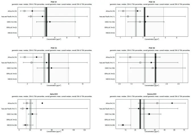
The statistical summary is complemented by the variability/uncertainty analysis as shown in Figure 2, consisting of six parts; each focusing on an individual parameter (compound) in the analysis.
The analysis compares median and geometric mean estimates and their variability among the individual UN regions. The boxes in the charts indicate medians and the circles geometric means of the data sets from the individual regions; whiskers correspond to the 5th–95th percentile range. The shaded area of the chart corresponds to the 5th – 95th percentile range of the entire set of sites for all regions; the grey vertical stripe corresponds to the global median estimate and the black vertical stripe corresponds to the global geometric mean estimate of this set.
Table 5 displays results of the statistical analysis of validated atmospheric POPs concentrations obtained by passive sampling.
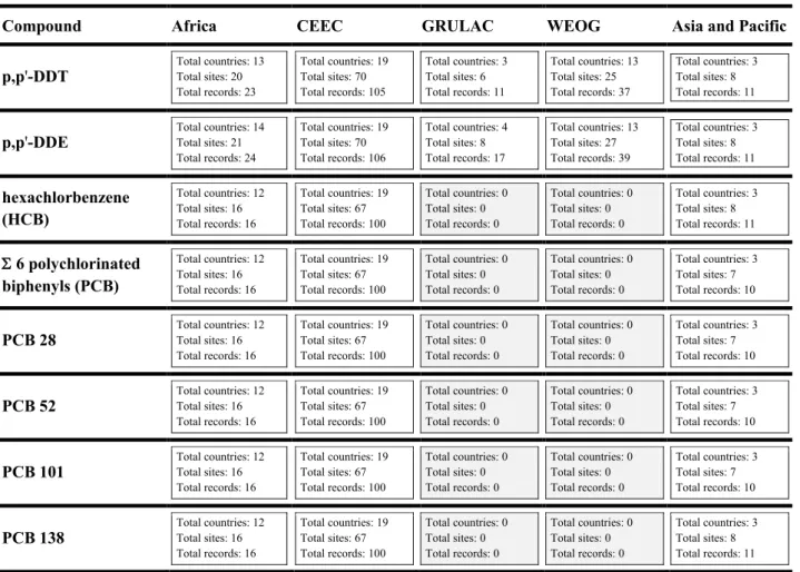
Table 4. Accessible data sources for air monitoring using passive sampling (if data entries from no site are available, the cell is shaded)
Compound Africa CEEC GRULAC WEOG Asia and Pacific
p,p'-DDT Total countries: 13 Total sites: 20
Total records: 23 Total countries: 19 Total sites: 70 Total records: 105 Total countries: 3 Total sites: 6 Total records: 11 Total countries: 13 Total sites: 25 Total records: 37 Total countries: 3 Total sites: 8 Total records: 11
p,p'-DDE Total countries: 14 Total sites: 21
Total records: 24 Total countries: 19 Total sites: 70 Total records: 106 Total countries: 4 Total sites: 8 Total records: 17 Total countries: 13 Total sites: 27 Total records: 39 Total countries: 3 Total sites: 8 Total records: 11 hexachlorbenzene (HCB) Total countries: 12 Total sites: 16 Total records: 16 Total countries: 19 Total sites: 67 Total records: 100 Total countries: 0 Total sites: 0 Total records: 0 Total countries: 0 Total sites: 0 Total records: 0 Total countries: 3 Total sites: 8 Total records: 11 Σ 6 polychlorinated biphenyls (PCB) Total countries: 12 Total sites: 16 Total records: 16 Total countries: 19 Total sites: 67 Total records: 100 Total countries: 0 Total sites: 0 Total records: 0 Total countries: 0 Total sites: 0 Total records: 0 Total countries: 3 Total sites: 7 Total records: 10
PCB 28 Total countries: 12 Total sites: 16
Total records: 16 Total countries: 19 Total sites: 67 Total records: 100 Total countries: 0 Total sites: 0 Total records: 0 Total countries: 0 Total sites: 0 Total records: 0 Total countries: 3 Total sites: 7 Total records: 10
PCB 52 Total countries: 12 Total sites: 16
Total records: 16 Total countries: 19 Total sites: 67 Total records: 100 Total countries: 0 Total sites: 0 Total records: 0 Total countries: 0 Total sites: 0 Total records: 0 Total countries: 3 Total sites: 7 Total records: 10
PCB 101 Total countries: 12 Total sites: 16
Total records: 16 Total countries: 19 Total sites: 67 Total records: 100 Total countries: 0 Total sites: 0 Total records: 0 Total countries: 0 Total sites: 0 Total records: 0 Total countries: 3 Total sites: 7 Total records: 10
PCB 138 Total countries: 12 Total sites: 16
Total records: 16 Total countries: 19 Total sites: 67 Total records: 100 Total countries: 0 Total sites: 0 Total records: 0 Total countries: 0 Total sites: 0 Total records: 0 Total countries: 3 Total sites: 8 Total records: 11
18
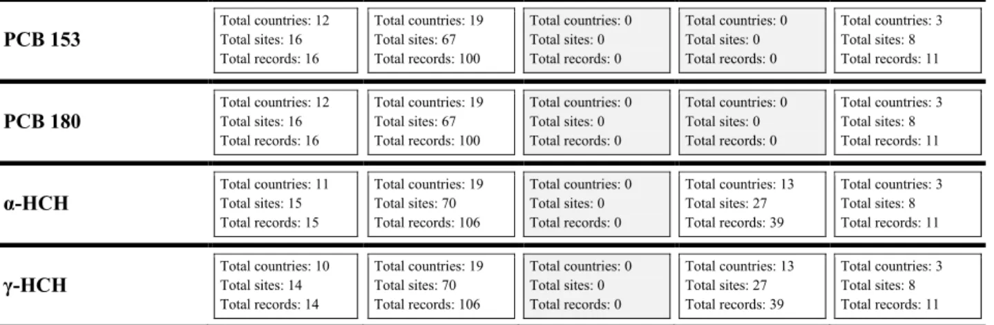
PCB 153 Total countries: 12 Total sites: 16
Total records: 16 Total countries: 19 Total sites: 67 Total records: 100 Total countries: 0 Total sites: 0 Total records: 0 Total countries: 0 Total sites: 0 Total records: 0 Total countries: 3 Total sites: 8 Total records: 11
PCB 180 Total countries: 12 Total sites: 16
Total records: 16 Total countries: 19 Total sites: 67 Total records: 100 Total countries: 0 Total sites: 0 Total records: 0 Total countries: 0 Total sites: 0 Total records: 0 Total countries: 3 Total sites: 8 Total records: 11
α-HCH Total countries: 11 Total sites: 15
Total records: 15 Total countries: 19 Total sites: 70 Total records: 106 Total countries: 0 Total sites: 0 Total records: 0 Total countries: 13 Total sites: 27 Total records: 39 Total countries: 3 Total sites: 8 Total records: 11
γ-HCH Total countries: 10 Total sites: 14
Total records: 14 Total countries: 19 Total sites: 70 Total records: 106 Total countries: 0 Total sites: 0 Total records: 0 Total countries: 13 Total sites: 27 Total records: 39 Total countries: 3 Total sites: 8 Total records: 11
Records: annual POPs concentration values aggregated from primary records by arithmetic mean
Figure 4. Variability analysis of the atmospheric concentrations of POPs in the five UN regions, air monitoring by passive samplers (regional median: boxes; regional geometric mean: circles; regional 5th – 95th percentile ranges: whiskers; global median: grey vertical stripe; global geometric mean:
19
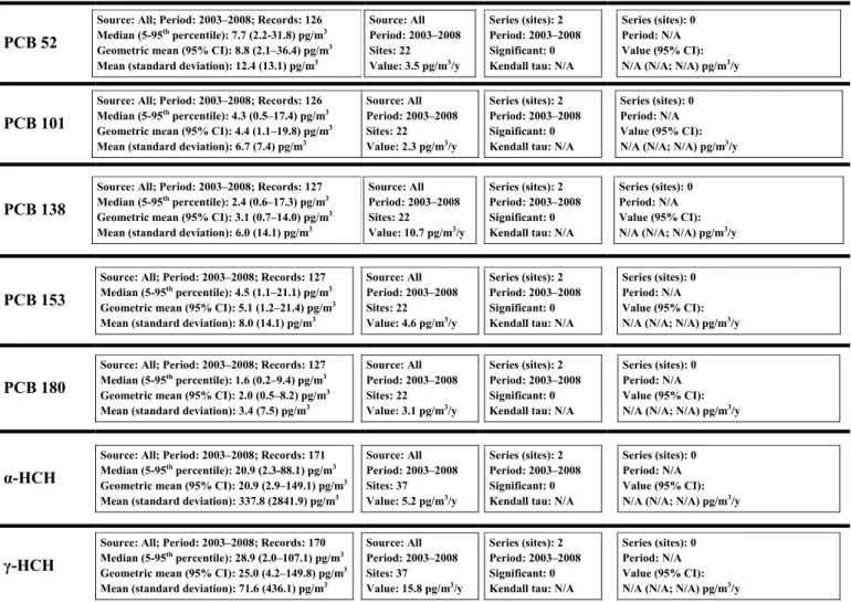
Table 5. Data summary for air monitoring using passive samplers
Compound Baseline concentration alternative Detectable
Historical time trends trend
identification trend quantification
p,p'-DDT
Source: All; Period: 2003–2008; Records: 187 Median (5-95th percentile): 1.8 (0.0–13.2) pg/m3 Geometric mean (95% CI): 2.2 (0.4–12.2) pg/m3 Mean (standard deviation): 9.8 (62.2) pg/m3
Source: All Period: 2003–2008 Sites: 45 Value: 5.3 pg/m3/y Series (sites): 2 Period: 2003–2008 Significant: 0 Kendall tau: N/A
Series (sites): 0 Period: N/A Value (95% CI): N/A (N/A; N/A) pg/m3/y
p,p'-DDE
Source: All; Period: 2003–2008; Records: 197 Median (5-95th percentile): 16.8 (0.0–113.4) pg/m3 Geometric mean (95% CI): 10.3 (1.1–101.1) pg/m3 Mean (standard deviation): 31.7 (65.5) pg/m3
Source: All Period: 2003–2008 Sites: 47 Value: 10.4 pg/m3/y Series (sites): 2 Period: 2003–2008 Significant: 0 Kendall tau: N/A
Series (sites): 0 Period: N/A Value (95% CI): N/A (N/A; N/A) pg/m3/y
HCB
Source: All; Period: 2003–2008; Records: 127 Median (5-95th percentile): 36.0 (7.0–182.3) pg/m3 Geometric mean (95% CI): 32.4 (6.8–153.4) pg/m3 Mean (standard deviation): 48.1 (55.0) pg/m3
Source: All Period: 2003–2008 Sites: 22 Value: 52.0 pg/m3/y Series (sites): 2 Period: 2003–2008 Significant: 2 (2-) Kendall tau: -1.0 Series (sites): 2 Period: 2003–2008 Value (95% CI): -160.1 (-170.2; -150.0) pg/m3/y Σ 6 PCB
Source: All; Period: 1996–2008; Records: 126 Median (5-95th percentile): 30.0 (8.9–159.8) pg/m3 Geometric mean (95% CI): 35.0 (7.4–166.1) pg/m3 Mean (standard deviation): 54.2 (65.1) pg/m3
Source: All Period: 2003–2008 Sites: 22 Value: 22.2 pg/m3/y Series (sites): 2 Period: 2003–2008 Significant: 0 Kendall tau: N/A
Series (sites): 0 Period: N/A Value (95% CI): N/A (N/A; N/A) pg/m3/y
PCB 28
Source: All; Period: 2003–2008; Records: 126 Median (5-95th percentile): 9.0 (2.2–73.6) pg/m3 Geometric mean (95% CI): 10.7 (2.1–53.8) pg/m3 Mean (standard deviation): 19.4 (32.2) pg/m3
Source: All Period: 2003–2008 Sites: 22 Value: 1.2 pg/m3/y Series (sites): 2 Period: 2003–2008 Significant: 0 Kendall tau: N/A
Series (sites): 0 Period: N/A Value (95% CI): N/A (N/A; N/A) pg/m3/y
20
PCB 52
Source: All; Period: 2003–2008; Records: 126 Median (5-95th percentile): 7.7 (2.2-31.8) pg/m3 Geometric mean (95% CI): 8.8 (2.1–36.4) pg/m3 Mean (standard deviation): 12.4 (13.1) pg/m3
Source: All Period: 2003–2008 Sites: 22 Value: 3.5 pg/m3/y Series (sites): 2 Period: 2003–2008 Significant: 0 Kendall tau: N/A
Series (sites): 0 Period: N/A Value (95% CI): N/A (N/A; N/A) pg/m3/y
PCB 101
Source: All; Period: 2003–2008; Records: 126 Median (5-95th percentile): 4.3 (0.5–17.4) pg/m3 Geometric mean (95% CI): 4.4 (1.1–19.8) pg/m3 Mean (standard deviation): 6.7 (7.4) pg/m3
Source: All Period: 2003–2008 Sites: 22 Value: 2.3 pg/m3/y Series (sites): 2 Period: 2003–2008 Significant: 0 Kendall tau: N/A
Series (sites): 0 Period: N/A Value (95% CI): N/A (N/A; N/A) pg/m3/y
PCB 138
Source: All; Period: 2003–2008; Records: 127 Median (5-95th percentile): 2.4 (0.6–17.3) pg/m3 Geometric mean (95% CI): 3.1 (0.7–14.0) pg/m3 Mean (standard deviation): 6.0 (14.1) pg/m3
Source: All Period: 2003–2008 Sites: 22 Value: 10.7 pg/m3/y Series (sites): 2 Period: 2003–2008 Significant: 0 Kendall tau: N/A
Series (sites): 0 Period: N/A Value (95% CI): N/A (N/A; N/A) pg/m3/y
PCB 153
Source: All; Period: 2003–2008; Records: 127 Median (5-95th percentile): 4.5 (1.1–21.1) pg/m3 Geometric mean (95% CI): 5.1 (1.2–21.4) pg/m3 Mean (standard deviation): 8.0 (14.1) pg/m3
Source: All Period: 2003–2008 Sites: 22 Value: 4.6 pg/m3/y Series (sites): 2 Period: 2003–2008 Significant: 0 Kendall tau: N/A
Series (sites): 0 Period: N/A Value (95% CI): N/A (N/A; N/A) pg/m3/y
PCB 180
Source: All; Period: 2003–2008; Records: 127 Median (5-95th percentile): 1.6 (0.2–9.4) pg/m3 Geometric mean (95% CI): 2.0 (0.5–8.2) pg/m3 Mean (standard deviation): 3.4 (7.5) pg/m3
Source: All Period: 2003–2008 Sites: 22 Value: 3.1 pg/m3/y Series (sites): 2 Period: 2003–2008 Significant: 0 Kendall tau: N/A
Series (sites): 0 Period: N/A Value (95% CI): N/A (N/A; N/A) pg/m3/y
α-HCH
Source: All; Period: 2003–2008; Records: 171 Median (5-95th percentile): 20.9 (2.3-88.1) pg/m3 Geometric mean (95% CI): 20.9 (2.9–149.1) pg/m3 Mean (standard deviation): 337.8 (2841.9) pg/m3
Source: All Period: 2003–2008 Sites: 37 Value: 5.2 pg/m3/y Series (sites): 2 Period: 2003–2008 Significant: 0 Kendall tau: N/A
Series (sites): 0 Period: N/A Value (95% CI): N/A (N/A; N/A) pg/m3/y
γ-HCH
Source: All; Period: 2003–2008; Records: 170 Median (5-95th percentile): 28.9 (2.0–107.1) pg/m3 Geometric mean (95% CI): 25.0 (4.2–149.8) pg/m3 Mean (standard deviation): 71.6 (436.1) pg/m3
Source: All Period: 2003–2008 Sites: 37 Value: 15.8 pg/m3/y Series (sites): 2 Period: 2003–2008 Significant: 0 Kendall tau: N/A
Series (sites): 0 Period: N/A Value (95% CI): N/A (N/A; N/A) pg/m3/y
1 Detectable alternative is expressed as the detectable mean annual difference with power = 0.8 and α = 0.05.
The computation is based on the set of sites with available trend data, which are used for the estimation of the variability of differences.
3.5
Results - air monitoring using active sampling
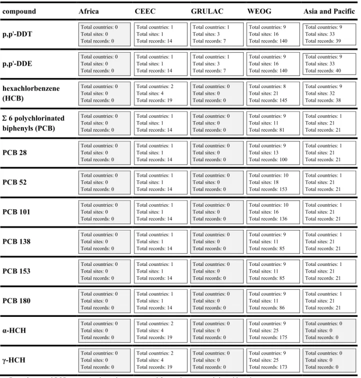
Table 6 contains aggregated entries summarizing data sources for the statistical analysis performed on sites with relevant active concentration data records available. The set consisted of 281 entries from all regions after the six-step validation process described in the introductory section: WEOG (81 records), Asia and Pacific (134 records) and CEEC (66 records). No valid sets were obtained from Africa and GRULAC. The respective cells are shaded if there were no available data entries.
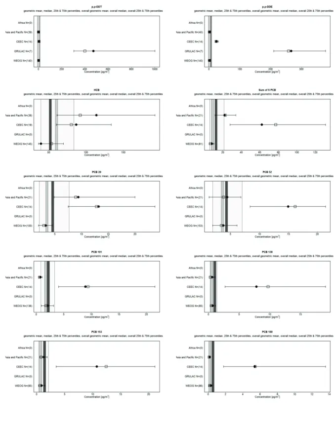
The statistical summary is complemented by the variability/uncertainty analysis provided in Figure 5, consisting of six parts, each part focusing on the individual parameters (compounds) in the analysis. The analysis compares median and geometric mean estimates and their variability among the UN regions. The boxes in the charts indicate medians and the circles geometric means of sets of values for individual regions; whiskers correspond to the 5th – 95th percentile range. The shaded area in the chart corresponds to the 5th – 95th percentile range of the entire set of sites for all regions. The grey vertical stripe corresponds to the global median estimate and black vertical stripe corresponds to the global geometric mean of this set.
Table 7 displays results of the statistical analysis of the validated atmospheric POPs concentrations obtained by active sampling. Both baseline concentrations and historical time trends are estimated.
21
Table 6. Data sources for air monitoring using active sampling (if data entries from no site are available, the cell is shaded)
compound Africa CEEC GRULAC WEOG Asia and Pacific
p,p'-DDT Total countries: 0 Total sites: 0
Total records: 0 Total countries: 1 Total sites: 1 Total records: 14 Total countries: 1 Total sites: 3 Total records: 7 Total countries: 9 Total sites: 16 Total records: 140 Total countries: 9 Total sites: 33 Total records: 39
p,p'-DDE Total countries: 0 Total sites: 0
Total records: 0 Total countries: 1 Total sites: 1 Total records: 14 Total countries: 1 Total sites: 3 Total records: 7 Total countries: 9 Total sites: 16 Total records: 140 Total countries: 9 Total sites: 33 Total records: 40 hexachlorbenzene (HCB) Total countries: 0 Total sites: 0 Total records: 0 Total countries: 2 Total sites: 4 Total records: 19 Total countries: 0 Total sites: 0 Total records: 0 Total countries: 8 Total sites: 21 Total records: 145 Total countries: 9 Total sites: 32 Total records: 38 Σ 6 polychlorinated biphenyls (PCB) Total countries: 0 Total sites: 0 Total records: 0 Total countries: 1 Total sites: 1 Total records: 14 Total countries: 0 Total sites: 0 Total records: 0 Total countries: 9 Total sites: 11 Total records: 81 Total countries: 1 Total sites: 21 Total records: 21
PCB 28 Total countries: 0 Total sites: 0
Total records: 0 Total countries: 1 Total sites: 1 Total records: 14 Total countries: 0 Total sites: 0 Total records: 0 Total countries: 9 Total sites: 13 Total records: 100 Total countries: 1 Total sites: 21 Total records: 21
PCB 52 Total countries: 0 Total sites: 0
Total records: 0 Total countries: 1 Total sites: 1 Total records: 14 Total countries: 0 Total sites: 0 Total records: 0 Total countries: 10 Total sites: 18 Total records: 153 Total countries: 1 Total sites: 21 Total records: 21
PCB 101 Total countries: 0 Total sites: 0
Total records: 0 Total countries: 1 Total sites: 1 Total records: 14 Total countries: 0 Total sites: 0 Total records: 0 Total countries: 10 Total sites: 16 Total records: 136 Total countries: 1 Total sites: 21 Total records: 21
PCB 138 Total countries: 0 Total sites: 0
Total records: 0 Total countries: 1 Total sites: 1 Total records: 14 Total countries: 0 Total sites: 0 Total records: 0 Total countries: 9 Total sites: 11 Total records: 85 Total countries: 1 Total sites: 21 Total records: 21
PCB 153 Total countries: 0 Total sites: 0
Total records: 0 Total countries: 1 Total sites: 1 Total records: 14 Total countries: 0 Total sites: 0 Total records: 0 Total countries: 9 Total sites: 11 Total records: 85 Total countries: 1 Total sites: 21 Total records: 21
PCB 180 Total countries: 0 Total sites: 0
Total records: 0 Total countries: 1 Total sites: 1 Total records: 14 Total countries: 0 Total sites: 0 Total records: 0 Total countries: 9 Total sites: 11 Total records: 86 Total countries: 1 Total sites: 21 Total records: 21
α-HCH Total countries: 0 Total sites: 0
Total records: 0 Total countries: 2 Total sites: 4 Total records: 19 Total countries: 0 Total sites: 0 Total records: 0 Total countries: 9 Total sites: 25 Total records: 175 Total countries: 0 Total sites: 0 Total records: 0
γ-HCH Total countries: 0 Total sites: 0
Total records: 0 Total countries: 2 Total sites: 4 Total records: 19 Total countries: 0 Total sites: 0 Total records: 0 Total countries: 9 Total sites: 25 Total records: 173 Total countries: 0 Total sites: 0 Total records: 0
22
Figure 5. Variability analysis of atmospheric concentrations of POPs in the five UN regions, air monitoring using active sampling (regional median: boxes; regional geometric mean: circles; regional 5th – 95th percentile ranges: whiskers; global median: grey vertical stripe; global geometric
23
Table 7. Data summary for air monitoring using active sampling
Compound
Overall concentration alternativeDetectable 1
Historical time trends trend
identification quantification trend
p,p'-DDT
Source: All; Period: 1996–2009; Records: 200 Median (5-95th percentile): 0.8 (0.0–25.7) pg/m3 Geometric mean (95% CI): 1.8 (0.2–12.5) pg/m3 Mean (standard deviation): 26.2 (161.1) pg/m3
Source: All Period: 1990–2009 Sites: 23 Value: 188.6 pg/m3/y Series (sites): 12 Period: 1990–2009 Significant: 4 (4-) Kendall tau: -0.6 Series (sites): 4 Period: 1992–2008 Value (95% CI): -0.9 (-1.6; -0.2) pg/m3/y p,p'-DDE
Source: All; Period: 1996–2009; Records: 201 Median (5-95th percentile): 1.8 (0.2–43.6) pg/m3 Geometric mean (95% CI): 3.5 (0.5–24.8) pg/m3 Mean (standard deviation): 16.6 (60.9) pg/m3
Source: All Period: 1990–2009 Sites: 24 Value: 20.6 pg/m3/y Series (sites): 13 Period: 1990–2009 Significant: 4 (4-) Kendall tau: -0.6 Series (sites): 4 Period: 1992–2009 Value (95% CI): -5.3 (-15.2; 4.6) pg/m3/y hexachlorbenzene (HCB)
Source: All; Period: 1993–2009; Records: 202 Median (5-95th percentile): 60.5 (5.7–202.5) pg/m3 Geometric mean (95% CI): 52.2 (9.2–296.4) pg/m3 Mean (standard deviation): 89.7 (176.1) pg/m3
Source: All Period: 1990–2009 Sites: 25 Value: 31.1 pg/m3/y Series (sites): 13 Period: 1990–2009 Significant: 4 (4-) Kendall tau: -0.4 Series (sites): 4 Period: 1991–2008 Value (95% CI): -19.8 (-57.2; 17.5) pg/m3/y Σ 6 polychlorinated biphenyls (PCB)
Source: All; Period: 1996–2008; Records: 116 Median (5-95th percentile): 8.8 (4.5–100.8) pg/m3 Geometric mean (95% CI): 12.7 (2.6–61.7) pg/m3 Mean (standard deviation): 22.4 (34.2) pg/m3
Source: All Period: 1993–2009 Sites: 12 Value: 27.5 Series (sites): 9 Period: 1993–2009 Significant: 5 (4-; 1+) Kendall tau: 0.5 Series (sites): 5 Period: 1995–2009 Value (95% CI): -28.1 (-110.2;54.0) pg/m3/y PCB 28
Source: All; Period: 1996–2009; Records: 135 Median (5-95th percentile): 3.5 (1.3–24.2) pg/m3 Geometric mean (95% CI): 4.6 (1.1–19.7) pg/m3 Mean (standard deviation): 7.2 (10.8) pg/m3
Source: All Period: 1992–2009 Sites: 14 Value: 4.9 Series (sites): 11 Period: 1992–2009 Significant: 3 (3-) Kendall tau: -0.8 Series (sites): 3 Period: 1994–2009 Value (95% CI): -8.3 (-15.0; -1.6) pg/m3/y PCB 52
Source: All; Period: 1996–2009; Records: 188 Median (5-95th percentile): 3.6 (1.0–20.4) pg/m3 Geometric mean (95% CI): 4.3 (1.0–18.2) pg/m3 Mean (standard deviation): 6.5 (8.0) pg/m3
Source: All Period: 1990–2009 Sites: 18 Value: 5.2 Series (sites): 15 Period: 1990–2009 Significant: 7 (5-; 2+) Kendall tau: -0.2 Series (sites): 7 Period: 1991–2009 Value (95% CI): -3.5 (-17.3; 10.3) pg/m3/y PCB 101
Source: All; Period: 1996–2009; Records: 171 Median (5-95th percentile): 1.7 (0.4–11.5) pg/m3 Geometric mean (95% CI): 2.2 (0.5–8.8) pg/m3 Mean (standard deviation): 3.4 (5.1) pg/m3
Source: All Period: 1990–2009 Sites: 16 Value: 2.9 Series (sites): 13 Period: 1990–2009 Significant: 7 (5-; 2+) Kendall tau: -0.2 Series (sites): 7 Period: 1991–2009 Value (95% CI): -1.6 (-6.6; 3.4) pg/m3/y PCB 138
Source: All; Period: 1996–2009; Records: 120 Median (5-95th percentile): 0.5 (0.1–10.0) pg/m3 Geometric mean (95% CI): 1.0 (0.2–4.3) pg/m3 Mean (standard deviation): 2.2 (5.1) pg/m3
Source: All Period: 1993–2009 Sites: 12 Value: 6.0 Series (sites): 9 Period: 1993–2009 Significant: 4 (4-) Kendall tau: -0.6 Series (sites): 4 Period: 1993–2009 Value (95% CI): -6.9 (-27.7; 13.9) pg/m3/y PCB 153
Source: All; Period: 1996–2009; Records: 120 Median (5-95th percentile): 0.7 (0.2–12.9) pg/m3 Geometric mean (95% CI): 1.4 (0.3–6.2) pg/m3 Mean (standard deviation): 3.1 (7.3) pg/m3
Source: All Period: 1993–2009 Sites: 12 Value: 8.2 Series (sites): 9 Period: 1993–2009 Significant: 4 (4-) Kendall tau: -0.6 Series (sites): 4 Period: 1994–2009 Value (95% CI): -9.4 (-37.0; 18.2) pg/m3/y
24
PCB 180
Source: All; Period: 1996–2009; Records: 121 Median (5-95th percentile): 0.2 (0.0–5.8) pg/m3 Geometric mean (95% CI): 0.5 (0.1–2.1) pg/m3 Mean (standard deviation): 1.3 (4.2) pg/m3
Source: All Period: 1993–2009 Sites: 12 Value: 6.8 Series (sites): 9 Period: 1993–2009 Significant: 5 (5-) Kendall tau: -0.6 Series (sites): 5 Period: 1993–2009 Value (95% CI): -6.0 (-28.4; 16.5) pg/m3/y α-HCH
Source: All; Period: 1993–2009; Records: 194 Median (5-95th percentile): 18.1 (1.2–87.8) pg/m3 Geometric mean (95% CI): 17.9 (3.2–99.8) pg/m3 Mean (standard deviation): 29.7 (34.9) pg/m3
Source: All Period: 1990–2009 Sites: 24 Value: 25.0 pg/m3/y Series (sites): 15 Period: 1990–2009 Significant: 12 (12-) Kendall tau: -0.9 Series (sites): 12 Period: 1990–2008 Value (95% CI): -49.6 (-129.4; 30.3) pg/m3/y γ-HCH
Source: All; Period: 1993–2009; Records: 192 Median (5-95th percentile): 9.9 (0.6–50.8) pg/m3 Geometric mean (95% CI): 9.5 (1.9–46.6) pg/m3 Mean (standard deviation): 14.9 (17.8) pg/m3
Source: All Period: 1990–2009 Sites: 23 Value: 13.4 pg/m3/y Series (sites): 15 Period: 1990–2009 Significant: 10 (10-) Kendall tau: -0.7 Series (sites): 10 Period: 1990–2008 Value (95% CI): -17.3 (-51.5; 17.0) pg/m3/y
1 The detectable alternative is expressed as the detectable mean annual difference with power = 0.8 and α = 0.05.
The computation is based on the set of sites with available trend data, which are used for the estimation of the variability of time-related differences.
25
4
Reporting of GMP data collected in the period 1998-2008 and its
extension
Interactive reporting tools prepared for the GMP 2 campaign are based on the on-line visualization created for GMP 1 (see www.pops-gmp.org/visualization) to ensure consistency of reported content; functionality of these tools for the GMP 2 purposes is broadened for time series analysis and
additional map functions. All tools share standardized data selection and customization of analysis settings.
4.1
World map – monitoring overview
An animated map shows the geographical coverage of data with predefined filters for displaying available datasets: matrix, compound and year. For the latter, the user has the option to select a single point in time or a time interval. The user gets data coverage for a selected matrix and a point or interval in time or data coverage for a particular point/interval in time, matrix and compound as the output.
26
Figure 7. Coverage of countries by monitoring
4.2
Available data – parameters
A chart shows sampling frequency for each compound in a particular year (user-defined). Compounds are listed on x-axis, countries on y-axis. The predefined filters include: matrix, sampling method (for air), type of measurement site (for air – urban, rural, remote etc.), UN region, compound and year. Detailed data are displayed by clicking on a chart cell. Multiple selections are enabled in the predefined filters.
Figure 8. Available data – parameters
4.3
Available data – years
Chart shows the sampling frequency in a user-defined time period. Years are listed on x-axis,
countries on y-axis. Predefined filters for the selection include: matrix, sampling method (for air), type of measurement site (for air – urban, rural, remote etc.), UN region, compound and time period (three
27
years at a minimum). Detailed data are displayed by clicking on a chart cell. Multiple selections are enabled in the predefined filters.
Figure 9. Available data – years
4.4
Reported values – summary statistics
Chart shows a summary statistics for each reported value (mean, median, min, max). Concentration values are displayed in the form of box-and-whisker plots with mean/median value, minimum and maximum. Concentrations are listed on x-axis, reported sites/countries on y-axis. The predefined filters include: matrix, sampling method (for air), type of measurement site (for air – urban, rural, remote etc.), UN region, compound and year.
4.5
Reported values – advanced interactive map visualization
The output is a map with visualization at each site corresponding to the measured POPs concentrations (the user can select prioritized statistics, mean, median, etc.). Filters for the analysis include: matrix, sampling method (for air), type of measurement site (for air – urban, rural, remote etc.), compound, year, UN region. Multiple selections are enabled for the list of compounds / years. The map allows interactive panning and zooming.
4.6
Time series analysis
The report offers screening examination of the trends in data as well as exact statistical evaluation of the trend significance via standard tests (according to the GMP guidance document, Chapter 3: “Statistical Considerations and the Technical Note to Chapter 3”). Filters for the analysis include: matrix, compound and measurement site. The option to adjust the analysis settings, e.g., selection of the method for trend evaluation, is available.
28
Figure 10. Reported values – summary statistics
29
30
5
Documentation of new GIS module proposed for GMP DWH
A GIS server extends functions of the GMP Data warehouse by providing support for spatial data visualizations, map distribution and for performing spatial analysis in real-time. The GIS server also allows linking additional information to stored data, all based on spatial references.
GIS Server is an important module of common ICT (information and communication technologies) infrastructure which provides technological background to all GMP DWH tools and services. GIS server is connected to the GMP DWH and provides data, together with application server and R server, in a form suitable for presentation, visualization and exports.
31
GIS module of GMP DWH enables work with spatial data. GIS server custom software components will be developed to enable visualization of spatial data, their analysis, extraction of the hidden information and performing advanced spatially based queries, processing and transformations.
Table 8. Specification of new GIS module functions in the GMP DWS GIS Module for GMP DWH
Software Component Technology background Benefits
GIS server integration GIS server is based on the
ESRI´s ArcGIS Server integration. ArcGIS server represents hi-end technology in the area of GIS and provides a broad range of additional features for data integration and interoperability.
ArcGIS Server enables to publish static map
compositions, generate dynamic map layers based on data from various sources, process calculations over spatial features based on individual user inputs. In general, GIS server provides a platform for publishing and sharing spatially based information.
Dynamic map services Integration of ArcGIS Server
with the database and data services of GMP DWH.
Interconnection of ArcGIS Server with GMP data
warehouse enables creation of specialized map layers
dynamically generated from the current data warehouse content. This enables, e.g., development of map visualizations of a selected pollutant in a given geographic area and in a specific time range.
GMP Spatial Web Engine Web technologies, software
libraries for communication with ArcGIS Server (ArcGIS API for JavaScript / Flex) and specialized software
frameworks and technologies focused on spatial and data visualizations.
GMP Spatial Web Engine is a specialized software product derived from the GIS module. GMP Spatial Web Engine is based on the common web technologies and is accessible via the Internet. The engine is connected to GIS server and other software components. GMP Spatial Web Engine is a basic platform on which other software components are being developed in a form of plugins (software extensions).
Map Browser Plugin
for GMP Spatial Web Engine GMP Spatial web engine, web technologies, software libraries for communication with ArcGIS Server.
Map Browser Plugin allows displaying map services
published upon GMP DWH in a common internet browser. GMP Spatial Web Engine
- interoperability Interoperability of whole GIS Module is ensured by support of standardized data formats designed by OGC (Open Geospatial Consortium).
Feature of inserting custom map layers enables users to combine prepared map layers with custom map services published on any server accessible via the
32
Internet. GMP Spatial Web Engine
- import feature GMP Spatial Web Engine, data formats able to store tabular data.
GMP Spatial Web Engine enables inserting spatial data directly from the user's computer and display them together with prepared map layers in one composition. Time-lapse spatial
visualizations Time-lapse spatial visualizations are based on the
so called time aware feature layer of ArcGIS.
Time aware feature layers will be used to visualize temporally changing spatial data in appropriate cases.
Geoprocessing Based on geo-processing
capabilities of ArcGIS Server. In general, geo-processing services enable to create calculations over spatial data. Results can be used in map compositions accessible via Map Browser of GIS Module. Quality print capabilities and
export to PDF GMP Spatial web engine, web technologies, software libraries for communication with ArcGIS Server.
GIS Module is equipped with quality print and export engine; thus, the whole GIS Module can be used as a tool for creating reports.