Numerical Solutions of First Order Initial-Value
Problem with Singularities and Stiffness
Properties by a Rational Scheme
A.N. Fairuz1, Z.A. Majid1,2∗ and Z.B. Ibrahim2
1Institute for Mathematical Research, Universiti Putra Malaysia,
43400 UPM Serdang, Selangor, Malaysia
2Department of Mathematics, Faculty of Science, Universiti Putra Malaysia,
43400 UPM Serdang, Selangor, Malaysia
In this paper, a scheme for solving first order singular and stiff differential equations is proposed. The studied approaches, namely Modified Rational Method (MRM), are developed based on a rational function mentioned by an existing study and possess second and third order of accura cy. Some modifications is implemented in the derivation technique, where closest points of approximation are considered in the formula of the methods. The proposed methods are both A -stable and suitable in solving problems with stiffness properties. The methods are not self-starting, thus the application of a suitable method to calculate the starting value is required in implementing these formulas. The results computed by the methods are found to be comparable to the existing methods.
Keywords: explicit rational method; singular initial-value problem; stiff DE
I. INTRODUCTION
Studies on numerical approaches that are developed for solving initial value problems (IVPs) of the form
𝑦′= 𝑓(𝑥, 𝑦), 𝑦(𝑎) = 𝑦
0, 𝑥 ∈ [𝑎, 𝑏],
where 𝑎 and 𝑏 are the initial and the end points of the interval of 𝑥 respectively, usually came from the class of linear methods, such as Linear Multistep Methods and Runge-Kutta Methods. Some methods are specially formulated for specific problems; for instance, Backward Differentiation Formula (BDF) for solving stiff problems and Rational Method for solving problems with singularity.
The suitability of numerical approaches that are based on rational function, or better known as rational method in solving many types of problems has intrigued many researchers to study more on this topic. Some literature rational methods are such as (Lambert & Shaw, 1965; Niekerk, 1987; Niekerk, 1988; Ikhile, 2001) for one-step schemes, while (Luke et al., 1975; Fatunla, 1982; Fatunla, 1986; Abelman &
Eyre, 1990; Okosun & Ademiluyi, 2007a; 2007b) for multistep schemes. Some studies on this topic focus on developing A-stable rational schemes so that the methods are suitable in solving stiff problems, for instance; (Ramos, 2007; Ramos et al., 2015; Ramos et al., 2017; Teh et al., 2011).
One of the recent studies on rational multistep methods are done by (Teh & Yaacob, 2013), namely RMM3 which have the form of
𝑦𝑛+2= 𝑦𝑛+
2ℎ(𝑦𝑛′)2
𝑦𝑛′ − ℎ𝑦𝑛′′
. (1)
From the formula, it is obvious that the distance between the approximation points is two steplengths, or 2ℎ. Motivated by the study, we aim to develop a class of rational methods that will lessen the gap of the selected points of approximation. In order to develop such methods, we implement some modifications in the derivation technique of the proposed methods.
ensured to facilitate the comparisons between the methods studied and some existing methods. The development, order, stability and implementations of the methods will be discussed in this paper. The presented methods in this article are examined on different types of problem; singular and stiff IVPs and the results are compared to the existing methods.
II. FRAMEWORK OF
MODIFIED RATIONAL METHODS (MRM)
By referring to (Teh and Yaacob, 2013), we suggest the
approximation for y(xn+2) denoted by yn+2 and is given by;
𝑦𝑛+2= 𝐵 + ℎ [
𝐴ℎ ∑𝐾𝑗=1𝑐𝑗ℎ𝑗
], (2)
where 𝐴 is real constant, while 𝐵 and 𝑐𝑗, 𝑗 = 1,2, … , 𝐾 are
parameters that may contain approximations of 𝑦(𝑥𝑛+1) and
higher derivatives of 𝑦(𝑥𝑛+1).
With the formula above, we associate the linear difference
operator;
𝐿[𝑦(𝑥); ℎ]𝑀𝑅𝑀= [𝑦(𝑥𝑛+2) − 𝐵] × [∑ 𝑐𝑗ℎ𝑗 𝐾
𝑗=1
] − 𝐴ℎ
= [𝑦(𝑥𝑛+1+ ℎ) − 𝐵] × [∑ 𝑐𝑗ℎ𝑗 𝐾
𝑗=1
]
− 𝐴ℎ,
(3)
where 𝑦(𝑥𝑛+1+ ℎ) is chosen to represent 𝑦(𝑥𝑛+2) in order to
lessen the gap between the approximated point and the point
which is considered for the approximation process by the
formula of the method. Meanwhile, 𝑦(𝑥) is arbitrary and
continuously differentiable on 𝑥 ∈ [𝑎, 𝑏]. Next is to expand
𝑦(𝑥𝑛+1+ ℎ) as Taylor series around 𝑥𝑛+1and collecting terms in
the difference operator in (3), and we will obtain an expression
that can be generally written as;
𝐿[𝑦(𝑥); ℎ]𝑀𝑅𝑀= 𝐶0ℎ0+ 𝐶1ℎ1+ ⋯ + 𝐶𝐾ℎ𝐾
+ 𝐶𝐾+1ℎ𝐾+1+ ⋯.
(4
)
Note that 𝐶𝑖, 𝑖 = 0,1, … , 𝐾, 𝐾 + 1 in expression (4) contain the
parameters that are to be determined throughout the
derivation process. The order and the parameters can be
determined by referring to the definition:
Definition 1. The difference operator in equation (3) and the associated rational method (2) are said to be of order
𝑝 = 𝐾 + 1 if, in expression (4), 𝐶0= 𝐶1= ⋯ = 𝐶𝐾= 𝐶𝐾+1=
0, 𝐶𝐾+2≠ 0.
Meanwhile, The local truncation errors of MRM are
determined based on the definition below;
Definition 2. The local truncation error at 𝑥𝑛+2 of
equation (2) is defined to be the expression 𝐿[𝑦(𝑥); ℎ]𝑀𝑅𝑀
given by equation (3), when 𝑦(𝑥𝑛+1) is the theoretical
solution of the initial value problem at a point 𝑥𝑛+1. The
local truncation error of equation (2) is then
𝐿[𝑦(𝑥); ℎ]𝑀𝑅𝑀 = 𝐶𝐾+2ℎ𝐾+2+ 𝑂(ℎ𝐾+3) . (5)
A. Second Order Modified Rational Method (MRM(2))
In order to have the second order of MRM, we consider 𝐾 =
1 in (2) so we will have the rational function in the form of;
𝑦𝑛+2= 𝐵 +
𝐴ℎ
1 + 𝑐1ℎ, where 1 + 𝑐1ℎ ≠ 0
(6)
and its associated linear difference operator as;
𝐿[𝑦(𝑥); ℎ]𝑀𝑅𝑀(2)= [𝑦(𝑥𝑛+1+ ℎ) − 𝐵]
× (1 + 𝑐1ℎ) − 𝐴ℎ
(7
)
Next, expanding 𝑦(𝑥𝑛+1+ ℎ) as Taylor series around 𝑥𝑛+1
will give the expression;
𝐿[𝑦(𝑥); ℎ]𝑀𝑅𝑀(2)= −𝐵 + 𝑦(𝑥𝑛+1)
+ ℎ[−𝐴 − 𝐵𝑐1+ 𝑐1𝑦(𝑥𝑛+1) + 𝑦′(𝑥𝑛+1)]
+ ℎ2[𝑐
1𝑦′(𝑥𝑛+1) +
1 2𝑦
′′(𝑥 𝑛+1)]
+ ℎ3[1
2𝑐1𝑦
′′(𝑥 𝑛+1) +
1 6𝑦
′′′(𝑥
𝑛+1)] + 𝑂(ℎ4)
(8)
From (8), we obtain;
𝐶0= −𝐵 + 𝑦(𝑥𝑛+1)
𝐶1= −𝐴 − 𝐵𝑐1+ 𝑐1𝑦(𝑥𝑛+1) + 𝑦′(𝑥𝑛+1)
𝐶2= 𝑐1𝑦′(𝑥𝑛+1) +
1 2𝑦
′′(𝑥 𝑛+1)
𝐶3=
1 2𝑐1𝑦
′′(𝑥 𝑛+1) +
1 6𝑦
′′′(𝑥 𝑛+1)
Since 𝐾 = 1 and according to Definition 1, 𝐶0= 𝐶1= 𝐶2= 0
and 𝐶3≠ 0; and we take 𝑦𝑛+1 as the approximation of the
theoretical solution 𝑦(𝑥𝑛+1), thus the parameters in (6) are
determined and can be written as;
𝐴 = 𝑦𝑛+1 ′ ,
𝐵 = 𝑦𝑛+1 ,
𝑐1= −
𝑦𝑛+1′′
2𝑦𝑛+1′
,
(10
)
where by the localizing assumption, 𝑦𝑛+1= 𝑦(𝑥𝑛+1) and
𝑦𝑛+1𝑚 = 𝑦𝑚(𝑥𝑛+1), 𝑚 = 1,2.
By substituting the obtained parameters in (10) in 𝐶3, we have;
𝐶3= −
(𝑦𝑛+1′′ )2
4𝑦𝑛+1′ +
𝑦𝑛+1′′′
6 . (11)
Based on equation (6) and (10), we formulate MRM(2) and it
can be written as;
𝑦𝑛+2= 𝑦𝑛+1+
2ℎ(𝑦𝑛+1′ )2
2𝑦𝑛+1′ − ℎ𝑦𝑛+1′′
. (12)
As we refer to Definition 2 and (11), we obtain the local
truncation error for MRM(2):
𝐿𝑇𝐸𝑀𝑅𝑀(2)= ℎ3[−
(𝑦𝑛+1′′ )2
4𝑦𝑛+1′
+𝑦𝑛+1
′′′
6 ]
+ 𝑂(ℎ4),
(13)
where by the localizing assumption, 𝑦𝑛+1𝑚 = 𝑦𝑚(𝑥𝑛+1), 𝑚 =
1,2,3.
B. Third Order Modified Rational Method (MRM(3))
To derive a third order MRM, we need to consider 𝐾 = 2 in (2)
so the rational approximation associated to this method is
𝑦𝑛+2= 𝐵 +
𝐴ℎ 1 + 𝑐1ℎ + 𝑐2ℎ2
,
where 1 + 𝑐1ℎ + 𝑐2ℎ2≠ 0
(14)
and the associated linear difference operator is given as
𝐿[𝑦(𝑥); ℎ]𝑀𝑅𝑀(2)= [𝑦(𝑥𝑛+1+ ℎ) − 𝐵]
× (1 + 𝑐1ℎ + 𝑐2ℎ2) − 𝐴ℎ
(15)
Next, we expand 𝑦(𝑥𝑛+1+ ℎ) as Taylor series to have the
expression;
𝐿[𝑦(𝑥); ℎ]𝑀𝑅𝑀(2)= −𝐵 + 𝑦(𝑥𝑛+1)
+ ℎ[−𝐴 − 𝐵𝑐1+ 𝑐1𝑦(𝑥𝑛+1) + 𝑦′(𝑥𝑛+1)]
+ ℎ2[−𝐵𝑐
2+ 𝑐2𝑦(𝑥𝑛+1) + 𝑐1𝑦′(𝑥𝑛+1)
+1
2𝑦′′(𝑥𝑛+1)]
+ ℎ3[𝑐
2𝑦′(𝑥𝑛+1) +
1 2𝑐1𝑦
′′(𝑥 𝑛+1) +
1 6𝑦
′′′(𝑥 𝑛+1)]
+ ℎ4[1
2𝑐2𝑦
′′(𝑥 𝑛+1) +
1 6𝑐1𝑦
′′′(𝑥 𝑛+1) +
1 24𝑦𝑛+1
(4)
]
+ 𝑂(ℎ5)
(16)
From (16); we obtain;
𝐶0= −𝐵 + 𝑦(𝑥𝑛+1)
𝐶1= −𝐴 − 𝐵𝑐1+ 𝑐1𝑦(𝑥𝑛+1) + 𝑦′(𝑥𝑛+1)
𝐶2= −𝐵𝑐2+ 𝑐2𝑦(𝑥𝑛+1) + 𝑐1𝑦′(𝑥𝑛+1) +
1 2(𝑥𝑛+1)
𝐶3= 𝑐2𝑦′(𝑥𝑛+1) +
1 2𝑐1𝑦
′′(𝑥 𝑛+1) +
1 6𝑦
′′′(𝑥 𝑛+1)
𝐶4=
1 2𝑐2𝑦
′′(𝑥 𝑛+1) +
1 6𝑐1𝑦
′′′(𝑥 𝑛+1) +
1 24𝑦𝑛+1
(4)
(17)
Since 𝐾 = 2 and by following Definition 1, we have 𝐶0=
𝐶1= 𝐶2= 𝐶3= 0 and 𝐶4≠ 0 , taking 𝑦𝑛+1 as the
approximation of the theoretical solution 𝑦(𝑥𝑛+1), thus the
parameters in (14) are determined as;
𝐴 = 𝑦𝑛+1 ′ ,
𝐵 = 𝑦𝑛+1 ,
𝑐1= −
𝑦𝑛+1′′
2𝑦𝑛+1′ ,
𝑐2=
3(𝑦𝑛+1′′ )2− 2𝑦𝑛+1′ 𝑦𝑛+1′′′
12(𝑦𝑛+1′ )2 ,
(18
)
where by the localizing assumption, 𝑦𝑛+1= 𝑦(𝑥𝑛+1) and
𝑦𝑛+1𝑚 = 𝑦𝑚(𝑥𝑛+1), 𝑚 = 1,2,3.
By substituting the obtained parameters in (18) in 𝐶4, we
𝐶4=
(𝑦𝑛+1′′ )3
8(𝑦𝑛+1′ )2
−𝑦𝑛+1
′′ 𝑦 𝑛+1′′′
6𝑦𝑛+1′
+ 1 24𝑦𝑛+1
(4)
. (19)
Based on equation (14) and (18) we formulate MRM(3) and it
can be written as;
𝑦𝑛+2= 𝑦𝑛+1+
12ℎ(𝑦𝑛+1′ )3
[ 12(𝑦𝑛+1
′ )2− 6ℎ𝑦 𝑛+1′ 𝑦𝑛+1′′
+3ℎ2(𝑦
𝑛+1′′ )2− 2ℎ2𝑦𝑛+1′ 𝑦𝑛+1′′′
]
. (20)
Referring to Definition 2 and (20), we obtain the local
truncation error for MRM(3).
𝐿𝑇𝐸𝑀𝑅𝑀(3)= ℎ4[
(𝑦𝑛+1′′ )3
8(𝑦𝑛+1′ )2−
𝑦𝑛+1′′ 𝑦𝑛+1′′′
6𝑦𝑛+1′
+ 1 24𝑦𝑛+1
(4)
] + 𝑂(ℎ4),
(21)
where by the localizing assumption,
𝑦𝑛+1𝑚 = 𝑦𝑚(𝑥𝑛+1), 𝑚 = 1,2,3,4.
III. STABILITY REGIONS OF
MRM
The stability of the proposed rational methods can be analysed
by applying it the Dahlquist's test equation, 𝑦′= 𝜆𝑦, 𝑅𝑒(𝜆) <
0.
The A-stability of the methods can be identified according to
the definition below;
Definition 3. A numerical method is said to be A-stable if its region of absolute stability contains the whole left-hand
half-plane Re ℎ𝜆 < 0.
A. Stability of MRM(2)
To find the stability region for MRM(2) in (12), the formula of
the method is applied to the test equation, and it yields the
difference equation;
𝑦𝑛+2= 𝑦𝑛+1+ [
2 + 𝜆ℎ
2 − 𝜆ℎ] . (22)
Taking 𝑧 = ℎ𝜆, 𝑦𝑛+2= 𝜉2, and 𝑦𝑛+1= 𝜉1, simplifying it and
the stability function and the root, 𝜉 can be obtained as;
𝑅(𝑧)𝑀𝑅𝑀(2)= 𝜉 = [
2 + 𝑧
2 − 𝑧] . (23)
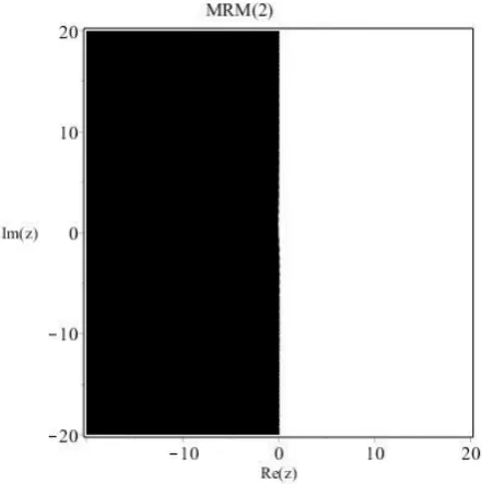
Taking 𝑧 = 𝑥 + 𝑖𝑦 into (23), we have plotted the absolute
stability region of MRM(2) as in Figure 1, with the condition
|𝑅(𝑧)𝑀𝑅𝑀(2)| ≤ 1 is satisfied.
Since the plotted stability region of MRM(2) (refer to
Figure 1) is unbounded and contains the whole left-hand
half-plane, thus it can be concluded that the second-order
method is A-stable.
Figure 1. Absolute stability region of MRM(2)
B. Stability of MRM(3)
As MRM(3) in (20) is applied to the test equation, it gives
the difference equation;
𝑦𝑛+2= 𝑦𝑛+1+ [
12 + 6𝜆ℎ + 𝜆2ℎ2
12 − 6𝜆ℎ + 𝜆2ℎ2] . (24)
Taking 𝑧 = ℎ𝜆, 𝑦𝑛+2= 𝜉2, and 𝑦𝑛+1= 𝜉1, simplifying it
and the stability function and the root, 𝜉 can be obtained as;
𝑅(𝑧)𝑀𝑅𝑀(3)= 𝜉 = [
12 + 6𝑧 + 𝑧2
12 − 6𝑧 + 𝑧2] . (25)
Taking 𝑧 = 𝑥 + 𝑖𝑦 into (25), we have plotted the absolute
stability region of MRM(3) with the condition
similar to the stability region of MRM(2), thus this method can
also be concluded as A-stable.
IV. IMPLEMENTATION
The first step to implement the rational scheme developed in
this study is to choose a suitable method to calculate the
starting values as both methods are not self-starting. In this
article, we apply the rational method of order four that is
proposed by (Lambert, 1973) to compute the starting values.
The formula of the method is given by;
𝑦𝑛+1= 𝑦𝑛+ ℎ𝑦𝑛′+
ℎ2
2 𝑦𝑛
′′+ℎ3
6 𝑦𝑛
′′′
+ℎ
4
6 [ 𝑦𝑛′′′𝑦𝑛
(4)
4𝑦𝑛′′′− ℎ𝑦𝑛 (4)]
(26)
Based on the formulation of the proposed rational methods;
it is necessary to determine higher derivatives of the problem
in order to compute the numerical solution. To obtain the
higher derivatives of the IVP, differentiation of the equation of
the problem is required;
𝑦(𝑘+1)(𝑥)|
𝑥=𝑥𝑛+1=
𝑑𝑓𝑘(𝑥, 𝑦(𝑥))
𝑑𝑥𝑘 |
𝑥=𝑥𝑛+1 ≈ 𝑦𝑛+1
(𝑘+1)
. (27)
In this article, we compare the numerical results by MRM
with several existing methods that have been introduced to solve singular and stiff problems. For comparison purposes we
calculate the absolute error of each iteration given by;
(𝑒𝑟𝑟𝑜𝑟𝑖)𝑛= |(𝑦𝑖)𝑛− (𝑦(𝑥𝑖))𝑛| . (28)
The value of maximum and average of the absolute errors are
considered for the comparison of accuracy of the methods in
the study. In terms of efficiency, time of execution and total
function evaluation are analysed.
V. NUMERICAL RESULTS AND
DISCUSSION
In this section, several initial-value problems of different
nature (singular and stiff) are tested using the proposed
methods and compared with some of the existing methods.
(i) Problem 1 (Singular problem):
𝑦′(𝑥) = 1 + 𝑦2(𝑥), 𝑦(0) = 1, 0 ≤ 𝑥 ≤ 0.8
Exact solution: 𝑦(𝑥) = tan (𝑥 +𝜋
4)
Singular point: 𝑥 =𝜋4
Source: (Teh and Yaacob, 2013)
(ii) Problem 2 (Stiff problem):
𝑦′(𝑥) = −100𝑦(𝑥) + 99𝑒2𝑥, 𝑦(0) = 1,
0 ≤ 𝑥 ≤ 0.5
Exact solution: 𝑦(𝑥) =3334(𝑒2𝑥− 𝑒−100𝑥)
Source: (Teh and Yaacob, 2013)
(iii)Problem 3 (Stiff problem):
𝑦′(𝑥) = −10𝑥𝑦(𝑥), 𝑦(0) = 1, 0 ≤ 𝑥 ≤ 10
Exact solution: 𝑦(𝑥) = 𝑒5𝑥2 Source: (Musa et al., 2012)
The RMM3 of second and third order introduced by (Teh
and Yaacob, 2013) is re-executed on the stated problems for comparison purposes in this article.
The tables below shows the numerical results for all the
tested problems that have been solved using the proposed
rational methods and are compared to several existing
The notations used in the following tables are:
h : Step size
N : Number of subinterval
TF : Total function evaluation
AVE : Average error
MAX : Maximum error
Time : Time of execution in second
NS : Second Order Non-standard Method in
(Ramos, 2007)
3BEBDF : 3-Point Block Extended BDF in (Musa et
al., 2012)
2IBBDF : 3-Point Improved Block BDF in (Musa et
al., 2013)
MRM(2) : Second Order Modified Rational Method
proposed in this paper
MRM(3) : Third Order Modified Rational Method
proposed in this paper
RMM(2,2) : 2-step Second Order Rational Multistep
Method in (Teh and Yaacob, 2013)
RMM(2,3) : 2-step Third Order Rational Multistep
Method in (Teh and Yaacob, 2013)
- : No data has been reported for this
reference
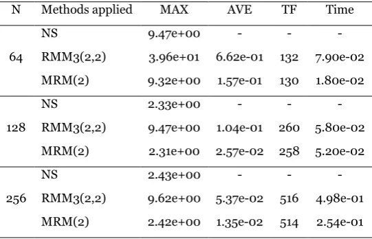
Table 1 and 2 display the comparisons between MRM and
existing rational methods of different order respectively. In
Table 1, we can see that the performance of the MRM(2) are
comparable to NS in terms of maximum and average error.
Meanwhile, as MRM is compared to RMM3 of the same order
in both tables, the proposed methods exhibit better accuracy
and efficiency of approximation as its time of execution and
total function function evaluation are smaller in value.
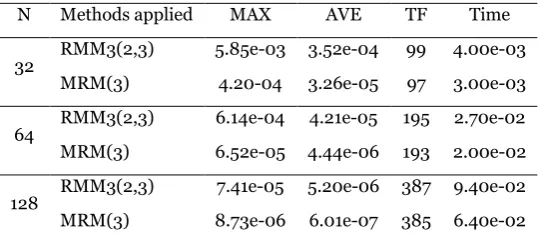
Table 3 and 4 portray the reliability of MRM in solving a
stiff problems as compared to teh existing methods. It can
be observed from the tables that MRM generates more
accurate approximation compared NS and RMM3 of the
same order based on displayed errors. Besides that, the
execution time and total function evaluation of MRM is less
than RMM3 indicating its efficiency in solving this problem.
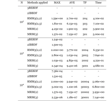
In Table 5, MRM is compared to RMM3 as well as some
BDF methods. From the table, we can see that the
maximum errors and average errors given by MRM are
Table 1. Comparison Between MRM(2) and Second Order Rational Methods for Solving Problem 1
N Methods applied MAX AVE TF Time
64
NS 9.47e+00 - - -
RMM3(2,2) 3.96e+01 6.62e-01 132 7.90e-02
MRM(2) 9.32e+00 1.57e-01 130 1.80e-02
128
NS 2.33e+00 - - -
RMM3(2,2) 9.47e+00 1.04e-01 260 5.80e-02
MRM(2) 2.31e+00 2.57e-02 258 5.20e-02
256
NS 2.43e+00 - - -
RMM3(2,2) 9.62e+00 5.37e-02 516 4.98e-01
smaller than the existing methods, which show that the proposed methods are capable in solving this problem. In terms
of time of execution, MRM took shorter time to finish an
execution compared to RMM3 of the same order.
VI. CONCLUSION
In this article, rational methods of second and third order are
introduced where the closest points of approximation is taken
into account in the derivation process. The proposed methods
are found to be A-stable, which indicates that they are suitable
in dealing with stiff equations. The numerical results presented in this research portray the capability of the
proposed methods in solving IVPs with singularity and
stiffness properties.
Table 2. Comparison Between MRM(3) and RMM3(2,3) for Solving Problem 1
N Methods applied MAX AVE TF Time
64 RMM3(2,3) 1.55e-03 2.61e-05 195 2.20e-02 MRM(3) 1.22e-04 2.06e-06 193 1.90e-02
128 RMM3(2,3) 1.20e-04 1.33e-06 387 4.00e-02 MRM(3) 2.93e-05 3.28e-07 385 1.69e-01
256 RMM3(2,3) 1.23e-04 6.84e-07 771 1.24e-01 MRM(3) 9.96e-05 5.53e-07 769 1.22e-01
Table 3. Comparison Between MRM(2) and Second Order Rational Methods for Solving Problem 2
N Methods applied MAX AVE TF Time
32
NS 1.78e-02 - - -
RMM3(2,2) 7.82e-02 2.42e-03 68 3.00e-03
MRM(2) 7.66e-03 3.21e-04 66 2.00e-03
64
NS 4.14e-03 - - -
RMM3(2,2) 1.78e-02 6.51e-04 132 1.70e-02
MRM(2) 2.70e-03 1.22e-04 130 1.60e-02
128
NS 1.03e-03 - - -
RMM3(2,2) 4.15e-03 1.75e-04 260 4.90e-02
MRM(2) 8.30e-04 3.79e-05 258 3.90e-02
Table 4.Comparison Between MRM(3) and RMM3(2,3) for Solving Problem 2
N Methods applied MAX AVE TF Time
32 RMM3(2,3) 5.85e-03 3.52e-04 99 4.00e-03 MRM(3) 4.20-04 3.26e-05 97 3.00e-03
64 RMM3(2,3) 6.14e-04 4.21e-05 195 2.70e-02 MRM(3) 6.52e-05 4.44e-06 193 2.00e-02
VII. ACKNOWLEDGEMENT
The authors would like to thank Universiti Putra Malaysia for
supporting this research under the Putra Grant
(GP-IPS/2018/9625300).
VIII. REFEREENCES
Abelman, S & Eyre, D 1990, ‘A Numerical Study of Multistep Methods Based on Continued Fraction’, Computers & Mathematics with Applications, vol. 20, no. 8, pp. 51-60. Fatunla, S 1982, ‘Nonlinear Multistep Methods for Initial Value
Problems’, Computers & Mathematics with Applications, vol.
8, no. 3, pp. 231-239.
Fatunla, S 1986, ‘Numerical Treatment of Singular Initial Value
Problems’, Computers & Mathematics with Applications, vol.
12, no. 5-6, pp. 1109-1115.
Ikhile, M 2001, ‘Coefficients for Studying One-Step Rational
Schemes for IVPs in ODEs: I’, Computers & Mathematics
with Applications, vol. 44, no. 3-4, pp. 769-781.
Lambert, JD & Shaw, B 1965, ‘On the Numerical Solution of y'= f (x, y) by a Class of Formulae Based on Rational
Approximation’, Mathematics of Computation, vol. 19, no.
91, pp. 456-462.
Lambert, JD 1973, Computational Methods in Ordinary Differential Equations, John Wiley & Sons, London, UK. Luke, YL, Fair, W & Wimp, J, 1975, ‘Predictor-Corrector Formulas Based on Rational Interpolants’, Computers & Mathematics with Applications, vol. 1, no. 1, pp. 3-12. Musa, H, Suleiman, M & Senu, N 2012, ‘Fully Implicit
3-Point Block Extended Backward Differentiation Formula for Stiff Initial Value Problems’, Applied Mathematical Table 5. Comparison Between MRM(2), MRM(3), RMM3 and Existing BDF Methods for Solving
Problem 3
N Methods applied MAX AVE TF Time
102
3BEBDF - - - -
2IBBDF - - - -
RMM3(2,2) 1.59e+00 2.70e-02 204 4.10e-02
RMM3(2,3) 1.81e-01 6.15e-03 303 7.10e-02
MRM(2) 4.25e-02 1.90e-03 202 3.90e-02
MRM(3) 1.37e-02 7.25e-07 301 5.00e-02
103
3BEBDF 1.24e-02 - - -
2IBBDF 1.50e-03 - - -
RMM3(2,2) 2.00e+00 3.77e-02 2004 6.53e-01
RMM3(2,3) 2.80e-03 1.03e-04 3003 7.64e-01
MRM(2) 1.03e-03 4.85e-05 2002 4.22e-01
MRM(3) 2.34e-04 9.41e-06 3001 4.68e-01
104
3BEBDF 7.36e-04 - - -
2IBBDF 1.51e-05 - - -
RMM3(2,2) 2.00e+00 3.94e-02 20004 5.06e+00
RMM3(2,3) 3.00e-05 1.10e-06 30003 6.80e+00
MRM(2) 1.57e-05 7.25e-07 20002 3.93e+00
Sciences, vol. 6, no. 85, pp. 4211–4228.
Musa, H, Suleiman, MB, Ismail, F, Senu, N & Ibrahim, ZB 2013,
‘An Improved 2-Point Block Backward Differentiation Formula for Solving Stiff Initial Value Problems’, In AIP Conference Proceedings, vol. 1522, pp. 211-220.
Niekerk, FV 1987, ‘Non-Linear One-Step Methods for Initial
Value Problems’, Computers & Mathematics with
Applications, vol. 13, no. 4, pp. 367-371.
Niekerk, FV 1988, ‘Rational One-Step Methods for Initial Value
Problems’, Computers & Mathematics with Applications, vol.
16, no. 12, pp. 1035-1039.
Okosun, KO & Ademiluyi, R 2007, ‘A Three Step Rational Methods for Integration of Differential Equations with
Singularities’, Research Journal of Applied Sciences, vol. 2,
no.1, pp. 84-88.
Okosun, KO & Ademiluyi, R 2007, ‘A Two Step-Second Order Inverse Polynomial Methods for Integration of Differential Equations with Singularities’,Research Journal of Applied Sciences, vol. 2, no. 1, pp. 13-16.
Ramos, H 2007, ‘A Non-Standard Explicit Integration Scheme for Initial-Value Problems’, Applied Mathematics and Computation, vol. 189, no. 1, pp. 710-718.
Ramos, H, Singh, G, Kanwar, V & Bhatia, S 2017, ‘An Embedded 3(2) Pair of Nonlinear Methods for Solving First Order Initial-Value Ordinary Differential Systems’,
Numerical Algorithm, vol. 75, pp. 509-529.
Ramos, H, Singh, G, Kanwar, V, & Bhatia, S 2015, ‘Solving First-Order Initial-Value Problems by using an Explicit Non-standard A-stable One-Step Method in Variable Step-Size
Formulation’, Applied Mathematics and Computation, vol.
268, pp. 796-805.
Teh, YY & Yaacob, N 2013, ‘A New Class of Rational Multistep Methods for Solving Initial Value Problem’, Malaysian Journal of Mathematical Sciences, vol. 7, no. 1, pp. 31-57. Teh, YY, Yaacob, N & Alias, N 2011, ‘A New Class of Rational
Multistep Methods for the Numerical Solution of First Order