Effectiveness of GPGPU for Solving the Magnetohydrodynamics Equations Using the CIP-MOCCT Method

E

ff

ectiveness of GPGPU for Solving the Magnetohydrodynamics

Equations Using the CIP-MOCCT Method

∗

)

Ryosuke UEDA, Yutaka MATSUMOTO, Masafumi ITAGAKI and Shun-ichi OIKAWA

(Received 5 January 2011/Accepted 22 April 2011)

A simple parallelization approach using General Purpose computation on Graphics Processing Unit was applied for solving the MHD equations using the CIP-MOCCT method. We investigated the efficiency of this parallelization approach and found that the computational speed of the modified code is significantly improved despite the simple modification.

c

2011 The Japan Society of Plasma Science and Nuclear Fusion Research

Keywords: MHD simulation, CIP method, MOCCT method, GPGPU, parallel computing DOI: 10.1585/pfr.6.2401092

1. Introduction

A method for the plasma dynamics analysis is numer-ical simulation by solving the MHD equations. However, solving them in three dimensions is expensive and requires excessive computing time; hence, faster processors are re-quired. Rapid improvement in Central Processing Units (CPUs) over the last several decades has enabled us to run larger and more accurate numerical simulations. The re-sults of these simulations have made great contributions to plasma and fusion research. The field of numerical sim-ulation has a high potential for future growth. Recently, however, there have been few CPU clock speed enhance-ments. Instead, CPU performance is increased using mul-tiple processors via the multi-core strategy. This indicates that further improvements of computing speed are obtained by parallel computation. Therefore, it will be necessary for us to employ the multi-core processor technology.

We are interested in using the Graphics Processing Unit (GPU) as a multi-core processor to perform parallel computations. The GPU is a multi-core processor devel-oped for graphics processing and affords massive parallel computations. In recent years, the high parallel perfor-mance of the GPU has motivated research outside graphics processing, i.e., general purpose computation; such tech-niques are called General Purpose computation on GPU (GPGPU).

GPGPU has been used in some simulation studies. In fluid dynamics, Brandvik and Pullan [1] solved two-dimensional (2D) and three-two-dimensional (3D) Euler equa-tions with uniform grids reducing the computational time by a factor of 29 (2D) and 16 (3D). Elsenet al.[2] solved 3D Euler equations on multi-block meshes. In plasma physics, Stantchevet al.[3] discussed the efficient imple-mentation of the particle-in-cell plasma simulation code. author’s e-mail: [email protected]

∗)_{This article is based on the presentation at the 20th International Toki}

Conference (ITC20).

Wang et al. [4] solved the MHD equations by using an adaptive mesh finite volume method. However, there are few studies on the application of GPU for solving the full MHD equations.

Because the experts in numerical simulations are not always experts in parallel computation, the approach in-volving GPGPU must be made simple to use. It is impor-tant for us to know the efficiency of a simple parallelization approach for solving numerical simulations. In the present study, we apply this approach to solve the MHD equations and investigate its efficiency.

For simple parallelization, an explicit scheme is con-venient, because the solution of simultaneous equations is unnecessary. We adopt a combination of the Constrained Interpolation Profile (CIP) [5], Method of Characteristics (MOC) [6], and Constrained Transport (CT) methods [7]; we call it the CIP-MOCCT method [8], which is an explicit scheme. The numerical phase errors of the advection equa-tion solved by the CIP method are smaller than those pro-duced by other schemes [9]. In addition, the CIP method can accurately follow the contact discontinuity and the boundary between the plasma and vacuum. This method has been used in a number of hydrodynamic [10] and MHD simulations [11, 12]. However, as mentioned in [13], the application of the CIP method to the MHD problems is difficult because of the traverse mode Alfv´en wave and the divergence-free condition of a magnetic field. Thus, a spe-cial treatment of the Alfv´en wave and the divergence-free condition is required. The MOCCT method is a standard technique for treating the Alfv´en wave and for satisfying the divergence-free condition. The CIP-MOCCT method is not used widely in the field of fusion science, but it has been employed in several astrophysics studies [14-19]. To the best of our knowledge, this is the first attempt to apply GPGPU to the CIP-MOCCT method.

c

2011 The Japan Society of Plasma

2. GPGPU and CUDA

Although performance improvements using GPGPU have been studied [20], GPU is essentially the hardware for graphics processing. In early studies employing GPGPU, programmers had to apply their algorithms and data struc-tures to the graphics programming model, which was not always straightforward, and hence, in-depth knowledge of graphics programming was required.

Compute Unified Device Architecture (CUDA) [21] is the development environment for GPGPU provided by NVIDIA. as NVIDIAr CUDATM_{. CUDA makes the} de-velopment of GPU computing applications much easier and more efficient than earlier attempts of using GPGPU. CUDA-C is an extension of the C Programming Language and is easy to learn for programmers with knowledge of C.

3. Implementation of CUDA

To calculate efficiently in CUDA, we have to appro-priately use the several types of memories on GPU, e.g., global memory, shared memory, constant memory, texture memory and register. In particular, the register and shared memory accessed via high bandwidths are essential for higher optimization, although these memories are difficult to use efficiently. For this reason, the optimization strat-egy involves the effectively use of these memories. On the other hand, although the access speed of the global mem-ory is low, it has much larger memmem-ory space and is easier to program compared with the shared memory. In this study, a computational code is modified via a simple paralleliza-tion approach using only the global memory.

In a parallelization approach, we need to find bottle-necks in the existing code. Such bottlebottle-necks were found in triple nested loops in our existing 3D MHD simulation code. In CUDA, the simplest parallelization approach for these loops is achieved by mapping each array element to the corresponding thread on the GPU (Fig. 1). This means that the number of threads invoked on the GPU is equal to the number of array elements. Because the shared memory is not used, this approach is not the best for optimization in terms of the calculation speed. However, it has major advantages: (i) we can easily modify the existing code and

Fig. 1 Mapping of each array element to the corresponding thread on the GPU.

List 1 Example of existing CPU code

List 2 Example of modified code

(ii) it is applicable to other numerical schemes.

List 1 shows the triple nested loop typically used in the 3D finite difference method in the computation on the CPU. In List 1, the elements of the 3D array are cal-culated while incrementing the indices i, j, and k of the triple nested loop. The modified version of the code in List 1 is shown in List 2. There are three functions

func, func kernel, andIDX. funcis executed on the CPU and callsfunc kernel, which is executed on the GPU. VariablesBLOCKSandTHREADSin parentheses,<<<

and>>>, are parameters specifying the number of threads run on the GPU. In the CUDA architecture, threads are arranged into threadblocks. BLOCKS andTHREADS indi-cate the number of threadblocks and the number of threads per threadblock, respectively. The product ofBLOCKSand

THREADSis the number of the total threads running on the GPU.func kernelis a “kernel function” invoked by the CPU and runs on the GPU. The processes performed in each thread are implemented in this kernel. Such kernel functions require a __global__ qualifier for their defi-nition. At the beginning of this kernel, the thread index

calcu-lated using built-in variablesblockDim, blockIdx, and

threadIdx. The indexidxcorresponds to the index of the array. We manipulate the 3D array as the 1D array in List 2. The functionIDXis invoked to obtain the index of the 1D array from the index of the 3D array. The__device__

qualifier is required for the functions executed on the GPU. In the present study, the modifications shown in List 2 have been implemented for all triple nested loops. As a result, these loops can be parallelized to be computed on the GPU.

4. MHD Equations and Numerical

Scheme in the Developed Code

4.1

MHD equations

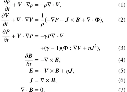
MHD equations in the developed code are expressed as follows.

∂ρ

∂t +V· ∇ρ=−ρ∇ ·V, (1) ∂V

∂t +V· ∇V= 1

ρ(−∇P+J×B+∇ ·Φ), (2) ∂P

∂t +V· ∇P=−γP∇ ·V

+(γ−1)(Φ:∇V+ηJ2), (3) ∂B

∂t =−∇ ×E, (4) E=−V×B+ηJ, (5)

J=∇ ×B, (6)

∇ ·B=0. (7)

Here,ρis the density,Vthe velocity,Pthe pressure,Jthe current density, Φthe viscosity stress tensor, Bthe mag-netic field, Ethe electric field,γthe ratio of specific heat andηthe resistivity.

4.2

CIP method

For fluid dynamics equations (1)-(3), we apply the CIP method [5], which is an explicit numerical technique applied to various problems, including fluid dynamics. In this method, a value and its derivative are treated as in-dependent physical variables. It enables us to accurately compute phenomena such as shockwaves, whose values change sharply in space.

4.3

CT method

The divergence-free condition of magnetic field B (Eq. (7)) does not appear in the time evolution equations (Eqs. (4)-(5)). It is pointed out that even small errors in sat-isfying the divergence-free condition cause artifacts such as a non-physical force parallel to the magnetic field [22]. In order to satisfy the above condition, the CT method [7] is adopted in the developed code.

Other schemes such as the projection scheme [22] re-quire a Poisson solver. Therefore, we also have to develop a Poisson solver that can use the GPU. On the other hand,

Fig. 2 Location of the physical variablesV,B, andEin the CT method.

the CT method enables the satisfaction of the divergence-free condition with the accuracy of the finite difference method by only definingV,B, andEon the staggered grid (Fig. 2).

4.4

MOC method

To compute the time evolution ofBby using Eq. (4), it is necessary to calculateEfrom Eq. (5). But in the stag-gered grid defined by the CT method, the variables ofV andBare not defined at the location of the variables ofE. Thus, it is necessary to interpolate the values ofVandB at the location of the variables of E. However, it is well known that numerical oscillation in the Alfv´en wave prop-agation is observed when the simple average ofVandB values at the location of the variables ofE is used. The MOC method [6] is used for the stable computation of the Alfv´en wave. From Eqs. (1), (2), and (4)-(6), a set of the characteristic equations are given by,

∂ ∂t +

Vx+ Bx

√_ρ

∂ ∂x Vy−

By

√_ρ

=0, (8)

∂ ∂t−

Vx− Bx

√_ρ

∂ ∂x Vy+

By

√_ρ

=0. (9)

These equations show thatVy∓By/√ρare constant on the characteristic lines and that the value ofVyandByatEzare obtained. In addition, other values of the components ofV andBat the locations of the variables of E are obtained similarly.

5. Comparison between CPU and

GPU

Fig. 3 Density profile att=0.1. The solid line is the solution of the CPU code. The squares are the solution of the GPU code.

Table 1 Specifications of GPU

GPU GTX285a _GTX480b

Total numbers of cores 240 480 Total amount of global memory 0.999 GB 1.499 GB Total amount of shared memory per block 16384 B 49152 B Total number of registers available per block 16384 32768 Clock rate 1.48 GHz 1.40 GHz

a_{NVIDIA Geforce GTX285} b_{NVIDIA Geforce GTX480}

setΔx = 1/200, Δt = Δx/10, γ = 2, andη = 0. The results att = 0.1 are shown in Fig. 3. It can be seen that the GPU solution is almost the same as the CPU solution. Moreover, these results also coincide with Brio-Wu’s re-sults. This proves the validity of our developed code.

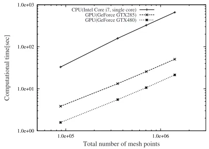
The performance of the modified 3D MHD simula-tion code using GPU in double precision was evaluated. The simulation settings were the same as for the above-mentioned MHD shock tube problem. We evaluated the CPU time from the start of the time integration (t = 0) until 100 time steps. Computational times using a CPU (Intelr CoreTMi7, 2.93 GHz) and two GPUs (NVIDIAr GeForcer GTX 285 and GTX 480) were measured. Al-though Intel Core i7 is a multi-core processor, the compu-tational time was measured for the case of using a single processor. The specifications of the GPUs are shown in Table 1.

The computational times measured for various mesh points are summarized in Fig. 4. It can be seen that for this calculation GTX285 is about 13 times faster than the CPU. Furthermore, GTX480 is about 30 times faster than the CPU. These results show the effectiveness of our sple parallelization using the GPU. This means that the im-provement in speed is independent of the total number of mesh points (NX×NY ×NZ). In addition, these results are independent of the problems, because the CIP-MOCCT method is an explicit scheme without a relaxation algo-rithm.

Fig. 4 Computational time using a CPU (Core i7) and two GPUs (GTX285 and GTX480). The horizontal axis is the total number of mesh points (NX×NY×NZ).

6. Summary and Discussion

We developed an MHD simulation code using the CIP-MOCCT method and modified it to extend its appli-cation to the parallel computing code using the GPU. Al-though we used a simple parallelization approach without utilizing the shared memory, the computational speed of the modified code was improved significantly.

The total memory on a GPU is smaller than that on a CPU. For this reason, increase in the number of mesh points lead to shortage in the GPU memory space. The use of multiple GPUs is considered a solution for this problem. However, the transfer of data between the CPU and the GPU or between computers in the multi GPU technique incurs large costs.

[1] T. Brandvik and G. Pullan, Proc. 48th AIAA Aerospace Sci-ences Meeting and Exbit, AIAA Press, 2008-607 (2008). [2] E. Elsen, P. LeGresley and E. Darve, J. Comput. Phys.227,

10148 (2008).

[3] G. Stantchev, W. Dorland and N. Gumerov, J. Parallel Dis-trib. Comput.68, 1339 (2008).

[4] P. Wang, T. Abel and R. Kaehler, New Astronomy15, 581 (2010).

[5] H. Takewaki, A. Nishiguchi and T. Yabe, J. Comput. Phys.

61, 261 (1985).

[6] J. Hawley and J.M. Stone, Comput. Phys. Commun.89, 127 (1995).

[7] C.R. Evans and J.F. Hawley, ApJ332, 659 (1988). [8] T. Kudoh and K. Shibata, CFD journal8, 56 (1999). [9] T. Tajima,Computational Plasma Physics: With Application

to Fusion and Astrophysics (Addison-Wesley, New York, 1989) Chap. 6.

[10] T. Yabe, F. Xiao and T. Utsumi, J. Comput. Phys.169, 556 (2001).

[11] N. Nishino, J. Plasma Fusion Res. SERIES6, 395 (2004). [12] R. Ishizaki and N. Nakajima, J. Plasma Fusion Res. SERIES

8, 995 (2009).

[13] Y. Matsumoto and K. Seki, Comput. Phys. Commun.179, 289 (2008).

[14] T. Kudoh and K. Shibata, ApJ476, 632 (1997b).

(1998).

[16] T. Kudoh, R. Matsumoto and K. Shibata, PASJ 54, 121 (2002a).

[17] T. Kudoh, R. Matsumoto and K. Shibata, PASJ 54, 267 (2002b).

[18] S.X. Kato, T. Kudoh and K. Shibata, ApJ565, 1035 (2002). [19] Y. Sofue, H. Kigure and K. Shibata, PASJ57, 39 (2005).

[20] J.D. Owens, M. Houston, D. Luebke, S. Green, J.E. Stone and J.C. Phillips, Proceedings of the IEEE96, 879 (2008). [21] NVIDIA CUDA Programming Guide.

[22] J.U. Brackbill and D.C. Barnes, J. Comput. Phys.35, 426 (1980).