Monitoring and Improving Managed Security
Services inside a Security Operation Center
Mina Khalili
1, Mengyuan Zhang
1,∗, Daniel Borbor
1, Lingyu Wang
1, Nicandro Scarabeo
2,
Michel-Ange Zamor
31Concordia Institute for Information Systems Engineering (CIISE), Concordia University, Montreal, QC H3G 1M8,
Canada
2University of Cassino and Southern Lazio, Viale dell’Università, 03043 Cassino FR, Italy 3Département d’informatique, Université de Sherbrooke, Sherbrooke, QC J1K 2R1, Canada
Abstract
Monitoring and improving the performance of Security Operation Centers (SOC) are becoming crucial due to the emerging need of benefiting from Managed Security Services (MSS) rather than hiring in-house security experts. In this paper, by observing workflows of a real-world SOC, a system consisting of three different modules is designed for monitoring analysts’ activities, analysis performance measurement, and performing simulation scenarios. The system empowers managers to evaluate the SOC’s performance, which helps them to conform to Service Level Agreement (SLA) and see the need for improvement. Moreover, the designed system is strengthened by a background service module to provide feedback about anomalies or informative issues for security analysts. Three case studies have been conducted based on real data collected from the operational SOC, and simulation results have demonstrated the effectiveness of the different modules of the designed system in improving the SOC performance.
Received on 28 November 2018; accepted on 19 December 2018; published on 25 January 2019
Keywords: Managed Security Services, Network Security Monitoring, Security Operation Center, Performance Metrics, Service Level Agreement, SLA, SOC, MSS, NSM, Security analysts
Copyright © 2019 Mina Khalili et al., licensed to EAI. This is an open access article distributed under the terms of the Creative Commons Attribution license (http://creativecommons.org/licenses/by/3.0/), which permits unlimited use, distribution and reproduction in any medium so long as the original work is properly cited.
doi:10.4108/eai.8-4-2019.157413
1. Introduction
Advantages of employing Managed Security Services (MSS), such as cost-effectiveness, skilled security experts, appropriate facilities, up to date security awareness, and 24 hours continuous service encourage different companies to outsource their security services rather than having in-house security employees [1]. Network security monitoring (NSM) is a service of MSS for continuous monitoring of networks by human experts instead of installing solely security appliances. The official definition of NSM is “the collection, analysis, and escalation of indications and warnings to detect and respond to intrusions” [2]. Therefore, in order to provide NSM service, Managed Security Service Providers (MSSP) deploy various sensors in the client site, such as Intrusion Detection Systems (IDS),
∗
Corresponding author. Email:[email protected]
to gather various suspicious alerts from each client’s computer network, and send them to the Security Operation Center (SOC). Then, SOC as a heart of NSM correlates and analyzes the alerts by its human security analysts to confirm whether they are successful exploits. A security incident is detected and confirmed by True Positive (TP) alerts as indications. In case of an incident, results of analysis need to be exposed to decision makers, in a process called escalation, to react in an appropriate way.
Emerging demand of outsourcing security services from different companies makes the business world increasingly competitive for MSS providers. Monitoring and improving performance of the SOC becomes more crucial to the managers to optimize their resources and improve the quality of their service.
activities. In order to have quantitative performance metrics, we need to carefully analyze analysts’ tasks, which is mainly a security investigation workflow, to model their behavior. Modeling the workflow should result in trackable and measurable actions. Task analysis techniques help extracting characteristics of human activities which would result in revealing the potential improvement options [3].
Monitoring the SOC performance lets the managers know if they conform to their SLA with their clients, if the number of analysts working in the SOC for each work-shift is enough to serve all the customers appropriately, how each analyst is working efficiently. Afterwards, with historical performance metrics on hands, managers can identify and assess the potential options to improve the current performance.
Challenges faced by the operational SOC include:
• To the best of our knowledge, there does not exist any model for the SOC analysis workflow to elaborate analysts’ detailed tasks. By modeling the analysis workflow, we can obtain a clear picture about analysis steps allowing the system to track analysts’ activities.
• Automated system for monitoring and evaluat-ing SOC performance are still lackevaluat-ing in exist-ing works. Consequently, there is no clear under-standing of SOC capability and different analysts’ performance.
• The study related to simulating potential improvement options of the SOC in order to assess their effectiveness stays neglected.
• A convenient knowledge transfer among analysts system is still missing. Analysts usually possess different knowledge, since they gain different knowledge during each investigation related to different clients.
The aforementioned challenges prevent managers to prioritize the efforts on improving SOC performance.
There are three main categories of related work (a more detailed review is given in Section 7). The first category discusses different aspects of MSS. Different designs for a SOC architecture, such as employing recognition mechanism of the immune system, cloud-based NSM, hierarchical mobile-agent-based approaches, etc, have been proposed [4–10]. Researchers study [11–13] various aspects of different operational SOCs to compare their functionality. However, these works are fundamentally different from our work, our study focuses on providing a solution for SOC managers to evaluate and improve SOC capability without modifying SOC architecture. The second category is alert correlation techniques helping to provide more accurate alerts, and reducing the rate of
False Positive (FP) [14–17]. The third category reviews studies about Call Centers (CC), since SOC and CC are similar regarding their performance evaluation. In a CC, operators answer to different calls in a queue, where in a SOC, analysts analyze incoming logs in a queue. Different queueing models are employed in this area to solve the problem of staffing, scheduling, and routing jobs policy [18–21]. To the best of our knowledge, there is little work related to performance measurement and improvement of a SOC.
In this paper, we propose a system to help managers by evaluating and monitoring the performance of a SOC and analysts by easing knowledge transfer among them. The designed system consists of a Graphical User Interface (GUI) for managers with three modules, monitoring, measuring, and simulation respectively. Additionally, a background service to generate feedbacks to SOC’s analysts about anomalies and informative issues are proposed to transfer knowledge among analysts. Monitoring module helps managers to obtain the current analysts’ activities of the SOC. This module illustrates details of recent investigations which are in progress or recently completed by the analysts. Managers can check overall and detailed SOC performance with the measuring module. Consequently, they can make the decision related to adding new analysts, recognize demanding clients, or optimize certain analysis steps average duration. With the simulation module, the managers can assess different performance improvement options to see the potential effect of each possible improvement on the performance result of real production data, without affecting the normal operation of the SOC. The simulation results also provide insight for the development team to improve SOC console applications and provide proof of concept for clients. Analysts benefit from the feedback module where they get hints about next probable steps. Feedbacks include the range of task times, the alerts for missing steps. Moreover, the knowledge of one analyst could be transferred to another one through the feedback module. Specifically, the contributions of our work are:
• First, we model the alert analysis workflow based on a real operational SOC.
• Second, we develop a practical system to monitor the analysis workflow, measure analysts’ perfor-mance based on divers perforperfor-mance metrics, sim-ulate possible improvement options and enable knowledge transfer among analysts by the feed-back module.
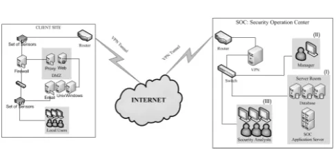
Figure 1. An example of a typical deployment model for Network Security Monitoring service representing an operational SOC and a client infrastructure
The rest of the paper is organized as follows. Sec-tion2describes the required background knowledge to understand this work. Section 3 illustrates our mod-eling methodology of the analysis workflow, and the logging phase of analysts’ activities. Section 4 pro-vides an overview of the system’s functionality, and the modules employed methodology. Section5 demon-strates the implementation of the whole system. Sec-tion 6 evaluates three case studies to assess different improvement options of the SOC performance. Sec-tion 7 reviews related work. Section 8 concludes our work and addresses the future work.
2. Preliminaries
In this section, the operational SOC workflow and its related characteristics and notations are explained to provide background knowledge. In this paper, our study is based on a real operational SOC. Besides illustrating SOC characteristics, a brief description of the designed system, and related definitions are given to show how the proposed system functions alongside the SOC main workflow.
Figure1illustrates a sample deployment model from an infrastructure perspective. The operational SOC uses Virtual Private Network (VPN) to connect the client site to the SOC. Sensors can be placed at various locations in the client network, such as outside the firewall facing internet, behind the firewall inside the demilitarized zone (DMZ), which are accessible internal points of client’s network from outside, or in the local network behind the firewall.
Analysts rely on SOC console, to review related alerts1 of each client and conduct the analysis. The workflow of alert analysis starts from the SOC consoleconsisting tasks, such as receiving alerts, cross-referencing network map of a client, examining a
1To clarify notations, alerts are specifically IDS-generated. However,
the event notation includes all kinds of machine-generated alerts and logs. Logs could be referred to normal operating system events (e.g., unsuccessful attempt to log in to a system) that can be useful for a security investigation.
client’s assets and vulnerabilities, opening content of the alert packet, and contacting the client in case of a true positive alert.
Incident category Investigation type Abbreviation
Security related BruteForce Attack BFA Denial Of Service DOS External Vulnerability Scan EVS
Malware Infection MI
Abnormal Activities AA
Others OTHERS
Policy violation Policy Violation PV Peer to Peer Bittorrent P2P
Table 1. List of investigation types related to the incident categories
There are eight investigation (the analysis task of sensor generated alerts by an analyst) types in two main categories from the SOC perspective, security-related incidents, and policy violation incidents. Table1 represents different investigation types.
For each investigation type, multiple approaches may exist. We collect all possible analysis approaches in one integrated model consisting of different investigation paths. The complete investigation workflow modeling phase will be described in details in Section3.1.
Sub-steps in each step are defined asactions. Actions are track-able points for each step performed by analysts. They correspond to single mouse clicks on the SOC console listed in Table3. To avoid discussing unnecessary details, we focus on steps rather than actions mostly throughout the paper.
3. Modeling and Logging the Investigation
Workflow
In this section, we demonstrate the modeling phase of the investigation workflow in Section3.1following with the logging phase of analysts’ activities in Section3.2.
3.1. Modeling the Investigation Workflow
The modeling of an investigation workflow is per-formed in two phases. The first phase is to gather the expert knowledge from analysts to identify different investigation types and relevant approaches. To model different tasks (steps) and their relationship, UML activity diagram has been employed to describe the model. The second phase is to visualize the model for the designed system. Graphviz V.2.38 [22] is employed to layout the activity diagram to represent the investi-gation workflow model in the system.
StepIDs Description
A Checking global view of the SOC Console which shows all alerts related to each client, expanding a specific alert to check the details and related destination and source IP addresses
B Classifying an event as not-suspicious and labeling it as FP
C Checking the network assets to see whether the reported alert is related to discovered vulnerabilities. Moreover, checking whether the same attack is reported recently
D Updating an existing incident for the client, since a similar incident is reported recently. Or updating the incident description, since the client responded to the incident (clarifying the incident)
E Creating a new incident for the client, since indications confirm the alert as suspicious (true positive alert) F Checking the escalation grid for the related client. In
this grid, analysts are provided information about how the client prefers to be informed about different kinds of attacks depends on criticality (e.g. call, email, report) O Opening the alert packet content by a specific tool to
analyze deeply, such as Wireshark.
Table 2. Step IDs and their description
Step ActionID Description
A 130 Opening a specific client alert view 105 Expanding the aggregated alert detail 107 Clicking on the alerts to view alert details
by “Editor”
B 109 Clicking on the button “Acknowledge” from alert detail
125 Clicking on the button “Acknowledge” from alert list
C 104 Clicking on “View Asset” that will open a small window from source IP
126 Clicking on “View Asset” that will open a small window from destination IP 110 Clicking on the tab “Incidents” 112 Clicking on “Edit incident” to open and
view the incident
D 114 Clicking on the button “Add to incident” 116 Clicking on the button “Add alerts to
incident”
117 Under comment box, clicking on the button “Apply” or “OK”
E 119 Clicking on the button "Create incident" 121 Clicking the button "Finish"
F 122 Opening the documents dashboard 123 Selecting the client
124 click on the document "Escalation Grid" O 103 clicking on the button "Export to pcap"
127 Opening the packet using Wireshark
Table 3. Steps with sub-steps as Action IDs and related description
The logical relationship among different nodes of the model could be AND or OR. By traversing a single investigation path in a model, all existing nodes in the same path have AND logical relationship and in different investigation paths are described as OR relationship. AND logical relation implies mandatory nodes. If an analyst misses one mandatory node between previous and next node of a path, the feedback module will warn the analyst about the missing steps. A detailed discussion related to feedback module is in
Figure 2. An Example of an Investigation Model
Sections4.1, and5.4. In a model, we use diamond shape to indicate OR relationship. Different investigation paths can be followed based on different conditions, such as different investigation types.
3.2. Logging Analysts’ Activities
Based on the extracted model from Section 3.1, each task is defined by different actions as single mouse clicks on the SOC console. These mouse clicks are logged automatically in our system. Each log resembles one single action performed by an analyst through the SOC Console. Our data gathering process follows extract, transform, load (ETL) process; this section mainly focuses on the data extraction and section 6.1 completes the data processing.
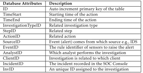
Database Attributes Description
ID Auto increment primary key of the table TimeStart Starting time of the action
TimeEnd Ending time of the action InvestigationTypeID Related investigation type StepID Related step
ActionID Related action
SourceID Event (alert) comes from which source e.g., IDS EventID The rule identifier of sensors to raise the alert AnalystID Which analyst performs the investigation ClientID Investigation is related to which client IncidentID The incident recorded in the SOC Console InvID An unique ID assigned to the investigation
Table 4. Database table attributes and description
Each row of logs consists of eleven attributes, which are described in Table 4. For example, the start and end time of the action as two attributes: TimeStart, and TimeEnd. Based on the identified actions through the SOC Console, the logging script captures the actions started and ended via the SOC Console. The start time of actions are bound to the specific buttons, and end time of actions are bound to the start time of the next recognizable action by the system. In this way, no time in the middle of an investigation is skipped in case of using other tools not being monitored by our logging system. End time of the last action is a specific button to close an investigation. A tuning step is required to adjust the logs during the pre-processing phase before storing the logs into the database, which will be demonstrated in Section6.1.
As is shown in Table 4, each row of activity logs has related StepID and ActionID which the row will be matched to the investigation model. Therefore, by extracting StepID:ActionID from a log, we can map the nodes from our model to the logs. By tracking analysts activities, our system is able to understand the process in each investigation, such as the analyst is working on which step currently, or what is the next action. Mapping all logs of one investigation to the model, the system can also identify the missing steps to alert analysts.
Table 5 shows a sequence of logs belonging to one investigation, containing three steps and eight actions (A:130ÝA:105ÝC:104ÝC:110ÝA:107ÝE:119ÝC:112
ÝE:121). This investigation path is illustrated in the
model shown in Figure 2 as specified by the double boxes. By comparing the combined key of each log, which is StepID:ActionID, the system can map the log to a node of the model (the analyst is performing which step and action). By looking at all logs and mapping them to related nodes in the investigation model, we can see which path is followed by the analyst. Furthermore, By identifying the path followed by an analyst in the model, the feedback module can notify analysts about probable next steps or missing steps (will be discussed in Section5.4).
4. Methodology
In this section, we elaborate the system modules and their functionalities. Then, we describe the methodology and detailed implementation of each module.
4.1. Overview of The System
The designed system assists both managers and analysts as a value-added component of the SOC Console. General workflow of the designed system is shown in Figure 3, where activity logs are being gathered from analysts’ machines and stored in the database. The main GUI including the monitoring, the measuring, and the simulation modules keeps reading the database and provides different capabilities to the managers. The feedback module works as a background service to give feedback to analysts in real time.
Generally,the monitoring moduletracks and monitors analysts’ activities.The measuring moduleallows man-agers to check SOC’s performance with divers metrics provided by the system. Furthermore, customizable Online Analytical Processing (OLAP) analysis is inte-grated into the system to provide more detailed analysis performance results. The simulation module facilitates evaluating improvement options through two diff er-ent approaches: first, studying the impact of analysis duration by modifying the duration of analysis steps. second, applying a different queuing model and alert dispatching approach to evaluate the overall perfor-mance.The feedback moduleassists analysts of the SOC by notifying them with different information through the Microsoft Windows operating system tray, while they are performing investigations through the SOC Console.
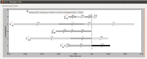
Monitoring Module. Figure 4 shows the monitoring
module of the managers’ GUI. This module is provided to illustrate the detailed information of the SOC ongoing investigations in an easy-to-understand way. The main purpose is to visualize the ongoing investigations. The GUI keeps only the investigations started within a predefined period (e.g., 30 minutes).
ID TimeStart TimeEnd In
v
estig
a
tionT
ypeID
S
tepID
A
ctionID
SourceID Ev
en
tID
Anal
ystID
Clien
tID
Inciden
tID
InvID
203547 1432954820387 1432954834974 MI A 130 0 33906 4 15 0 1210176 203548 1432954834974 1432954851571 MI A 105 0 33906 4 15 0 1210176 203549 1432954851571 1432954857971 MI C 104 0 33906 4 15 0 1210176 203550 1432954857971 1432954868877 MI C 110 0 33906 4 15 0 1210176 203551 1432954868877 1432954934995 MI A 107 1 33906 4 15 0 1210176 203552 1432954934995 1432955078419 MI E 119 0 33906 4 15 0 1210176 203553 1432955078419 1432955083059 MI C 112 0 33906 4 15 500204 1210176 203554 1432955083059 1432955083059 MI E 121 0 33906 4 15 500204 1210176
Table 5. Log entries of one investigation related to MI investigation type
Figure 3. The proposed system architecture
Figure 4. The monitoring module dashboard
stacked bar is an ongoing investigation in the SOC. A vertical line, represents the current time, separates the investigation into two phases. The left side of the vertical line demonstrates the completed steps of an investigation, and the right side indicates the next predicted steps. The prediction of the steps is provided by mapping the ongoing investigations to their relevant models, which will be detailed in section 5.1. The visualized investigations get updated by reading new data from database incrementally. For example,PV1 in Figure4, the analyst finished the step A and is doing the step O, and the predicted step is continuing on the step O with demonstrating historical average time (0m48s).
Measuring module. We propose the measuring module
in order to have a better understanding of the performance of the SOC. Qualitative measurement
usually is ignored as it is difficult or expensive to be scaled. However, in our system, the measuring module provides managers with quantitative measurements of the SOC performance.
To the best of our knowledge, this work is one of the first studies related to SOC analysis performance in the literature. Jacobs et al. [12] examine different aspects of three real-world operational SOCs. The performance metric in their work only counts the number of analyzed incidents per analyst for each day. However, without taking the time duration of analysis into consideration, counting the number of incidents solely is not a good metric. The efforts on difficult investigations will not be properly captured. As a result, analysts are not motivated to analyze carefully, since it results in showing lower productivity for them in managers’ point of view. In a university SOC assessed in the same work, a ticketing system dispatching alert tickets to analysts, provides a performance metric, which is time spent on each ticket, however, the detailed study is missing. To address the existing works’ limitation, our measuring module is designed to provide various SOC’s performance metrics to evaluate SOC behavior.
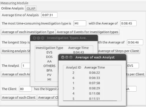
We enumerate the metrics provided by the measuring module. Important results, such as the maximum values, are shown in the main GUI, where detailed analysis is reachable through different buttons. Figure5 shows the measuring module dashboard, and the two detailed analysis reports are open in separate windows. The first group of metrics provides average analysis time from different perspectives. More specifically,
• Total average analysis time.
• Average analysis time of each investigation type/analyst/client.
Figure 5. The measuring module dashboard
• Average analysis time of different investigation types for the same client.
• Average analysis time of different analysts for the client.
The second group of performance metrics concen-trates on the average duration of different investigation steps. This group attempts to show steps’ average dura-tion in general, for different analysts and clients. More specifically,
• Ranking analysis steps according to the time spent in executing.
• Average analysis time of different analysts for the same step.
• Average analysis time of different clients the same step.
The third group is about showing maximum values for selected performance metrics in the managers’ GUI. This group helps managers to determine if maximum values significantly differ from historical average durations. For example,
• Identifying which investigation type takes more time to be analyzed.
• Which step of which investigation type takes more time to be analyzed.
• Which analyst has the highest average time for which investigation type.
• Which client has the highest average time for which investigation type.
• Which analyst has the highest average time for which client.
The fourth group is the number of created and updated incidents for different parameters. For exam-ple,
• The number of created and updated incidents for each investigation type.
• The number of created and updated incidents for each analyst.
• The number of created and updated incidents for each client.
OLAP Component An OLAP tool is employed beside
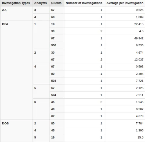
the designed measuring module inside the managers’ GUI. OLAP empowers managers to create new analysis queries with mouse dragging and clicking instead of modifying code or writing complicated SQL queries. An open-source web-based OLAP engine, Community Edition Saiku (CE Saiku) [24], is integrated into the GUI providing customized data analysis opportunities. CE Saiku is implemented by Pivot4J Java API using Mondrian OLAP server. We integrate web-based Saiku to the managers’ desktop GUI by embedding a browser. Saiku configuration for SOC performance metrics is discussed beside an example in section5.2.
Simulation Module. The simulation module is designed
to show the effects of potential changes on the investigation workflow. It simulates the effect of a change on real activity logs, and recalculates performance metrics. It helps the managers to prioritize efforts on potential improvements of the SOC. Two potential changes as simulation options are provided. One is modifying the current steps’ duration, and the other is changing the dispatching method of alerts.
Figure 6. The results of the simulation module alongside the measuring module
The second simulation capability is simulating the dispatching phase of incoming alerts among analysts with a different queueing model. Different ways of dispatching services (alerts) among servers (analysts) are usually studied as queuing models [25]. In our work, a different alert dispatching method is simulated to assess the employed approach effect on the SOC performance metrics.
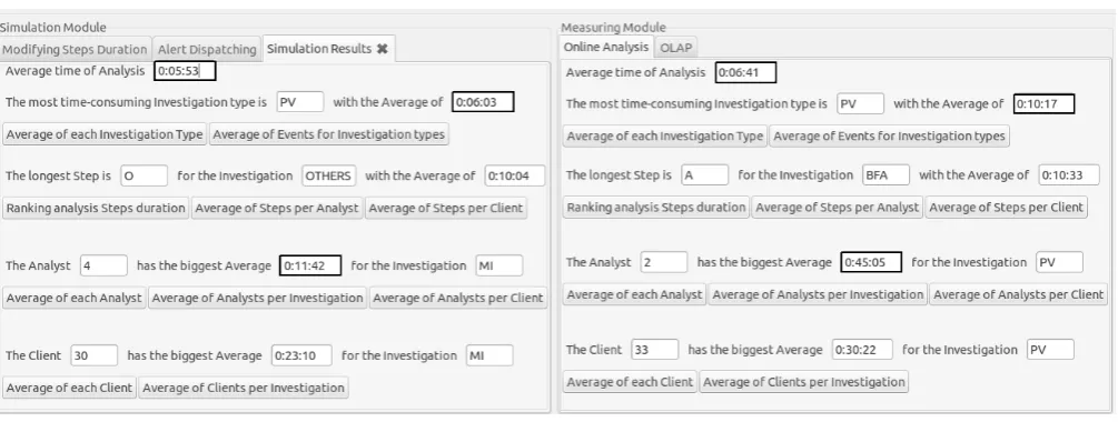
The result of both simulation scenarios is shown side by side with the real one (measuring module) in the GUI to ease the comparison process for managers. Figure6shows an example of the provided simulation results beside the measuring module. In this way, comparing the effect of the simulation scenario on actual SOC performance metrics is easy for the managers. For instance, as we see in Figure 6, the simulation reduces the average time of analysis from 6:41 to 5:53. By the measuring module results, we see the most time-consuming investigation type is PV with the average of 10:17, the conducted simulation reduces it to 6:03 however the investigation type is not changed. Moreover, we can compare easily that the biggest investigation type average duration belongs to AnalystID 2 for PV with the average of 45:05, and this simulation changes it to AnalystID 4 for MI with the average of 11:42.
Feedback Module. The feedback module is designed for
knowledge transfer among SOC analysts. Knowledge can be a hint about next required action to proceed in the investigation, notifying the analyst about anomalous durations and missing steps, or showing the result of previous similar investigation types performed by other analysts. The analysts are firstly notified about mentioned information in the Windows operating system tray, and the summary of all notifications are accessible in a desktop GUI.
The feedback Module works as a background service uninterruptedly as analysts activity logs are being stored in the database. It keeps reading the database, and mapping them to the investigation model. As a result, the system can notify analysts about next probable steps, find anomalies, and warn analysts about them. The module reminds the analyst what is the probable next step based on the step he is currently performing. Anomaly notifications are about spending normal duration on the steps, or not missing an action. For instance, If the analyst takes 50% (which is configurable) less or more time than the historical average duration of the step, he will be warned. If the analyst’s activities do not match one of the investigation model’s paths, he will receive a warning about the missing steps.
previous analyst’s investigation, can take a faster action with the knowledge of the previous analyst.
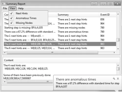
The feedback module is shown in Figure 7. As is shown, different hints are provided to the analyst. The analysts receive notifications in real time about their ongoing investigations in the Windows operating system tray, where all notification reports are accessible by the GUI.
Figure 7. The feedback module notifications and reports
5. Implementation
In this section, the methodology and implementation details of each module are discussed. All modules are implemented in Python 2.7 programming language and existing libraries.
5.1. Monitoring Module
Visualization of the monitoring module is implemented with Matplotlib package [26] in Python. In each update, the module fetches StepID and ActionID from the last log of the investigation, and composes the mapping key. Then, it maps the key value to the relevant node of the investigation model. By traversing the investigation model, it can recognize what is the next probable action. If the next node is End, it shows the investigation is completed, otherwise it shows the next probable action and step. If the predicted steps contain multiple possible actions, a black-color step will display on the GUI otherwise a white-color step will show.
5.2. Measuring Module
The measuring module is designed to provide SOC performance statistics with different metrics. The SOC performance metrics are described in Section 4.1. By having the measurable investigation workflow, performance metrics can be calculated by running
SQL queries on the database. The duration of an investigation is measurable from provided analysts’ activity logs with different attributes. In our system, we use PostgreSQL [27] in the implementation to support SQL standard queries.
Saiku OLAP Configuration. CE Saiku is integrated into
the managers’ GUI to the measuring module to provide easy customizable metrics on the investigation logs. Leveraging this open source OLAP tool allows us to connect directly to the developed system relational database, which is PostgreSQL, access data easily, and design the desired multidimensional schema by mapping database tables fields to cubes. The package we use to integrate CE Saiku browser into the desktop GUI is CEF python [28]. In this way, the managers can work with CE web Saiku application through the GUI directly.
The multidimensional OLAP schema, Mondrian [29], is defined in an XML format to be used by CE Saiku engine. It is designed by considering multiple attributes of analysts’ activity logs to provide detailed investigation measurement to the SOC managers. The attributes considered for the schema are: investigation types, analysts, and clients. Quantitative attributes in the calculation include TimeStart, TimeEnd, and InvID. For each quantitative attribute, we need to set a proper calculation function, called aggregator. For example, a sum function could be set to TimeStart and TimeEnd attributes resulting in a total investigation duration. The calculation function for InvID counts the number of distinct values indicating how many investigations are done.
A schema is designed by considering multiple attributes of analysts’ activity logs to provide detailed investigation measurement to the managers. The attributes considered for the schema are: investigation types, analysts, and clients. Quantitative attributes in the calculation include TimeStart, TimeEnd, and InvID. For each quantitative attribute, we should set a proper calculation. For example, a sum calculation could be set to TimeStart and TimeEnd attributes. The calculation for InvID counts the number of distinct values.
Figure 8. Partial OLAP analysis results
5.3. Simulation Module
The simulation results only provide a hypothesis evaluation for end users; the production database stays the same. The alert dispatching simulation is provided in a replicated database by storing the simulated logs, and the modifying steps’ duration simulation is performed by SQL queries in real time.
Modifying Steps’ Duration. Performance metrics are
calculated based on modified time durations as a comparison to the measuring module. The goal of this modification is to obtain the possible steps for automation and significantly reduce human effort in the analysis.
Alert Dispatching Method. The default alert dispatching
method is assigning the same number of clients to the available analysts of a work shift. Analysts are responsible for their assigned clients and work independently. For instance, we have five available analysts and 15 clients, every three clients are assigned to one analyst regardless of any consideration. This approach has some pitfalls, such as the possibility of assigning clients with a high load of alerts to the same analyst, where the other analyst is assigned clients with a low load of alerts. It is also possible that two clients assigned to the same analyst are under attack at the same time, and the analyst cannot handle both of them at the same time, where none of the clients of the other analyst are in such a critical situation.
The simulation methods follow a single-queue, multiple-servers methodology. Considering several servers serving clients from a single queue is known as
theM/M/cmodel wherecis the number of servers [25]. The discipline in these systems is first-come, first-served and the arrival rate of jobs is based on the Poisson process. And the job routing method is Fastest Server First [30], which distribute the incoming jobs to the fastest server first.
In this simulation, two metrics will be provided to assess the effect of the simulated method. One is the average analysis duration, and the other is the alert waiting time. The waiting time is the time the alert stays in the SOC console (queue) to be analyzed. It is the subtraction of the start time of an investigation from the arrival time of an alert in the queue. In our study, waiting time implies the response time of the SOC to incidents which is an important factor for the managers to respect SLA for different clients. By considering the waiting time, we can also assess how the new approach would affect the waiting time of the alerts. The simulation will be detailed in a case study in Section6.4.
5.4. Feedback Module
The feedback module first maps analysts’ activity logs back to the investigation model to locate the analysis step. Then, it provides the predicted steps to analysts as hints for the possible solutions. In the end, it tracks the analysts’ activities and provides notifications for missing steps.
The first algorithm to find missing steps maps analysts’ incoming activity logs to the investigation model continuously to see whether a step is missed. It starts checking logs of one investigation from the first log. It checks every two successive logs (adjacent) in the database to see whether they are also successive in the model. If they are not adjacent in the model, there are one or more missing nodes between them. The second algorithm is to find the shortest path between two nodes. Since it is possible to have several paths between two nodes, the shortest path, including fewer nodes, is selected to report missing actions or steps. The first algorithm provides the accurate missing steps, while the second algorithm consumes less computation time and provides the least missing steps.
In order to report duration anomalies, as some analysts may not spend enough time on some steps, a dynamic duration standard is provided base on historical data for each specific step. The standard duration is considered as real-time average of historical data in a range, as follows.
(1−n)∗AverageDuration < StandardDuration <(1 +n)∗AverageDuration (1)
between 48 and 72. The alternative range percentage is configurable.
6. Data Processing and Case Studies
Three case studies are elaborated in this section to show the effectiveness of our designed system in improving the SOC performance. Firstly, we go through the dataset pre-processing and provide different statistics of the dataset. Then we provide case studies.
6.1. Dataset Pre-processing
A pre-processing step is implemented to remove data-gathering mistakes resulting in out-of-range values, impossible data combinations, and missing values.
Out of range values implies those steps’ durations, which are too long compared to real durations and need to be normalized. One possible reason for these abnormal cases is that the TimeEnd of each action is considered as TimeStart of the next action. Therefore, the gap (e.g., analysts take a leave) between sequential actions will increase the duration. Such a large duration between steps is considered as noise in our dataset. Similar to the noise removal, we clean the data from the attributes missing values, conflicting actions, and false positive or contextual events.
Different activity logs from analysts’ machines are gathered and stored at the same time by the logging script. Firstly, different analysts’ activity logs are separated from each other and ordered by time. Then, different investigations from the same analyst are distinguishable from each other by a specific ActionID (#130). Then we assign each investigation a unique identifier as InvID.
TimeStart TimeEnd Inv
estig
a
tionT
ypeID
S
tepID ActionID
SourceID Ev
en
tID
Anal
ystID
Clien
tID
Inciden
tID
1432357758628 1432357765749 0 1 130 0 0 2 10 0 1432357765749 1432357822688 0 1 105 0 0 2 10 0 1432357822688 1432358143981 1 1 107 0 34463 2 10 0 1432358143981 1432358146472 0 16 103 0 0 2 10 0 1432358146472 1432358250989 0 16 127 0 0 2 10 0 1432358250989 1432358250989 1 2 125 0 34463 2 10 0
Table 6. Raw activity logs in the format of text file
InvestigationTypeID and StepID values are mapped from numbers to predefined codes of the system in the pre-processing phase. For instance, in the text file, value 1 for the InvestigationTypeID attribute is an identifier of Policy Violation (PV) investigation type. Consequently, those numbers are mapped to the abbreviated forms of their investigation type names. Similarly, it is done for StepID attribute, codes 1, 2, 3, ... are mapped to A, B, C, ... respectively.
Parameters New Updated Closed Total Incidents Incidents Alerts Dataset Number of log entries 3301 1558 9380 14239
Number of investiga-tions
194 331 765 1290
Proportion 15.04% 25.66% 59.3% 100%
Total average analysis duration
17:52 06:41 05:16 07:32
Average duration of fastest analyst
12:10 03:59 04:44 06:22
Average duration of slowest analyst
22:38 09:46 11:27 11:52
Table 7. The dataset statistics
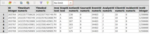
In Table6, we can see values of InvestigationTypeID attribute are zero and one, firstly all values of this attribute are changed to one. Then all values are mapped to PV as we see in Figure9. If all those values related to the InvestigationTypeID were zero, it would mean the InvestigationTypeID was not retrievable. We will simply assignOTHERSto the investigationTypeID.
Figure 9. Rows of logs related to one investigation placed in the database
6.2. Statistics of Dataset
The time period of the dataset is from June 2015 to August 2015 for 57 days. 6 analysts perform alert analysis for 40 clients. The time duration format in Table 7, and all following tables is mm:ss. As is shown, 40.7% of investigations result in creating or updating incidents, where 59.3% of total investigations are about closing alerts after an investigation. Average analysis duration of investigations ending in creating new incidents is 17:52, while the average duration of updating an incident and closing an alert are 06:41, 05:16, respectively. Moreover, different analysts have different average analysis durations. The slowest analyst’s average duration is 11:52 whereas the fastest one is 06:22.
Inv New Updated Closed Total Type Incidents Incidents Alerts Dataset
- # Avg # Avg # Avg # Avg
EVS 6 20:50 11 06:28 91 03:27 108 04:43
MI 47 20:31 68 07:04 183 06:22 298 08:45
BFA 24 20:18 17 08:38 102 05:16 143 08:11
PV 20 19:46 10 10:17 80 05:41 110 08:40
AA 6 19:27 2 01:10 67 05:25 75 06:25
DOS 4 17:35 5 08:13 77 04:55 86 05:41
OTHERS 87 15:02 218 06:17 165 04:58 470 07:26 Table 8. The dataset statistics regarding different investigation types. Here, average values are time duration in the format of mm:ss, and the other column (#) is the number of instances.
AA, DOS, and OTHERS. Most popular attack type is MI with 47 distinct incidents in the dataset, whereas DOS has the least number of created incidents, 4. After MI, other two popular attack types are BFA and PV. Since the number of cases for OTHERS type is much more than other known categories, it is not mentioned in our comparisons for known investigation types.
For almost all investigation types, the average time of updating an incident is more than closing the alert of the same type. An exception is the AA type whose number of related cases (#2) for updated ones is not enough to be considered as a counterexample. However EVS attack type takes more time to be confirmed as an incident, the average duration of getting closed is the least (03:27) among other types. The most time-consuming investigation type for updating an incident is PV type, which is reasonable as it mostly needs communicating with the client to clarify the situation.
Looking at the total dataset statistics, MI, BFA, and PV are the most time-consuming alert types in the SOC regardless of the investigation result. The number of received alerts from these attack types is highest beside EVS, although EVS alerts are analyzed quickly. The trend shows MI type has the highest number of investigations (298), and the highest average analysis time (08:45).
6.3. Case Study I, Modifying the Duration of Steps
This case study is about assessing potential steps which could be automated to improve overall performance. Every change in a system needs to be assessed before going into production. After going through all steps that analysts perform for an alert investigation, two possible automation options are recognized. One is about checking clients’ assets and the other is about checking escalation grid. These two are considered as potential improvements to the current investigation workflow.
Checking clients’ assets (part of step C). In this case
study, we assess how the possible solution would affect the SOC performance. As we know, investigations can
Inv Type Dataset Average Simulation Average Reduction Ratio
EVS 20:50 18:17 12.24%
MI 20:31 18:15 11.05%
BFA 20:18 19:22 4.6%
PV 19:46 19:25 1.77%
AA 19:27 16:13 16.62%
DOS 17:35 16:57 3.6%
OTHERS 15:02 14:01 7.62% Table 9. Class: creating new incidents; 94 out of 194 investigations (48.45%) contain step C. By the simulation, the total average analysis duration decreases from 17:52 to 16:31, or 7.55%.
Inv Type Dataset Average Simulation Average Reduction Ratio
EVS 06:28 05:10 20.10%
MI 07:04 06:24 9.43%
BFA 08:38 06:47 21.43%
PV 10:17 09:08 11.18%
AA 01:10 00:30 57.14%
DOS 08:13 08:13 0.0%
OTHERS 06:17 06:04 3.45% Table 10. Class: updating incidents; 42 out of 331 investigations (12.69%) contain step C. By the simulation, the total average analysis duration decreases from 06:41 to 06:13, or 6.98%.
result in three different categories, creating a new incident, updating the current incident, or closing the alert as FP. For the first two categories (creating or updating incidents), the simulation is done in a way that the related actions’ duration to asset checking is eliminated completely, then average analysis durations are recalculated to show the improvement. For the closing alerts category containing this step, careful observation is made whether the reason for closing the alert was about mismatching asset’s vulnerabilities and the raised alert. If the condition is true, we claim the entire investigation is useless. Implementing this solution would remove this FP automatically. As a result, FP alert reduction aside, analysts’ time would be saved. If the alert is not closed immediately after checking this step, we just deduct this step duration from the duration.
Creating a new incident Table 9 shows the results
Inv Dataset Average after Final Reduction Type Average eliminating inv Simulation Ratio
EVS 03:27 03:28 3:11 8.17%
MI 06:22 06:14 5:44 8.02%
BFA 05:16 05:19 5:01 5.64%
PV 05:41 05:55 5:36 5.35%
AA 05:25 05:08 4:59 2.92%
DOS 04:55 04:55 4:46 3.05%
OTHERS 04:58 04:50 4:35 5.17% Table 11. Class: closing alerts; 5.36% of investigations are removed, 231 out of 724 investigations (31.9%) are involved in this simulation. By the simulation, the total average analysis duration decreases from 05:12 to 04:54, or 5.77%.
Closing alerts category The step for checking a
client’s asset is performed in 30.2% of investigations (231 out of 765 investigations) which can be eliminated from the analysis process similar to other two investigation categories scenarios. Specifically, 41 out of 231 (17.75%) alerts of these investigations are closed immediately after checking the step indicating useless investigations. Since they are closed immediately after this step, it is assumed that the raised alerts did not match the assets vulnerabilities. As a result, they could be cleaned from the alerts repository before reaching analysts’ SOC Console. By implementing the solution, the rate of false positive alerts would be decreased by 5.36% (41 out of 765) in this class, where 266 minutes of analysts time (around four and a half hours) would be saved. For the remaining 190 investigations containing this step, we eliminate the asset checking step and recalculate the results for the closing alerts category. Results are shown in Table 11 illustrating 7.28% decrease in the total average analysis duration.
All investigation categories Table12 illustrates
dif-ferent simulated average analysis durations for different investigation types. After removing 41 investigations from the closed alerts category, 29.38% of investigations are affected by this scenario, and the total average analysis duration decreases by 6.83%. The most affected attack types are EVS, MI, and BFA, where PV and DOS attacks are improved to a lower degree.
Considering investigation classes, the summary of simulation results is shown in Table13.
Checking escalation grid (step F). One analysis step is
checking escalation grid to find out how the related client should be informed in case of a new or updated incident. Each client’s escalation grid as an informative document is accessible through some mouse clicks in the SOC Console. The contacting approaches can be different for each client based on the severity of the incident and the client’s preference.
A possible improvement for this step is providing information about the required escalation method for
Inv Dataset Average after Final Reduction Type Average eliminating inv Simulation Ratio
EVS 04:43 04:46 4:15 10.84%
MI 08:45 08:49 7:58 9.64%
BFA 08:11 08:19 7:42 7.41%
PV 08:40 08:59 8:36 4.27%
AA 06:25 06:11 5:47 6.47%
DOS 05:41 05:44 5:33 3.2%
OTHERS 07:26 07:26 7:03 5.16% Table 12. Total dataset; 29.38%, 367 out of 1249 investigations contain step C (41 investigations are removed from 1290 total investigations, as is discussed for the closed alerts category). By the simulation, the total average analysis duration decreases from 07:34 to 07:03, or 6.83%.
Inv Dataset Simulation Involved Reduction Class Average Average Proportion Percentage Creating
new inci-dents
17:52 16:31 48.45% 7.55%
Updating inci-dents
06:41 06:13 12.69% 6.98%
Closing alerts
05:12 04:54 31.9% 5.77%
Total dataset
07:34 07:03 29.38% 6.83%
Table 13. The summary of simulation results for different investigation classes
an incident in the window of creating and updating incidents in the SOC Console. By correlating related client escalation grid and related incident type, the proper contact approach can be fetched and shown to the analyst as a hint which saves him time to go through different buttons to find out the required information. In this scenario, we observe how frequent this step is beside the average duration analysts spending on it.
We found that 58 out of 194 (29.9%) investigations contain checking escalation grid for the category of creating incidents. Besides, 18 out of 331 (5.44%) and 23 out of 765 (3.0%) investigations include checking escalation grid for the categories of updating and closing incidents respectively. Since the number of involved investigations for the last two investigation classes is not much (as expected), the simulation is only done for the creating new incidents category. Table14 shows the detailed simulation results for the class of creating new incidents, where the related step is eliminated completely. Our simulation illustrates the average investigation duration is decreased by just 1.3%. MI and AA attack types are mostly checked for the proper escalation method.
Combination of two possible improvements. By combining
Inv Type Dataset Average Simulation Average Reduction Ratio
EVS 20:50 20:36 1.12%
MI 20:31 20:06 2.03%
BFA 20:18 20:06 0.98%
PV 19:46 19:43 0.25%
AA 19:27 19:01 2.23%
DOS 17:35 17:28 0.66%
OTHERS 15:02 14:52 1.11% Table 14. Class: creating new incidents; 58 out of 194 investigations (29.9%) contain step F. By the simulation, the total average analysis duration decreases from 17:52 to 17:38, or 1.3%
Inv Dataset Average after Simulation Reduction Type Average eliminating inv Average Ratio
EVS 04:43 05:18 04:46 10.06%
MI 08:45 09:46 08:48 9.9%
BFA 08:11 08:59 08:18 7.61%
PV 08:40 09:32 08:59 5.77%
AA 06:25 06:40 06:11 7.25%
DOS 05:41 05:59 05:43 4.46%
OTHERS 07:26 07:52 07:25 5.72% Table 15. Combined effect: 41 investigations are removed resulting in an increase in the average analysis durations shown in the third column, 377 out of 1249 investigations (30.18%) are affected by the combination of two simulation scenarios, and decreases the total average analysis duration from 8:09 to 7:33, or 7.36% beside saving four and a half hours man-hour.
assets’ vulnerabilities and automated shown escalation grid together are simulated to show the effect on the averages. Table15shows the simulation results. Firstly, by removing 41 investigations which were closed immediately after checking assets’ vulnerabilities, new analysis averages are shown in the second column indicating on an increase which means removed investigations were part of short investigations. Then by eliminating the steps related to checking assets and escalation grid, simulated average analysis durations are calculated and shown in the fourth column. By employing both automation solutions, the total average analysis duration would be decreased by 7.36%. The most affected attack types are EVS and MI.
6.4. Case Study II, A Different Alert Dispatching
Method
In this case study, the simulation of a different dispatching method of incoming alerts among analysts is assessed. As discussed in Section5.3, the simulation follows single-queue, multiple-servers methodology, where the routing strategy is assigning alerts to the fastest analysts.
The number of analysts working in the SOC is different from one work-shift to another work-shift. For
weekdays (Monday to Friday), there are three work-shifts per day; day-shift from 8:00 to 16:00, evening-shift from 16:00 to 00:00, and night-evening-shift from 00:00 to 8:00.
In total, 33-day work-shifts are considered for the simulation with the minimally two analysts working per work-shift. For 17 work-shifts, two analysts are working per work-shift. For 15 work-shifts, three analysts and for one work-shift four analysts are working in the SOC in parallel. Table 16 shows statistics on the selected dataset for 33-day work-shifts and simulation results. Each column represents one investigation class, such as new incidents which the first sub-column is dataset average analysis time, the second one is simulated average analysis time, and the third sub-column is the reduction ratio.
By comparing Table7with Table16, we can see the proportion of the closing alerts category increases from 59.3% to 94.12%, since all investigations of the work-shift are considered regardless of their duration.
The simulation result in Table16represents the effect of the simulated dispatching approach on the total average analysis time and waiting time of different investigation classes and the total dataset. Total average analysis duration and waiting time of the total dataset are improved by 4.42% , and 2.18% respectively.
6.5. Case Study III, The Feedback Module
Our study on the analysts’ activity logs shows investigations’ average durations for different attack types are usually different from each other. Different analysts’ average durations are usually also different even for the same attack type implying the different efficiency. The different efficiency can be due to the analysts’ different levels of knowledge regarding analysis approaches or familiarity about clients’ environments.
As is discussed in Sections4.1and 5.4, one feature of the feedback module is showing previous investigation logs whose alert type is similar with which the analyst is currently analyzing. In this case study, we evaluate how such a feedback module would affect the analysts’ performance.
We consider one analyst as the senior analyst who has better efficiency than others. The other analysts who may benefit from the senior analyst’s knowledge and experience are called junior analysts. We model the trend of investigation durations of the senior analyst, and partially apply the model to future investigation durations of the junior analysts, assuming that, since the junior analysts can see what the senior analyst performed through the feedback module, they can potentially improve their efficiency.
Inv classes New Incidents Updated Incidents Closed Alerts Total Dataset # of log
entries
1059 731 11181 12971
# of
investigations 75 163 3807 4045
Proportion 1.85% 4.03% 94.12% 100%
Parameters Real Simu % Real Simu % Real Simu % Real Simu % Total average
analysis duration
18:13 16:54 7.23% 05:19 04:16 19.75% 01:25 01:25 0% 01:53 01:48 4.42%
Waiting time 120:16 116:02 3.52% 120:00 116:02 3.3% 120:06 117:34 2.11% 120:06 117:29 2.18% Table 16. The alert dispatching method dataset statistics for 33-day work-shifts, the simulation results and the reduction ratios.
AnalystID Average Variance The Number of Investigations
1 16:05 - 1
2 01:17 - 1
3 21:34 717.72 2
4 05:46 100.57 5
5 07:29 35.45 6
6 03:16 7.85 45
Table 17. Different analysts’ statistics; the average investigation duration, the variance of investigations durations, and the number of investigations related to EventID 101010 which is a custom EventID for verifying DNS queries.
regression analysis, the mathematical function repre-senting investigation durations is extracted from the dataset. The duration of each investigation completed by the senior analyst is considered as a data point for that analyst. Different data points of the analyst is ordered by time chronologically as they are per-formed in different days. By extrapolating the estab-lished model, we can predict future investigation dura-tions of the senior analyst based on his historical data.
A realistic assumption here is that the junior analyst will partially benefit from the knowledge of the senior analyst by observing the latter’s investigation details but such benefit is not likely sufficient to enable the former to perform those analyses with exactly the same efficiency as the latter. In other words, knowledge transfer is partial instead of complete. Accordingly, we assign a percentage range by which a junior analyst can improve the efficiency of his/her investigations of the same type after observing the senior analyst’s approach and results. It is assumed in this case study that a junior analyst can gain 10% to 60% of the senior analyst’s knowledge to improve his investigations. To obtain a more accurate estimation of such a range from real data is a future work.
The average investigation duration of a junior analyst for EventID 101010 is considered as the default value for his/her future investigation durations in our simulation. This default value can be improved by learning from the senior analyst. For example, when we assume the junior analyst gains knowledge by
10%, his average investigation duration is calculated as the summation of 90% of the estimation proportion (90%∗Junior_Investigation_Average) and 10% of the
senior analyst’s investigation duration (as predicted by the model) (10%∗Model_Investigation_Duration). As
another example, when we assume the junior analyst gains knowledge by 60%, his average investigation duration is equal to 40% of his own duration plus 60% of the senior analyst’s duration.
The reason behind considering the average investi-gation duration of the senior and junior analysts in this case study instead of modeling their investigations durations is that we do not have sufficient data points to establish the model for them. Since the dataset does not provide enough investigations for any single EventID, the average investigation duration is considered. Since the dataset does not provide enough investigations for any single EventID, the average investigation duration is considered for the junior analysts.
For the regression analysis, the X-axis represents time series ordering investigations chronologically and the Y-axis is the investigation duration for the data points. In practice investigations might be performed on the same day or across different days in the period of the dataset, but the time distance between data points considered in this case study is limited to one day in this simulation. We aim to obtain the main trend of the investigation durations in chronological order as either an increase or decrease in the average investigation durations of the senior analyst during the dataset period.
There turn out to be a lot of fluctuations for the 45 data points representing investigation durations for the AnalystID 6. To smooth the curve, every five adjacent investigation durations are averaged and represents one data point. In the end, we obtain a model of the senior analyst’s investigation durations as the exponential equation shown below.
y= 2.8352e−0.005x (2)
senior analyst, and the next 10 data points are the extrapolation of the model. The average duration of the dataset data points is 3:04, where the average duration of the extrapolated data points is 2:37 showing the decreasing trend of the senior analyst’s model, which indicates that the analyst’s efficiency for this type of investigations slowly improves over time.
X; Time Y; Investigation X; Future Y; Extrapolated Series Duration Time Series Investigation Duration
1 2:11 11 2:41
2 2:20 12 2:40
3 2:11 13 2:40
4 5:57 14 2:38
5 3:31 15 2:38
6 2:32 16 2:37
7 1:59 17 2:36
8 2:54 18 2:35
9 5:46 19 2:35
10 1:16 20 2:34
Table 18. First 10 investigation durations represent data points from the dataset for the senior AnalystID 6 and EventID 101010, and the next 10 investigation durations are extrapolated under the model.
As is discussed, in order to estimate the junior analyst’s efficiency, a percentage range of gaining knowledge is considered from 10% to 60%. We simulate 10 future investigation durations for the junior analysts by combining their own investigation average duration and the effect of the senior analysts knowledge using the percentage.
Table 19 shows the simulation results, where the junior analyst is AnalystID 5 with the default investigation average duration of 7:29. Estimation results show that, if the junior AnalystID 5 gains 10% of the senior analyst’s knowledge through the feedback module, the average investigation duration will change from 7:29 to 6:59, decreased by 6.68%. If he/she gains 60% of the senior analyst’s knowledge, his/her average investigation duration will change from 7:29 to 4:33, decreased by 39.2%.
Table 20 shows the simulation results where the junior analyst is AnalystID 4 with the default average of 5:46. Simulation results show that, if the junior AnalystID 4 gains 10% of the senior analyst’s knowledge, the average investigation duration will change from 5:46 to 5:26, decreased by 5.78%. If he/she gains 60% of the senior analyst’s knowledge, his/her average investigation duration will change from 5:46 to 3:53, decreased by 32.66%.
In summary, in this case study, the impact of showing previous investigations to the analysts, which is one of the important features of the feedback module, is assessed based on some assumptions. The AnalystID 6 is considered as a senior analyst, and AnalystsIDs 5 and 4 are juniors. Based on the simulation results, if
Simulated Junior’s average Model’s inv Simulated Time Series inv duration*90% duration*10% inv duration
1 6:44 0:16 7:00
2 6:44 0:16 7:00
3 6:44 0:16 7:00
4 6:44 0:15 6:59
5 6:44 0:15 6:59
6 6:44 0:15 6:59
7 6:44 0:15 6:59
8 6:44 0:15 6:59
9 6:44 0:15 6:59
10 6:44 0:15 6:59
Simulated Junior’s average Model’s inv Simulated Time Series inv duration*40% duration*60% inv duration
1 2:59 1:37 4:36
2 2:59 1:36 4:35
3 2:59 1:36 4:35
4 2:59 1:35 4:34
5 2:59 1:35 4:34
6 2:59 1:34 4:33
7 2:59 1:34 4:33
8 2:59 1:33 4:32
9 2:59 1:33 4:32
10 2:59 1:33 4:32
Table 19. The simulation results of the feedback module’s impact for the junior AnalystID 5 with the default average investigation duration of 7:29 for the EventID 101010. The first part simulates the junior’s efficiency for 10 future investigations by considering the knowledge transfer percentage as 10%, and the second part simulates the junior’s efficiency for 10 future investigations by considering the knowledge transfer percentage as 60%.
the junior analysts gain 10% to 60% of the professional analyst’s knowledge; the efficiency of AnalystID 5 can be improved by 6.68% to 39.2%, and the efficiency of AnalystID 4 can be improved by 5.78% to 32.66%. Those results clearly demonstrate the potential benefit of the feedback module of the system. The summary of results is shown in Table21.
7. Related Work
In this section we first review the existing work regarding MSS, MSM, NSM, and SOC in Section 7.1, then the literature of alert correlation techniques are presented in Section 7.2. Finally, we illustrate the studies related to CC in Section7.3.
7.1. MSS, MSM, NSM, SOC
Simulated Junior’s average Model’s inv Simulated Time Series inv duration*90% duration*10% inv duration
1 5:11 0:16 5:27
2 5:11 0:16 5:27
3 5:11 0:16 5:27
4 5:11 0:16 5:27
5 5:11 0:16 5:27
6 5:11 0:16 5:27
7 5:11 0:16 5:27
8 5:11 0:15 5:26
9 5:11 0:15 5:26
10 5:11 0:15 5:26
Simulated Junior’s average Model’s inv Simulated Time Series inv duration*40% duration*60% inv duration
1 2:18 1:37 3:55
2 2:18 1:36 3:54
3 2:18 1:36 3:54
4 2:18 1:35 3:53
5 2:18 1:35 3:53
6 2:18 1:34 3:52
7 2:18 1:34 3:52
8 2:18 1:33 3:51
9 2:18 1:33 3:51
10 2:18 1:32 3:50
Table 20. The simulation results of the feedback module’s impact for the junior AnalystID 4 with the default average investigation duration of 5:46 for the EventID 101010. The first part simulates the junior’s efficiency for future 10 investigations by considering the knowledge transfer percentage as 10%, and the second part simulates the junior’s efficiency for future 10 investigations by considering the knowledge transfer percentage as 60%.
Junior Default Investigation Estimation Reduction AnalystID Average Duration 10% - 60% 10% - 60%
5 7:29 6:59 4:33 6.68% 39.2%
4 5:46 5:26 3:53 5.78% 32.66%
Table 21. The summary of results
Bejtlich [2] provides a formal definition for NSM with different terms and security processes beside deploy-ment considerations. Shin and Gu [6] implement NSM for cloud services in which the CloudWatcher frame-work is proposed to direct netframe-work packets of the cloud passing through defined network security monitoring points. Ballard et al. [9] propose OpenSAFE to focus the monitoring on routing network traffic. OpenSAFE pro-vides configurable network traffic routing by employing OpenFlow-supported devices [34] to preserve high line rates performance, and introduces ALARMS as a flow specification language to ease the management of net-work monitoring devices.
Various researchers are working on proposing a new framework for SOCs. Bidou [4] discusses the main concepts and components of a SOC as a heart of NSM for the first time. Different modules’ functionalities, from event generating, collecting, and storing to analysis approaches and related response methods, are covered to explain the process of building a SOC,
where integrating all modules is considered as a challenge. Niu et al. [5] propose a solution to utilizing recognition mechanism of the immune system to detect intrusions. Hu and Xie [8] present a novel design for a SOC by applying Dempster-Shafer Theory to the basic SOC model proposed by Bidou [4]. In this work, the authors claim to reduce TP and TN by using multi-sensor data fusion techniques. Later, Li et al. [7] propose a hierarchical mobile-agent-based SOC to avoid one fixed location for alert correlating and improve computational efficiency.
Several works are done related to enhancing the performance of SOC. Tsai et al. [35] introduce a mechanism for trusted sharing of security incidents among independent SOCs. Ganame et al. [10] develop a SOC providing a global view of the monitored network in a graphical way to help analysts detecting attacks. Jacobs et al. [11] propose a classification model to assess SOC services. In the proposed framework, either SOC clients or owners can measure the maturity of SOC processes regarding certain aspects, e.g, log collection. Michail [13] studies SOC from a business perspective and proposes answers for permanence related questions in SOC. Sundaramurthy et al. [12] study three operational SOCs to understand the functionality details by an anthropological approach. However, to the best of our knowledge, there is no work presenting a clear approach to model the SOC analysis process by human analysts, and evaluating SOC performance by different metrics in the literature.
7.2. Alert Correlation Techniques
Two SOC-related studies, which are done by Bidou. [4], and Hu and Xie. [8] claim that correlating gathered events from different sensors plays an important role to generate accurate suspicious events, and reduces the rate of false positive. There are plenty of works for alert correlation, since it is considered as the most improvable and effective part of a SOC regarding performance improvement.
Luo and Kay. [36], and Hall and Llinas. [37] have employed data fusion techniques earlier in other fields either military or non-military intelligent systems. Leau et al. [38] have conducted a survey, and classified alert correlation approaches to four categories; correlation methods based on similar semantics in alerts description, predefined attack scenarios, preconditions and postconditions of attacks, and data mining.
by employing attack graphs which are predefined attack scenarios. By introducing a novel approach Queue Graph, nested loop based correlation is solved, and it is possible to match alerts to related nodes of the attack graph. Zali et al. [16] presents a correlation approach by pre-defining simple relations among minor attacks to identify attack scenarios in real time.
A correlation method is introduced by Zhu and Ghor-bani [39] to recognize different attack scenarios without experts’ knowledge background. Multilayer perceptron and support vector machine are employed as neutral network approaches to evaluate correlation probability of each pair of alerts. Correlation probability estimation results are stored in Alert Correlation Matrix, which will be used to extract high-level attack scenarios.
Ramaki et al. [17] present a correlation framework to detect multi-step attack scenarios in real time as an Early Warning System (EWS). An EWS aims to identify hidden risky behavior of a system which might expose the system to threats [40]. Statistical and stream mining (sequence analysis) techniques are employed to design the correlation scheme.
7.3. Call Centers And Queuing Models
In both SOC and CC, humans serve different clients with various service requests in a queue. In the SOC, security analysts are the servers and incoming alerts are considered as different service requests, whereas in the CC, operators respond to different calls. In both cases, incoming service requests are coming in a queue and the service needs to meet certain service level agreement (SLA) specified between clients and service company.
Brown et al. [41] describe queuing-theoretic models for service systems based on a basic common queuing model M/M/N system or Erlang-C [42] which considers arrival rate based on the Poisson process. Green et al. [18] study the different methods of queuing-theory for setting a service system to serve clients whose request-pattern is predictable during a day (how much demanding in which periods).
Excoffier et al. [19] propose a solution to solve the staffing problem, which determines the minimum number of servers that could conform to SLA. The proposed solution is based on linear approximation, and considered arrival rate as random. Mattia et al. [20] presents a robust solution guaranteeing that the proposed shift schedule with the minimum number of servers can conform to SLA. It computes the solution by considering the probability distributions of uncertain parameters.
Other recent works related to queuing models of CC [21, 43] focus on considering impatient customers as a new input parameter for queuing models. This new
parameter introduces the uncertainty from the client side into the models.
8. Conclusion and Future Work
In this section, we conclude our work by summarizing the contributions in Section 8.1 and discussing the directions of future work in Section8.2.
8.1. Conclusion
In this paper, by modeling the main workflow of an operational SOC, a system for improving the SOC’s performance has been designed consisting of four modules, monitoring, measuring, simulation, and feedback. The integration of the first three modules provide SOC managers a solution to evaluate the current performance, and assess potential improvement options through simulations. The feedback module enables knowledge transfer among SOC analysts in their ongoing workflows to improve their performance. By deploying a logging component inside the main SOC console, analysts’ activity logs from a real production SOC are collected from June to August 2015 for 57 days in a dataset for evaluating our system. Three case studies have been conducted based on the dataset to study the designed system’s effectiveness, namely, modifying the duration of steps, a different alert dispatching method, and the feedback module’s impact.