An Improved Spectral Clustering Algorithm Based on Local Neighbors in Kernel Space

An Improved Spectral Clustering Algorithm

Based on Local Neighbors in Kernel Space

1

Xinyue Liu1,2_{, Xing Yong}2 _{and Hongfei Lin}1

1 _{School of Computer Science and Technology, Dalian University of Technology,}

116024 Dalian, China

2 _{School of Software, Dalian University of Technology,}

116620 Dalian, China xyliu@dlut.edu.cn

Abstract. Similarity matrix is critical to the performance of spectral clustering. Mercer kernels have become popular largely due to its successes in applying kernel methods such as kernel PCA. A novel spectral clustering method is proposed based on local neighborhood in kernel space (SC-LNK), which assumes that each data point can be linearly reconstructed from its neighbors. The SC-LNK algorithm tries to project the data to a feature space by the Mercer kernel, and then learn a sparse matrix using linear reconstruction as the similarity graph for spectral clustering. Experiments have been performed on synthetic and real world data sets and have shown that spectral clustering based on linear reconstruction in kernel space outperforms the conventional spectral clustering and the other two algorithms, especially in real world data sets.

Keywords: Spectral Clustering, Kernel Space, Local Neighbors, Linear

Reconstruction.

1.

Introduction

In recent years, spectral clustering has become one of the most popular clustering algorithms due to its high performance in data clustering and simplicity in implementation compared to the traditional clustering methods. It is based on the spectral analysis methods and solves the data clustering by graph partitioning problems [1], [2]. Spectral clustering algorithms consist of two steps: (1) construct a similarity graph with some kind of similarity function; (2) find an optimal partition of the graph and cluster the data points. The former which reflects the intrinsic structure of the data plays an important

1 _{This paper is supported by “the Fundamental Research Funds for the Central}

role in spectral clustering [3], [4], thus a great deal of effort has been carried out to address it [5], [6].

Spectral clustering makes use of information achieved from an appropriately defined affinity matrix. Its primary strength is the ability to treat complex patterns where traditional methods (such as

k

-means) either cannot be applied, or fail. The similarity matrix should be built in such a way that reflects the topological characteristics of the data sets. The most commonly used similarity measure is Gaussian function which is defined as

2 2

2 || || ) ,

( 

j i x x

j i x e x G

 

 , where

x

_i and

x

_j represent two point respectively [7]. Although Gaussian function is simple to implement, the selection of the parameter



is still an open issue. Generally it is non-trivial to find a good



and spectral clustering is sensitive to the value of



, especially in a multi-scale data sets. In practice,



is often set by an empirical value, such as it is set as 0.05 of the maximal pair wise Euclidean distance among the data points in normalized cut algorithm [2]. What’s more, sparsity is another desired property, since it can offers computational advantages [7].

In this paper, we focus on how to construct an optimal similarity graph. We propose a novel method to obtain the similarity matrix based on linear reconstruction with local neighbors in kernel space. The idea of linear reconstruction derives from the manifold learning which assumes data points are locally linear and each point can be reconstructed by a linear combination of its neighbors [8]. It has been applied to semi-supervised learning [9] and spectral clustering [10]. The kernel method has become popular largely due to many successes in applying kernel methods such as kernel PCA [11] and spectral regularization [6]. In our algorithm, we introduce the kernel methods for constructing the similarity matrix which increase the linear separability by mapping the data into high dimensional space. Experimental results on both artificial data sets and real world data sets indicate that spectral clustering based on local neighborhood in kernel space (SC-LNK) outperforms the traditional spectral clustering (SC), self-tuning spectral clustering (SSC) and locality spectral clustering (LSC).

The rest of this paper is organized as follows: some related work is discussed in Section 2. We begin with a brief overview of NJW method [12] in Section 3. Then introduce the method of linear reconstruction in Section 4 and mercer kernel in Section 5 on details of constructing the similarity matrix for our algorithm. In Section 6, we summarize our algorithm and experimental results are then presented in section 7. Finally we conclude the discussions and point out further works in the last section.

2.

Related Work

how to construct an optimal similarity matrix for spectral clustering [6], [13], [14]. Most existing works on constructing similarity matrix were built on Gaussian kernel function which is limited to its sensitive scale parameter and the real world data in some situation. Little attention has been paid to the other methods to measure the similarity in spectral clustering.

As mentioned above, the scale parameter of Gaussian function is very sensitive, especially in data sets with multiple scales. In order to deal with the problem, Manor et al. [13] proposed a new algorithm called self-tuning to use a local scale parameter for each data point, i.e., they use the distance of

k

-th nearest neighbor of each point as -the scale parameter. The parameter

k

is set to 7 in their experiments. However, as have shown in our experiments, it fails on many real data sets although performs well on some synthetic data sets.

Gong et al. proposed a spectral clustering method [10] which called LSC algorithm. Instead of using the pairwise relationship, they considered the linear neighbors relationship based on the idea of local linear embedding in manifold learning [8]. With this novel relationship in hand, LSC achieved the similarity matrix which represents the local neighbors information well. In particular, the matrix obtained is sparse which offers computational advantages. However, the LSC method has some limitations in synthetic and real world data sets as shown in our experiments.

In [15], the linear Reconstruction in kernel space had been described. DeCoste et al analysis the local linear embedding technique in kernel space and applied to specific application. Through the introduction of kernel methods, it can increase the linear separability by mapping the data into high dimensional space. Therefore, the kernel trick method conduces to deal with the multiple and real data sets. But the authors only focus on the classification problem.

3.

Review of Spectral Clustering

Give a set of data points X {x1,x2,...,xn} with each point

d

i R

x  , then we

can construct an undirected graph

G



(

V

,

E

)

in which every vertex

v

_i represents the data point

x

_i. According to a similarity function, we obtain the similarity graph and let W be its weighted adjacency matrix. Note that

0 

ij

w and

W

is symmetric. Each edge

(

i

,

j

)



E

carries a weight

w

_ij

4.

Analysis of Linear Reconstruction

The similarity graph plays an important role in a spectral clustering algorithm. Before, we need to define a similarity function on the data. In the common case, a reasonable candidate is the Gaussian similarity function, which is

defined as 2

2 2 || || ) , (  j i x x j

i x e

x G

 

 . However, it indicates that there is no reliable way to choose the parameter



when there are very few or even there are no labeled examples according to [18].

Instead of using pairwise relationship to construct the similarity graph in conventional spectral clustering, we propose to use the neighbor information of each point to construct the graph.

Algorithm 1: Normalized Spectral Clustering Input: Data set X, number

k

of clusters Output: A partitioning

S

1

,

S

2

,



,

S

_k

begin

Construct similarity matrix nn R

W 

Define a diagonal matrix





 n

j W i j j

i D

1 (, ) )

,

(

Form the normalized Laplacian matrix 2 1 2 1 _



D WD L

Compute the

k

largest eigenvectors of

L

and

construct the matrix

U



R

nk with the eigenvectors as its columns

Form matrix

Y



R

nk from

U

by normalizing the rows to norm 1.

Group

Y

into clusters

S

1

,

S

2

,



,

S

_k with

k

-means

end.

For convenience of calculation, we assume the sample space is locally linear, that is, each point can be optimally reconstructed by a linear combination of its neighbors [8]. Then our objective is to minimize

2 ) ( :

||

||





_



i j N x

x

j ij j

i

w

x

x



₍₁₎

where N(x_i) represents the neighbors of

x

_i, and w_ij is the contribution of

j

x to x_i . According to [8], w_ij should satisfy the constraint

0 , 1 ) ( :  



jxjNxi ij ij

w

w . Intuitively, the more similar

x

_j to

x

_i, the larger w_ij

would be. Thus we can use

w

_ij to measure the similarity between

x

_j and

i









   

















) ( , : , ) ( , : , 2 ) ( : 2 ) ( :

)

(

)

(

||

)

(

||

||

||

i k j i k j i j i j x N x x k j ik i jk ij k i T j i x N x x k

j ij ik

j i x N x j ij x N x

j ij j i i

w

C

w

x

x

x

x

w

w

x

x

w

x

w

x



(2)

where

C

i_jk represents the

(

j

,

k

)

-th entry of the local Gram matrix at point x_i

and

C

_jki



(

x

_i



x

_j

)

T

(

x

_i



x

_k

)

. Then we can obtain the reconstruction weights

of each data point by solving the following

n

standard quadratic programming problems

0

,

1

.

.

min

) ( : ) ( , : ,









  i j i k j ij x N x

j ij ij

x N x x k j ik i jk ij w

w

w

t

s

w

C

w

(3)

Using the above method, we will construct a sparse matrix

W

. It is worth mentioning that we set the weights

W

_ij



w

_ij and

W

_ji



w

_ij. If there are any overlap, the later weight will overlap the former one so that we can guarantee the symmetric of the reconstruction matrix

W

. Then the

W

can be treated as the similarity matrix.

5.

Kernelized Linear Reconstruction

5.1. Mercer Kernel

Combining the kernel method can optimize the performance of clustering algorithm [19], [20]. Through the introduction of kernel methods, it can increase the linear separability by mapping the data into high dimensional space. DeCoste has analyzed the linear Reconstruction in kernel space [15]. Consider a

l



D

matrix

X

of data points. A mercer kernel K(xi,xj) will

projects two given points from

D

-dimensional original space into some (possibly infinite-dimensional) feature space and return their dot product in that feature space. That is

)

(

)'

(

)

(

)

(

)

,

(

x

_i

x

_j

x

_i

x

_j

x

_i

x

_j

where



is some mapping function which need not explicitly to compute the coordinates of the projected vectors. Thus the kernel method can avoiding curse of dimensionality when explored large non-linear feature spaces.

One of the most popular mercer kernels is the radial basis function (RBF) kernel: 2 2 2 || ||

)

,

(

 v u

e

v

u

K

 



(5)

where the parameter



controls a scale of the dot product of the two data points. We will use this kernel when mapping the input space to its feature space.

5.2. Linear Reconstruction in Kernel Space

In general, the selection of

k

nearest neighbors use the Euclidian distance in original space. In this paper, we use the distance based on Mercer kernels. The distance between data point

x

_i and

x

_j in kernel space is defined as:

)

||

)

(

)

(

(||

))

(

),

(

(

2 j i j i

ij

dist

x

x

x

x

d















(6)

Through Mercer kernel, distances can be calculated directly from kernel value as follows

jj ij ii

ij

K

K

K

d





2



(7)

For each (x_i) in kernel space, denote its

k

nearest neighbors in kernel

space as N(



(xi)), then the kernelized reconstruction error is:

2 )) ( ( ) ( :

(

)

||

)

(

||





_



i

j N x

x

j ij j

i

w

x

x

_{ }







(8)

To find the optimal weights for reconstructing, we must compute the covariance matrix

C

_jk in kernel space which is:

))

(

)

(

(

))

(

)

(

(

_{i j} T _{i k}

i

jk

x

x

x

x

C















(9)

Then replacing each resulting term of form



(x_a)



(x_b) in Eq. (4) with the

corresponding kernel value K_abK(x_a,x_b). The kernelized covariance matrix can be obtained by

)

(

,

_{k i}

j

x

N

x

x





i _{ii ij ik jk}

jk

K

K

K

K

We can compute the weights matrix

W

of kernel space and use it as the similarity matrix for spectral clustering.

6.

Proposed Algorithm

In this section, we will introduce our algorithm called spectral clustering algorithm based on local neighbors in kernel space (SC-LNK). The main procedure of SC-LNK is summarized in Algorithm 2.

Algorithm 2: The SC-LNK Algorithm

Input: Data set X, number

k

of clusters Output: A partitioning

S

₁

,

S

₂

,



,

S

_k

begin

Construct similarity matrix

W



R

nn according to Eq. (3) and Eq. (9)

Use the affinity matrix to execute the algorithm 1 end.

The main advantage of our algorithm is that SC-LNK can effectively and correctly discover the underlying cluster structure by taking the advantage of the smooth graph

W

in kernel space. When using the Mercer kernel, the selection of parameter



adopts the concept of local scale in [13] and



_i equals the distance of the 15th neighbor of point

x

_i . Furthermore the parameter

k

in SC-LNK algorithm is more stable and more accuracy than former methods.

7.

Experiments

In this section, we will report our results on several synthetic data sets and the real data sets.

7.1. Experiments on Synthetic Data Sets

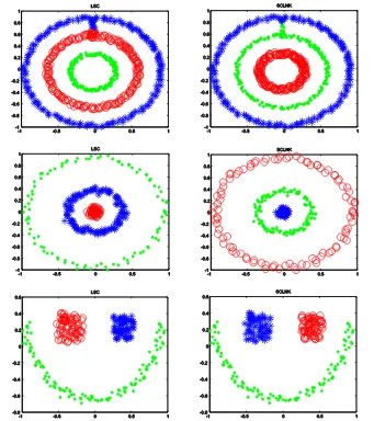
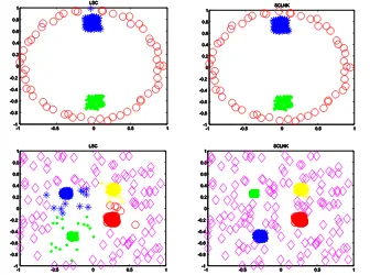
We applied the SC-LNK algorithm and LSC method to five synthetic data sets that has been mentioned in [10], [13]. The results are show in Fig. 1 and Fig. 2.

hidden in data sets which are multiscale in Fig. 2 while the SC-LNK algorithm can distinguish it after mapping to kernel space.

Fig. 1. Contrast results on Synthetic data. The left column shows the LSC algorithm

Fig. 2. Contrast results on Synthetic data. The left column shows the LSC algorithm results; The right column presents the SC-LNK clustering results. As shown above, LSC fails to find the real structure hidden in data sets while SC-LNK can distinguish.

7.2. Experiments on Real Data Sets

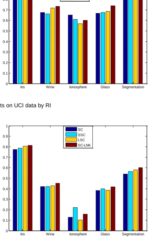
In order to extensively examine the effectiveness of the SC-LNK algorithm, we further compare the performances of our method with the other three clustering algorithms which include the SC algorithm, SSC method and the LSC algorithm. To evaluate the performance of different clustering algorithms, two different metrics are used: one is Rand index, and the other is the Normalized Mutual Information.

Evaluation metrics. Rand index (RI) is widely used to evaluate the clustering performance. A decision is considered correct if the clustering algorithm agrees with the real clustering. RI [21] is defined as

2 / ) 1 (

#  

n n

CD

where

CD

denotes the number of correct decisions. A larger RI value (

RI



[

0

,

1

]

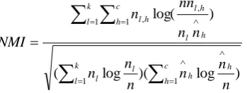
) signifies a better clustering result.

Normalized Mutual Information (NMI) is another measure for determining the quality of clusters. For two random variable

X

and

Y

, the NMI is defined as [22]:

) ( ) ( ) , ( ) , ( Y H X H Y X I Y X

NMI  ₍₁₂₎

where I(X,Y) is the mutual information between

X

and

Y

, while H(X)

and

H

(

Y

)

are the entropies of

X

and

Y

respectively. Note that ] 1 , 0 [ 

NMI and give a clustering result, the NMI is estimated as

) log )( log ( ) log( 1 1 1 1 , ,





 

        c h h h k l l l k l c h h l h l h l n n n n n n n n nn n

NMI (13)

where

n

_l denotes the number of data contained in the cluster Cl(1lk),

h

n



is the number of data belonging to the

h

-th class and

n

_l,_h denotes the

number of data which are in the intersection between the cluster

C

_l and the

h

-th class. The larger the NMI, the better the performance.

Results on uci data sets. We carry out the experiments on five data sets which come from the UCI data repository [23]. The properties of the datasets are summarized in Table 1.

Table 1. Properties of UCI Datasets

Dataset Iris Wine Ionosphere Glass Segmentation No. of instances 150 178 351 214 210

No. of attributes 4 13 34 9 19

No. of clusters 3 3 2 6 7

Iris Wine Ionosphere Glass Segmentation 0

0.1 0.2 0.3 0.4 0.5 0.6 0.7 0.8 0.9 1

SC SSC LSC SC-LNK

Fig. 3. Results on UCI data by RI

Iris Wine Ionosphere Glass Segmentation 0

0.1 0.2 0.3 0.4 0.5 0.6 0.7 0.8 0.9 1

SC SSC LSC SC-LNK

Fig. 4. Results on UCI data by NMI

in kernel space, the local relationship is maintained and different clusters are more linearly separable, thus SC-LNK can distinguish the intrinsic structure of the data more correctly.

08 358 1234 02467 0

0.2 0.4 0.6 0.8 1

SC SSC LSC SC-LNK

Fig. 5. Results on USPS data by RI

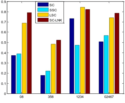
08 358 1234 02467 0

0.1 0.2 0.3 0.4 0.5 0.6 0.7 0.8 0.9

SC SSC LSC SC-LNK

Results on usps data sets. In this experiment, we consider the hand written digits from the well-known USPS database.

The digits have been normalized and centered to 16×16 gray-level images, thus the dimensionality of digit space is 256, as each sample image will be transformed to a vector as one column of the similarity graph. In the database it contains 7291 training instances and 2007 test instances.

We choose digits {0,8}, {3,5,8}, {1,2,3,4} and {0,2,4,6,7} as subsets and carry out the experiments separately. The clustering results by RI and NMI are presented in Fig. 5 and Fig. 6 separately.

According to the results in Fig. 5 and Fig. 6, we can see that the idea of linear reconstruction has a distinct advantage in the USPS data sets. The performance of LSC and SC-LNK algorithms are much better than the other two methods. Even on the challenging USPS subsets {1,2,3,4}, both of them still have improvement compared to SC and SSC though LSC is better than SC-LNK. But in most cases, the effectiveness of SC-LNK algorithm is better than LSC and the other two methods. It proves that the new similarity measure using linear reconstruction in kernel space is very helpful in detecting the real manifold of the digits.

8.

Conclusion

In this paper, we propose a novel method of constructing similarity matrix using linear reconstruction. Based on this method we introduce the concept of kernel methods and propose an efficient spectral clustering algorithm called SN-LNK. Experimental results on five synthetic data sets and two groups of the real data sets show that the proposed algorithm achieves considerable improvements over traditional spectral clustering, locality spectral clustering and self-tuning spectral clustering algorithms.

There is still much work for us to undergo further research. The similarity matrix we obtained in this paper can be extended to other clustering algorithms based on the affinity matrix. Furthermore, the selection on the number of nearest neighborhoods

k

still remains to be further studied. We will pursue these research directions in our future work.

References

1. Hagen, L., Kahng, B.: New spectral methods for ratio cut partitioning and clustering. IEEE Transactions on computer aided design, vol. 11, no. 9. (1992) 2. Shi, J., Malik, J.: Normalized cuts and image segmentation. IEEE Transactions

on pattern analysis and machine intelligence, vol. 22, no. 8, 888–905. (2000) 3. Jordan, F., Bach, F.: Learning spectral clustering. In Advances in neural

Recognition, vol. 41, no. 6, 1924–1938. (2008)

5. Wang, X., Davidson, I.: Active spectral clustering. In 2010 IEEE International Conference on Data Mining. 561–568. (2010)

6. Li, Z., Liu, J., Tang, X.: Constrained clustering via spectral regularization. In Computer Vision and Pattern Recognition. 421-428. (2009)

7. Luxbug, U.: A tutorial on spectral clustering. Statistics and Computing, vol. 17, no. 4, 395-416. (2007)

8. Roweis, S., Saul, L.: Nonlinear dimensionality reduction by locally linear embedding. Science, vol. 290, no. 5500, p. 2323. (2000)

9. Wang, F., Zhang, C.: Label propagation through linear neighborhoods. IEEE Transactions on Knowledge and Data Engineering. 55–67. (2007)

10. Gong, Y., Chen, C.: Locality Spectral Clustering. AI 2008: Advances in Artificial Intelligence. 348–354. (2008)

11. Scholkopf, B., Smola, A., Muller, K.: Kernel principal component analysis. Artificial Neural Networks-ICANN’97. 583–588. (1997)

12. Ng, A., Jordan, M., Weiss, Y.: On spectral clustering: Analysis and an algorithm. In Advances in Neural Information Processing Systems 14: Proceeding of the 2001 Conference. 849–856. (2001)

13. Zelnik-Manor, L., Perona, P.: Self-tuning spectral clustering. Advances in neural information processing systems, vol. 17, no. 1601-1608, p. 16. (2004)

14. Zhang, X., Li, J., Yu, H.: Local density adaptive similarity measurement for spectral clustering. Pattern Recognition Letters. (2010)

15. DeCoste, D.: Visualizing Mercel kernel feature spaces via kernelized locally linear embedding. In Proceedings of the Eighth International Conference on Neural Information Processing (ICONIP-01). (2001)

16. Jianbo, S., Yu, S., Shi, J.: Multiclass Spectral Clustering. In International Conference on Computer Vision. Citeseer, 313–319. (2003)

17. Meila, M., Shi, J.: A random walks view of spectral segmentation. AI and Statistics (AISTATS), vol. 2001. (2001)

18. Zhou, D., Bousquet, O., Lal, T., Weston, J., Schölkopf, B.: Learning with local and global consistency. In Advances in Neural Information Processing Systems 16: Proceedings of the 2003 Conference. 595–602. (2004)

19. Ben-Hur, A., Horn, D., Siegelmann, H., Vapnik, V.: Support vector clustering. The Journal of Machine Learning Research, vol. 2, p. 137. (2002)

20. Girolami, M.: Mercer kernel-based clustering in feature space. IEEE Transactions on Neural Networks, vol. 13, no. 3. 780–784. (2002)

21. Rand, W.: Objective criteria for the evaluation of clustering methods. Journal of the American Statistical association, 846–850. (1971)

22. Strehl, A. Ghosh, J.: Cluster ensembles--a knowledge reuse framework for combining multiple partitions. The Journal of Machine Learning Research, vol. 3, 583–617. (2003)

23. Asuncion, A., Newman, D.: UCI machine learning repository. (2007). [Online]. Available: http://www.ics.uci.edu/~mlearn/MLRepository.html

Xinyue Liu received the M.S degree in Computer Science and technology from Northeast Normal University, China, in 2006. She is currently working toward the Ph.D. degree in the School of Computer Science and Technology, Dalian University of Technology, Dalian, China. Her research interests include multimedia information retrieval, web mining and machine learning.

Xing Yong received his B.S. degree in Software Engineering from Dalian University of Technology in 2010, and currently is a master degree candidate in the same place. His major interests lie in machine learning.

Hongfei Lin received the Ph.D degree from Northeastern University, China. He is a professor in the School of Computer Science and Technology, Dalian University of Technology, Dalian, China. His professional interests lie in the broad area of information retrieval, web mining and machine learning, affective computing.