Adaptive Modulation for Finite Horizon Multicasting of Erasure-coded Data

(1)

Master of Science Thesis

Adaptive Modulation for Finite Horizon

Multicasting of Erasure-coded Data

Author:Gek Hong, Sim Master of Engineering Science

(2)

(3)

We design an adaptive modulation scheme to support opportunistic multicast schedul-ing in wireless networks. Whereas prior work optimizes capacity, we investigate the finite horizon problem where (once or repeatedly) a fixed number of packets has to be transmitted to a set of wireless receivers in the shortest amount of time – a common problem, e.g., for software updates or video multicast.

(4)

(5)

1 Introduction 1

2 Related Work 5

3 System Model 7

4 Optimization Problem 9

4.1 Dynamic programming based solution (Dyn-Prog) . . . 9

4.2 A simple two user example . . . 10

5 State-Aware Heuristics 13 5.1 Maximize minimum throughput heuristic (Max-Min) . . . 13

5.2 Weighted completion time heuristic (Weighted-CT) . . . 14

5.2.1 Choice of weights . . . 14

6 Results 17 6.1 Comparison to optimalDyn-Progsolution . . . 17

6.1.1 Homogeneous network . . . 17

6.1.2 Heterogeneous network . . . 18

6.2 Larger scenarios . . . 19

6.2.1 Impact of increasing the number of users . . . 19

6.2.2 Impact of increasing the block size . . . 22

6.3 Mutipath Rayleigh Fading networks . . . 24

6.3.1 Impact of increasing the number of users for low transmit power at BS 24 6.3.2 Impact of increasing block size for low transmit power at BS . . . . 25

6.3.3 Impact of increasing the number of user for high transmit power at BS 27 6.3.4 Impact of increasing block size for high transmit power at BS . . . 28

7 Future work 31

8 Conclusions 33

(6)

(7)

Introduction

In recent years, multicasting data to mobile users (e.g., for the purpose of video stream-ing, video conferencstream-ing, IPTV, distribution of news and alerts, or application and operating system updates) has gained in popularity and importance. As an example, the most recent mobile network architecture LTE includes the evolved Multimedia Broadcast Multicast Ser-vice (eMBMS) specifically for the purpose of distributing data and mobile TV content in a cellular network. Since the amount of such traffic in cellular networks is increasing rapidly and wireless resources are usually scarce and costly, improving the efficiency of wireless multicast is of high practical relevance.

The most common method for wireless multicasting is broadcasting. The base station (BS) transmits at some fixed low rate or the rate supported by the worst receiver to ensure that all receivers are able to receive the multicast transmission. It exploits the wireless broad-cast gain whereby a single transmission simultaneously serves all receivers. Opportunistic multicast scheduling (OMS) improves over plain broadcast by exploiting multiuser diver-sity [1]. Having the BS transmit at a rate higher than the broadcast rate to the subset of receivers that can receive at this rate improves overall throughput capacity and minimizes broadcast delay [2]. The intuition is that in an environment with variable channels, receivers that are not served in the current slot since their channel conditions are bad will be served in later slots when their conditions improve, and thus over time all receivers will eventually receive all the data. Hence, there is a tradeoff between multicast gain and multiuser diversity gain. As an extreme case, the BS may even unicast data to the receiver that supports the highest rate, serving receivers one-by-one and entirely foregoing the broadcast gain for the largest possible multiuser diversity gain. Selecting the transmission rate and thus the sub-set of receivers to multicast to is a complex problem that has been the focus of a range of OMS algorithms [3]. To simplify the scheduling problem and improve performance when multicasting data, such algortithms often use erasure codes that ensure that with high proba-bility, each packet received by a receiver is useful (unless the receiver has decoded all of the packets that exist in the system) [4], i.e., the identity of the received packets is unimportant. Fixed rate LDPC [5] or rateless LT or Raptor codes [6] are examples for such erasure codes that work well in practice and have good performance.

(8)

2 CHAPTER1. INTRODUCTION

for the case of multicasting very large files. In practice, however, multicasting data with a size on the order of hundreds to several thousands of packets much more common, partic-ularly for mobile networks. Mobile apps and operating system updates often have a size of several to several tens of MB, corresponding to thousands of packets of size 1kB. When streaming video, it is common to apply erasure coding to blocks consisting of one or several groups of pictures (GOP) [7], where a GOP usually consists of a few hundreds of packets, depending on the video rate. Since erasure coded blocks can only be decoded after they have been fully received, coding over larger blocks of video data would unecessarily increase the playout delay of the video.

In this thesis we therefore consider the finite horizon multicast problem, where a fixed amount of erasure coded data has to be delivered to a set of wireless receivers. Whenever the BS transmits a packet, the optimization algorithm has to select a suitable modulation and coding scheme (MCS). The MCS determines the amount of data transmitted per time slot and thus the data rate. At the same time, the MCS influences the packet loss probability, where more robust MCSs that transport less data are more likely to be decodable at a receiver. (We assume that the transmit power is fixed.) Our main objective is to minimize the completion time, i.e., the time needed for all receivers to successfully receive the data.

The finite horizon multicast problem is inherently more complex than the infinite hori-zon counterpart. When multicasting an infinite amount of data among a homogeneous group of receivers (i.e., with the same average channel conditions and receive rates), the optimum tradeoff between multiuser diversity and multicast gain only depends on the number of re-ceivers and their current channel conditions. In expectation, differences in the amount of data received by the different receivers will even out over time and therefore do not have to be taken into account. In contrast, the optimum decision in the finite horizon case also depends on the amount of data received thus far by each receiver (or, more accurately, on the amount of data each receiver still needs to obtain in order to decode the full block of data and thus complete). Intuitively, in case a receiver is lagging behind but many other receivers are also still for from completing, the lagging receiver may catch up by itself and jointly maximizing throughput for all these receivers may be the optimum decision. If, however, all other receivers are close to completion, optimizing the MCS (and hence the transmit rate) for the lagging receiver only may be the optimum choice to minimize overall completion time, given that all other receivers are likely to complete before the lagging receiver in any case.

The main contributions of our thesis are as follows:

•We formalize the finite horizon OMS problem and propose a dynamic programming ( Dyn-Prog) based solution, that optimally adapts the MCS to minimize thecompletion time, the time at which all receivers successfully receive the required amount of data.

• The high complexity of Dyn-Prog renders this approach unsuitable for many practical scenarios. We therefore propose a simple state-based heuristic that selects the MCS that maximizes the instantaneous throughput for the receiver with the minimum number of pack-ets which thus had the lowest throughput so far (calledMax-Min).

(9)

future states and the final state where all receivers completed, with weights based on average throughput estimates of the receivers.

• We compare the performance of our two low-complexity heuristics to the optimal Dyn-Progsolution as well as to existing approaches that greedily maximize the throughput for all receivers and a broadcasting scheme that always transmits to all receivers. We analyze sce-narios with homogeneous and heterogeneous receiver sets under a basic multi-state channel model as well as Rayleigh fading. Under Rayleigh fading, the Max-Min algorithm pro-vides a performance gain of 15% over the throughput maximization scheme and a gain of 20% over the broadcasting scheme. At a very slight increase in complexity, the Weighted-CT heuristics performs very close to the optimalDyn-Progstrategy in almost all scenarios, achieving performance gains of 25% and 40% over the throughput maximization and broad-cast scheme, respectively. For both our heuristics, the gains that can be obtained under the basic multi-state channel model are even larger.

(10)

(11)

Related Work

The idea of OMS was pioneered by Gopala and Gamal [1] who studied the tradeoff between multiuser diversity and multicast gain. They studied the performance of three dif-ferent scheduling mechanisms that adapt the transmit rate to the user with the best channel, the worst channel, and the median channel, respecively. In their follow-up paper [8], they analyzed the performance achieved by serving a fixed fraction of users. This restriction is re-laxed in [4], where the authors show that dynamic selection ratios that select more than 50% of the users can achieve higher throughput. Furthermore, a throughput maximizing scheme for erasure-coded multicast (F-OMS) is presented, where the user selection ratio depends only on the set of multicast users in the system.

The authors of [9] propose algorithms with a static selection ratio (fixed for all sions) and a dynamic selection ratio (adapted to the instantaneous channels at each transmis-sion) that maximize overall throughput. In [10], the authors extend their work of [9] from homogeneous to heterogeneous scenarios, composed of different groups of homogeneous users. A similar optimization algorithm for multicast throughput maximization in homoge-neous to heterogehomoge-neous networks is proposed in [11]. While all of these works target the infinite horizon case, in [2] the authors do consider scenarios with a finite number of mul-ticast packets. Using extreme value theory, they derive the optimal selection ratio for each transmission that minimizes completion time, i.e., the time period during which each user is selected often enough to receive the whole block of data. In contrast to our work, their optimization algorithm does not consider the state of the receivers in terms of number of packets received.

All of the above papers use a simple outage based channel model, where packet errors are deterministic. Receivers with channel conditions better than a certain threshold are guar-anteed to receive the packet and all others are guarguar-anteed to lose the packet. In real wireless systems, packet errors are much more random and depend on noise and interference. In our model, we explicitly take the relationship between the channel conditions, the chosen MCS, and the probability of error into account. Furthermore, all of the above papers – except [2] – focus on the infinite-horizon scenario and thus the performance of the proposed algorithms is sub-optimal in the finite-horizon problem we consider here.

(12)

6 CHAPTER2. RELATEDWORK

until each receiver has obtained it. The BS then multicasts the next packet in the same man-ner, and so on. The goal of the optimization algorithm is therefore to minimize the number of transmission required to multicast a single packet to all receivers, and the state of the sys-tem is the number of receivers that did not yet receive the packet. The algorithm adapts its decision to the changes in the set of users that still need to receive the packet and maximizes the throughput for those users. The approach is mainly suitable for a single homogeneous group of users, since its complexity increases exponentially with the number of user groups in heterogeneous scenarios. The method of multicasting a single packet repeatedly is less efficient than multicasting blocks of erasure coded packets as is done above.

The most basic scheme against which we compare our proposed algorithms is the broad-cast algorithm (called LCG user rate in [3]), where the transmission rate is limited by the receiver that currently has the worst channel. This scheme ensures successful transmission to all receiver at all times but may sacrifice a lot of throughput when channels are highly variable. We further compare against a scheme calledgreedythat optimizes the selection ra-tio at each transmission opportunistically based on the current channel states of all receivers so as to maximize total throughput. This mechanism has a performance that is indicative of the different selection ratio based throughput maximization algorithms above.

(13)

System Model

We model the system as a time-slotted broadcasting system with a single Base Station (BS) andN mobile users scattered within the coverage radius of the cell. Each user must receive a block of data ofBbytes and we assume that, thanks to erasure coding, each packet transmitted by the BS and received by a mobile user is useful if the user has received less thanBbytes. In case multiple blocks of data are to be transmitted in succession, the BS will start transmitting the next data block only after all the receivers fully received the current block.

A time slot is of fixed duration. Thus, the BS broadcasts the same number of symbols, which, depending on the MCS corresponds to a variable number of bytes. We assume that the BS can select one ofMMCSs, indexed bym= 1, . . . , M. The number of bytes per slot that can be transmitted using MCSmis denoted byRm.

Perfect Channel State Information (CSI) and knowledge of the number of bytes a user has successfully received is assumed to be available at the base station prior to the transmis-sion in each time slot. The users see independent channel instanceshi[k]at each time slotk,

and the discrete-time channel model for the received signal at useriis given by:

srx_i [k] =hi[k]stx[k] +ni[k], (3.1)

wheresrx

i [k]is the signal received by useriat time slotk,stx[k]is the signal broadcast from

the BS at time slotk, andni[k]is the additive white Gaussian noise term with power spectral

densityN0.

For the analysis, we assume a discrete set of Cchannel realizationsH_i for useri. The probability of useriseeing channel coefficienthi ∈ Hi in a slot is assumed to beαi(hi).

The vector of channels perceived by all users, also referred to as the channel combination, is denoted byh = {hi, i = 1. . . , N}where hi ∈ Hi. With some abuse of notation, we

denote byHthe set of all possible channel combinations, and byα(h) = QN

i=1αi(hi), the

probability of a channel combinationh ∈ H. Note that the the total number of channel combinations isH =CN.

Different from the prior work discussed in Section 2, we do not assume deterministic channel outage but use the probability of error (PER) for a given channel and MCS from [13] in order to model the erasure probability. Therefore, for a channel instancehi∈ Hi, the PER

for useriunder MCSmis represented bypm

i (hi), and the probability of success is given by

(14)

8 CHAPTER3. SYSTEMMODEL

In this thesis, we use the following terms:

(1) Astrategygspecifies the MCSg(h)for each channel combinationh ∈ H. Hence, the total number of strategies isS =MH. We denote byG, the set of all possible strategies. (2)

The stateconsists of the vector of the number of bytes received by each useridenoted by

x={xi, i= 1, . . . , N}. The state spaceX consists of all states where the number of bytes

received by all users is positive and less than or equal toB. Theinitial statewhere none of the users have any information is x0 _{and the end state where all the users have received} _B

bytes is denoted byxB.1

(3) Apolicyµmaps any given statex∈ X to the strategygµxto be used in that state.

(4) Theexpected completion timeDµ(x)is the mean time required to get from statexto the

end statexBunder policyµ.

1

(15)

Optimization Problem

In this section, we consider the case of memoryless channels and formulate the problem as a stochastic shortest path problem [14] with cost per stage equal to 1 (time needed per slot is fixed, τ = 1) and no terminal cost. We assume that the probability of successfully receiving a packet is non-zero for every combination of modulation scheme and channel condition, though it might be extremely low for some combinations.

4.1 Dynamic programming based solution (

Dyn-Prog

)

LetE ={e| |e|=N, ei∈ {0,1}}be the set of all vectors of sizeN whose components

take values 0 or 1. The transition probability from statex∈ X to statey ∈ X when MCS

mis used under channel combinationhis given by:

ρm_h(x,y) = X

min(x+Rme,B)=y e∈E

N

Y

i=1

pm_i (hi)eiqim(hi)1−ei

!

, (4.1)

where the above minimization is defined element-wise. Note that in the case of every user experiencing an erasure, the state remains unchanged.

The state space is finite, and there clearly exists a finite integer K such that there is a positive probability of terminating afterKsteps irrespective of the policy. Thus, the optimal policyµ∗satisfies Bellman’s equations at every statex:

Dµ∗(x) = min

g∈G



1 + X

h∈H

α(h)X

y∈X

ρg_h(h)(x,y)Dµ∗(y) 

, (4.2)

and the optimal strategy at statex

gµ∗(x) = argmin

g∈G



 X

h∈H

α(h)X

y∈X

ρg_h(h)(x,y)Dµ∗(y) 

. (4.3)

(16)

10 CHAPTER4. OPTIMIZATIONPROBLEM

Starting from the end statexB, we use Bellmann’s equation Eq. 4.2 to determine the com-pletion times of the states that only depend on the end state (for which the comcom-pletion time is known to be0). We then proceed in the same manner to determine the expected completion times of states that only depend on states for which the completion time is already known, until the completion times for all states are computed. This process also yields the optimum policies from Eq. 4.3.

4.2 A simple two user example

Consider a scenario with two users (N = 2), with identically distributed channels. Let

H1 = H2 = {L, H}, and H = {HH, HL, LH, LL}, where L andH denote channels

with low and high channel quality, respectively. The base station can choose one of three modulation schemes in each slot. The probability of packet error when MCS mis used is denoted bypm₍_L₎_and_pm₍_H₎_{for both users under the low and high channel respectively. A}

strategy is defined by specifying the modulation scheme to be used for each vector channel inH.

In this example, Bellman’s equation at state{x1, x2}is:

Dµ∗({x₁, x₂}) = 1 + min

g∈G

X

h∈H

α(h)

pg(h)(h1)pg(h)(h2)Dµ∗({x₁, x₂})

+pg(h)(h1)qg(h)(h2)Dµ∗({x₁,min(x₂+R_g₍_h₎, B)})

+qg(h)(h1)pg(h)(h2)Dµ∗({min(x₁+R_g₍_h₎, B), x₂)})

+qg(h)(h1)qg(h)(h2)Dµ∗({min(x₁+R_g₍_h₎, B),

min(x2+Rg(h), B)})

We evaluate the optimal policy in a scenario where theH andLchannels for the users areH1=H2={5dB,28dB}. The probability ofLandHareα1(L) =α2(L) = 0.75and

α1(H) =α2(H) = 0.25. We choose such a highly variable channel, since it makes it easier

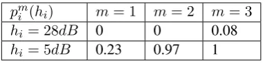
to demonstrate the decision tradeoffs that the algorithm makes in the different regions of the state space. The probability of each channel combination in Hcan be easily obtained by multiplying the respective channel probabilities. For simplicity, we only useM = 3MCSs with normalized rates ofRm=1 = 1,Rm=2= 4andRm=3= 9and the PER for each MCSs

and channel instant is listed in Table 4.1.

Table 4.1: PER for different MCS and SNR value pair

pm_i (hi) m= 1 m= 2 m= 3

hi = 28dB 0 0 0.08

hi = 5dB 0.23 0.97 1

(17)

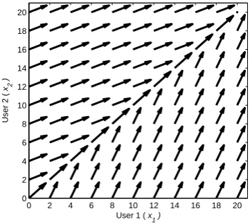
correspond-0 2 4 6 8 10 12 14 16 18 20 0 2 4 6 8 10 12 14 16 18

User 1 ( x 1 )

User 2 (

x2

)

Figure 4.1: Optimal policy with the dynamic programming algorithm (Dyn-Prog)

0 2 4 6 8 10 12 14 16 18 20 0 2 4 6 8 10 12 14 16 18 20

User 1 ( x₁ )

User 2 (

x2

)

Figure 4.2: Max-Min Algorithm

0 2 4 6 8 10 12 14 16 18 20 0 2 4 6 8 10 12 14 16 18 20

User 1 ( x 1 )

User 2 (

x2

)

Figure 4.3: Weighted-CT algorithm

ing policy.1 We set the (normalized) block size B = 20. At the initial statex0 = {0,0}

the optimal policy isg(h) ={1,3,3,3}, i.e., MCSm= 1is used for channel combination

LLand MCSm = 3is used for channel combinationsLH,HL, andHH. This particular policy is a greedy policy which gives the maximum throughput to both users. This pol-icy is also used in almost all states up to x = {14,14}. Closer to the borders of the state space, the policy changes from greedy to more and more favoring the user that is lagging behind. This accounts for the fact that the leading user is likely to finish before the trailing user even if MCS decisions are optimized for the trailing user and aims to prevent the loss of multiuser diversity caused by a user finishing early. For {14 < x1 ≤ 16, x2 < 14}

and {x1 < 14,14 < x2 ≤ 16}, the predominant policies are g(h) = {1,3,2,3} and

(18)

pre-12 CHAPTER4. OPTIMIZATIONPROBLEM

vent the trailing user from falling further behind. Even closer to the borders the policies are

g(h) ={1,3,1,3}andg(h) ={1,1,3,3}, even further trading off overall throughput for a higher packet reception probability for the trailing user. When both users received a similar number of bytes and are close to the end statexB, the algorithm also chooses a more con-servative MCS indicated by a shorter arrow length to avoid overshooting (i.e., unnecessarily delivering more thanBbytes to both users).

(19)

State-Aware Heuristics

Due to the high complexity of theDyn-Progalgorithm introduced in the previous sec-trion, we propose two low-complexity heuristics that mimic the characteristic ofDyn-Prog

algorithm.

5.1 Maximize minimum throughput heuristic (

Max-Min

)

This heuristic is based only on the current state (the number of bytes that each user has successfully received), and the current channel conditions. At each slot, the user with the least number of received bytes is identified as the worst user who is most likely to require the highest number of slots to receive all data. Note that this is indeed the case when the users are homogeneous and perceive identical channel distributions. In the case of heterogeneous users, those users that perceive channel conditions that are worse (on average) are highly likely to also be the trailing users and thus most likely to finish last. The algorithm uses in each slot the MCS that maximizes the throughput for the trailing user. If both users have the same number of bytes, the algorithm greedily maximizes sum throughput for both.

Figure 4.2 depicts the average drift resulting from such a policy in a scenario with the same parameter setting as explained in Section for homogeneous users. There are two pre-dominant strategies that are used for all states off the diagonal. As Max-Min sacrifices overall throughput in favor of the trailing user as soon as a user falls behind, the resulting strategies areg(h) = {1,3,1,3}andg(h) ={1,1,3,3}. On the diagonal,Max-Min’s sum throughput maximization leads to the same strategy as in theDyn-Progsolution, except for the last state before finising. Since in contrast to theDyn-Prog,Max-Mindoes not explicitly take expected completion time into account, it does not switch to more conservative sym-metric strategies ofg(h) ={1,2,2,2}andg(h) ={1,1,1,1}, respectively, that deliver the required number of bytes to finish with a lower packet loss probability compared to using the highest MCSm= 3(which would result in delivering more bytes than necessary to the receivers).

(20)

14 CHAPTER5. STATE-AWAREHEURISTICS

5.2 Weighted completion time heuristic (

Weighted-CT

)

In many cases, favoring the trailing user is overly conservative. In particular, when the number of pending bytes is large for all users and the relative lag is small, the probability that the currently trailing user finishes last is small. We now present a heuristic that more closely models the decisions taken by theDyn-Progalgorithm to achieve a better tradeoff between instantaneous sum throughput and balancing the number of bytes pending for different users. At slotk, with statexand channelh, we evaluate the average drift and determine the expected next state,ym, conditioned on using modulation schememas:

y_im =xi+qmi (hi)Rm, i= 1, . . . , N (5.1)

We then estimate the additional time required, on average, for all users to receiveBbytes rel-ative to other states. Since computing the average remaining time under the optimal policy is computationally intensive, we use a weighted Euclidean distance measure in order to char-acterize the difference in completion times from different states. The metric τyassociated

with stateyis:

τy=

v u u t N X i=1

(B−yi)

wi

2

(5.2)

Here, the weights reflect the average channel conditions perceived by each user, with a user that perceives poor channels on average associated with a lower weight. The modulation scheme chosen at slotkism∗ = arg minmτym.

5.2.1 Choice of weights

We choose weightswi that are proportional to the average throughput achieved by the

user under a hypothetical policy that chooses the MCS uniformly at random, i.e.,

wi =

X

h∈H

M

X

m=1

α(h)qm_i (hi)Rm.

As the actual choice of MCS depends on the state as well as the channels of the other users and cannot be determined in advance (sort of using the optimum decisions given by the Dyn-Prog), this hypothetical policy is a very simple method to capture the relative throughput differences among the users.

In practical scenarios, the channel distribution of individual users may not be known in advance. Further, the channel statistics of a mobile user may change over time, albeit on time scales that are slow with respect to average completion times. In such settings, we use exponentially weighted averaging in order to track the user weights. The estimated weight of useriat slotk,wˆi[k], when the perceived channel ishis given by:

ˆ

wi[k] = (1−β) ˆwi[k−1] +β M

X

m=1

q_im(hi)Rm, (5.3)

(21)

(22)

(23)

Results

In this section, we evaluate and study the performance of our proposed algorithms in homogeneous and heterogeneous scenarios and compared them to the existing broadcast

andgreedyschemes. For small scenarios (N = 2) we also compare our results to the optimal

Dyn-Progsolution. First of all, we study the performance in a simple scenario, i.e.,N = 2

users,C = 2channel instances to build an intuition towards more complicated scenarios. Later, we study the impact of block size B as well as number of user N and finally, we analyze performance under multipath Rayleigh fading channels with path loss model from COST207 [15] and Winner Model II [16], respectively.

In all of the simulations, we consider 3 modulation types BPSK, QPSK and QAM with channel codes code with code rates 1/2, 2/3 and3/4, resulting in seven different MCS. These correspond to rates of 6, 12, 24, 36, 48, and 54 Mbps. The corresponding PER with respect to the instantaneous channel quality for each MCS is obtained from [13]. For the performance metric we use average throughput which we compute as follows:

η = B

D M bps (6.1)

whereηis the average throughput,B is the normalized block size andDis the completion time. Here, we consider normal MTU sized packets of1500Bytes. In this Chapter, block size and normalized block size are use interchangeably but both of them represent the size normalized block size corresponding to the greatest common divisor of the MCS rates.

6.1 Comparison to optimal

Dyn-Prog

solution

In this section, we first analyse the performance of the different algorithms in a simple

N = 2with C = 2channel instances and M = 7modulations scenarios. This simple scenario allows us to obtain the optimumDyn-Progsolution. We study both homogeneous and heterogeneous user scenarios.

6.1.1 Homogeneous network

(24)

18 CHAPTER6. RESULTS

result of increasing the channel variability δ of the users. Channel variabilityδ is the dif-ference between the H and L channel of each user. For instance, in this case the lowest channel variability isδ = 4(H = 11dB andL= 6.7dB) and the highest channel variability isδ = 20.8(H = 20dB and L= 0.2dB). Each channel variability pair is chosen such that the average throughput for each pair remains fixed, which facilitates the comparison of the results. In addition, we also fix the stationary channel probability for high (α(H) = 0.25) and low (α(L) = 0.75) channel. The normalized block size isB = 200.

Figure 6.1 depicts the average throughput of each scheme as the channel variabilityδ

increases. As expected,greedyscheme performs well since the users have the same average channel conditions. Greedyscheme optimizes the throughput therefore, in this scenario it is able to equally serves both users. TheWeighted-CTscheme similarly optimizes throughput and simultaneously serves all the user in a fair manner while ensuring low delay. On the other hand, theMax-minscheme is overly conservative towards the trailing user as it tries to balance the users even if the trailing user is only lagging by a small number of bits. As the

broadcastscheme is limited by the user with the worst channel, it is transmitting at the

low-est MCS most of the time. While it is expected that the performance of bothMax-minand

broadcastdecreases since theLchannel degrades as the variability increases, it is interesting

that the performance ofgreedy,Weighted-CTandDyn-Progfirst decreases but then slightly improve later. This is because of the MCS chosen which gives the highest possible through-put. For instance, whenδ = 4dB, the throughput optimization choices areRm = {4,2,2

and 2} for channel combination Has mentioned in Chapter 6.1, but the throughput opti-mization choice atδ = 10dB isRm ={4,4,4and2}. It can easily be calculated that the

normalized throughput atδ = 10dBis lower than that atδ = 4dB. Here, theWeighted-CT

scheme behaves like the greedyscheme in the sense that it tries to give as much as possi-ble to both users. Since the average channels of the users are the same, the weights wfor both the users are the same as well. Another unusual performance forMax-Minis when it downperfroms all the schemes includingbroadcastbecause giving at higher rate while the trailer hasHchannel is not optimal (see per slot throughput comparison in Figure 6.2(a)) as compared to giving to both users as an average rate. On the contrary,broadcastscheme per-forms worse thanMax-minbecause the bad channel quality became worst whenδincreases and it is unreasonable to serve the worst channel user while sacrificing a lot of throughput. Figure 6.2(b) shows the average achievable sum throughput forbroadcastscheme is consis-tently lower than the rest because it ignore the opportunity of sending at a much higher rate that results in higher sum throughput.

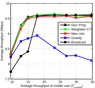
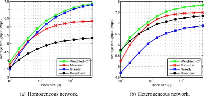
6.1.2 Heterogeneous network

In the heterogeneous channel model, we assume that one user does not move (fixed user) while the other user is moving towards BS (mobile user) with an initial distance equivalent to that of the fixed user. In another word, the mobile user have an increment in itsH andL

channel’s SNR value. The first extreme in the graphs is when both users are homogeneous and having high channelHf ixed =Hmobile = 15dB and low channelLf ixed =Lmobile =

5dB. On the other extreme, the fix user’s channel instances isHf ixed = 15dBandLf ixed =

5dB while the channel instances for the mobile user is Hmobile = 29dB and Lmobile =

(25)

α(L) = 0.75.

In Figure 6.1(a), the performance ofbroadcastscheme is bad in homogeneous scenario, it also applies when the heterogeneity of the users is not high. As the heterogeneity increases where the average throughput of the mobile user increases,broadcastandMax-minscheme which always favour the worst or trailing users have advantage overgreedyscheme. Since the parameters setting in forδ= 10dBFigure 6.1(a) and first point in Figure 6.1(b) is simi-lar, it gives the same average throughput. As other scheme gradually increase in their perfor-mance,greedy’sthroughput also initially improves however it degrades as the heterogeneity increase because the rates used for transmitting a packet is higher andgreedytends to give to the mobile user when its channel improves and leaves the fixed user with a higher backlog which cost greedy with a higher completion time. However, Weighted-CT cares to serve both user under all circumstances, here it behaves likeMax-minas it assigns lower weight to fixed user than mobile user. In addition, we include the per timeslot throughput perfor-mance for low heterogeneity (see Figure 6.2(c)) and high heterogeneity (see Figure 6.2(d)) networks. In these figures, the average sum throughput is computed based on the chosen MCS and channel combination at each time slot. For the purpose of clear comparison be-tween scheme, we take a sample once every5 time slots. In Figure 6.2(a), we observe a clear two level of average sum throughput. For number of userN = 2, on average the first user receive the complete data within120slots and the second user complete in an approx-imate of150slots for all the schemes. While Figure 6.2(a) and Figure 6.2(b) only show a two levels of sum average throughput, Figure 6.2(c) and Figure 6.2(d) show more than two levels of sum average throughput. In heterogeneous network, users are distinct, on average, the mobile (good channel quality) user will finish much quicker than the fixed (bad chan-nel quality) user. There exist a clear second and third levels in Figure 6.2(d) especially for

greedyscheme because the fixed user remains in the system for some times before it receives

all the desired information. As we only have two types of user (i.e., mobile and fixed), we cobserve thatgreedyhas a much higher throughput than the other scheme because it greed-ily serves the good users (i.e., users with better channel quality) while ignoring the bad user and when all the good users received all the intended packets, it has a longer time slots with lower throughput because the users left are the bad users with high and low channel of15dB

and5dB, respectively. We also perform simulations for these scenarios by using a larger block size B = 5000 and it results in the same performance for both homogeneous and heterogeneous scenarios.

6.2 Larger scenarios

In this section, we present the simulation results for the scheme in two different higher complexity settings (i.e., impact of increasing the number of users in the system and impact of increasing the block sizeB and study the performance.

6.2.1 Impact of increasing the number of users

(26)

6 8 10 12 14 16 18 5.5 6 6.5 7 7.5 8 8.5 9 9.5

Channel variability δ (dB)

Average throughput (Mbps) Dyn−Prog

Weighted−CT Max−min Greedy Broadcast

(a) Homogeneous network with increasing channel variabilityδ(Point 4 corresponds to Point 1 in Het-erogenous graph Figure 6.1(b)).

10 15 20 25 30 35

7.5 8 8.5 9 9.5 10

Average throughput of mobile user (T_mobile)

Average throughput (Mbps)

Dyn−Prog Weighted−CT Max−min Greedy Broadcast

(b) Heterogeneous network with increasing hetero-geneity.

Figure 6.1:2-user scenario with block sizeB = 200

for theHandLchannel as in Chapter 6.1. For the homogeneous scenario, the correspond-ingH andLchannels are 19dB and2.5dB, respectively. In the heterogeneous user case, the correspondingH andLfor fixed and mobile users areHf ixed = 15dB, Lf ixed = 5dB

andHmobile = 27dB, Lmobile = 17dB, respectively. The number of user increases

expo-nentially fromN = 2toN = 64.

Figure 6.3 shows that the average throughput for all the schemes decreases as the number of user increases because it is more difficult to find decisions that jointly optimize perfor-mance for a larger number of users. At the same time, since completion time is determined by the slowest user, as the number of user increases, it becomes more probable that some users see a high number of bad channels and lag far behind. In the homogeneous scheme (see Figure 6.3(a)) it is expected thatbroadcastscheme performs the worst in this scenario because it tends to be very conservative and always transmit at the lowest rate at least90%

of the time.Max-minhowever, performs better although it tries to keep both users as close as possible regardless of the relative difference in the number of bits obtained. As explained in the Chapter 6.1, homogeneous user distribution gives advantage to greedyscheme because it tries to give to all users at the highest possible throughput which also explains the good performance ofWeighted-CT.

In Figure 6.3(b), we see the same pattern where the average throughput decreases with an increasing number of user for the same reasons as above. It is interesting to note that the

broadcastscheme performs better thanMax-minfor a higher number of users. This is due

to the fact that optimizing for the trailing user is similar to broadcasting to all users. Max-minloses throughput when it favors the trailing user, without taking into account that this user may have a better channel later. When the channel of the trailing user becomes better,

Max-minwill transmits at a higher rate causing high PER for low channel user who might

(27)

0 50 100 150 0 0.5 1 1.5 2 2.5 3

Number of time slots

Average sum throughput

Weighted−CT Broadcast Greedy Max−min

(a) δ= 4.3dB,H= 11dB,L= 6.7dB

0 50 100 150 200 250

0 0.5 1 1.5 2 2.5 3

(b)δ= 14.8dB,H= 18dB,L= 3.2dB

0 50 100 150 200

0 0.5 1 1.5 2 2.5 3 3.5

(c) Average throughput =12.7,H = 17dB,L= 7dB

0 50 100 150 200

0 1 2 3 4 5 6

(d) Average throughput =29.9,H = 27dB, L = 17dB

Figure 6.2: Throughput comparison between schemes in homogeneous (Figure 6.2(a) and Figure 6.2(b)) and heterogeneous scenario (Figure 6.2(c) and Figure 6.2(d))

their different weights. It is also interesting to note that, the performance of broadcast

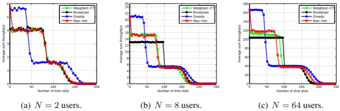
scheme is unusual when compared to other schemes as the number of user increases. We compare the per-slot sum throughput for different number of user in Figure 6.4 and notice that performance in Figure 6.4(b), as compared to that in Figure 6.4(a) and Figure 6.4(c), the sum throughput difference betweenWeighted-CT andbroadcastis greater in Figure 6.4(b).

Broadcast throughput is bounded by the worst channel whileWeighted-CT and Max-min

have better chance to transmit at higher rate as the number of user increases while the choice is limited when the number of user is as small asN = 2. Therefore for case withN = 2,

Weighted-CT andMax-minperform similar tobroadcast. By equally serving the fixed and

mobile users asN increases, Weighted-CT obtains lower sum throughput as compared to

Max-min at the beginning of the transmission but it reduces the time taken for the fixed

(28)

22 CHAPTER6. RESULTS 101 4.5 5 5.5 6 6.5 7 7.5 8 8.5

Number of user (N)

(a) Homogeneous network.

101 5.5 6 6.5 7 7.5 8 8.5 9 9.5 10

(b) Heterogeneous network,

Figure 6.3: Fixed block size ofB = 200with increase number of user

0 50 100 150 200

0 1 2 3 4 5 6

(a)N = 2users.

0 50 100 150 200 250

0 2 4 6 8 10 12 14 16 18 20 22 24 25

(b)N = 8users.

0 50 100 150 200 250

0 20 40 60 80 100 120 140 160 180

(c) N= 64users.

Figure 6.4: Throughput comparison between schemes for differentN in heterogeneous net-work.

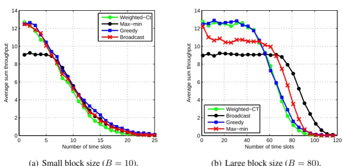
6.2.2 Impact of increasing the block size

We use similar parameters as in Chapter 6.2.1 except that here we set the number of user toN = 10and investigate the performance as the block size increases exponentially from

B = 10toB = 5120. Different from the performance in Figure 6.3, throughput increases as the block size increases (see Figure 6.5). At smaller block size, it is easier for the good user to finish but this leaves the bad user in the system and it will take as much time as the worst user to finish. With the probability of being in bad channel3times greater than good channel, it is very likely to encounter bad channel within the next time slots. However, when the block size increases, users will stay in the system for a longer time. As we compare the drop off time in Figure 6.7(a) and Figure 6.7(b), the fraction of drop off time with respect to the total completion time is larger (approximately 85%) for small block sizeB = 10, and smaller (approximately 60%) for a larger block sizeB = 80. In another word, the longer is the time all the user stay in the system together, the more likely will the time to broadcast to all user be shorter. From all the previous results, we already know that bothbroadcastand

Max-mindownperforms the rest in homogeneous scenario andgreedyis expected to perform

(29)

the users who are currently inL = 5dB channel to obtain any new data byte and cost it a higher completion time (see Figure 6.7(a)).

101 102 103

3 3.5 4 4.5 5 5.5 6 6.5 7 7.5

Block size (B)

101 102 103

4.5 5 5.5 6 6.5 7 7.5 8

Block size (B)

(b) Heterogeneous network.

Figure 6.5: Fixed10users scenario with increase number of packets

In the heterogeneous users scenario, broadcast performs as good asWeighted-CT be-cause when the number of packet is as small as B = 10 and the highest normalized rate that we have is9, it is only important to serve the users in the bad channel especially for the case of heterogeneous users when there exists one clear bad user (fixed user). This is also the reason for whichgreedyscheme underperforms the rest of the schemes as it only oppor-tunistically optimize for the mobile (good) users. It can give a much higher instantaneous throughput than favoring the fixed (bad) user.Max-minis expected to outperformbroadcast

scheme as block size increases becausebroadcastignores the opportunity of sending at high rate which caused the lost in throughput.

0 5 10 15 20 25

0 2 4 6 8 10 12 14

Weighted−Ct Max−min Greedy Broadcast

(a) Small block size (B= 20).

0 20 40 60 80 100 120 0 2 4 6 8 10 12 14

(b) Large block size (B= 80).

(30)

0 5 10 15 20 25

0 2 4 6 8 10 12 14

Weighted−Ct Max−min Greedy Broadcast

(a) Small block size (B= 10).

0 20 40 60 80 100 120 0 2 4 6 8 10 12 14

(b) Large block size (B= 80).

Figure 6.7: Average sum throughput per time-slot for different block size in homogeneous network.

6.3 Mutipath Rayleigh Fading networks

All previously shown results are the baseline for the performance simulated in this sec-tion. In the following, we include the actual multipath model (from COST207 model [15]) and path loss model (from Winner Model II [16]) as our channel model. In the subsequent, we evaluate the performance in both homogeneous and heterogeneous user’s network for different block sizeB and number of userN scenarios with different transmit power from the BS. In the homogeneous scenario, we place the users at an equidistant from the base station while in the heterogeneous scenario, we place them at a different distance from the base station. The multipath Rayleigh channel distribution of the users are independent and identically distributed (non i.i.d) in homogeneous scenario and non-i.i.d in heterogeneous scenario. The lowest transmit power is set such that the edge user is still able to receive the transmitted data at its average channel. We also analyse the performance of the effect of having low and high power transmitter. For the different transmission powers (low & high), we show the results for the impact of exponentially increasing block size with fixed number of user. In addition, the performance is also evaluated for exponentially increase in number of user with fixed block size.

(31)

Homogeneous network. In Figure 6.8(a), all the schemes tend to perform the same when N = 2which is in contrast to that in Figure 6.3(a). This is because of the unlikeli-hood of staying in only two channel instantaneous (i.e., the simple case in Chapter 6.1 and Chapter 6.2 withC= 2) due to the Rayleigh distributed channel. In addition, as the number of user in the system is small, the users are not fully homogeneous because the transmission period is too short for the user to see the average channel. Later, the performance converges to what we expected which is comparable to that in the simple case (see Figure 6.3(a)) be-cause the homogeneity among users is achievable as the number of user increases, i.e., the transmission period needed to serves higherN is much longer. Overall, each scheme still behaves in the same way (i.e.,broadcastscheme still performs the worst among all the other scheme).

Heterogeneous network. In the heterogeneous scenario, we observe from Figure 6.8(b) that the greedy scheme performs as expected. However the broadcast scheme performs better than the rest of the schemes when the number of user is small. When there are only

N = 2users in the system, it is clear in heterogeneous case that the users are having very distinct channel instances (i.e., high SNR for one and low for the other) and the optimal scheme is a scheme that always gives to the user who constantly has the lower channel SNR among the two. Therefore, in this situation,Max-minandbroadcastschemes perform the best. The channel variationδbetweenHandLchannel is alwaysδ= 10dBin Chapter 6.1.2 and the lowest channel SNR is5dB. In contrast,δ in multipath Rayleigh fading from one channel instant to another can be very small (e.g. δ = 0.1dB) and the lowest channel SNR in deep fades can be below0dB. Therefore, the smooth transition between the highest and lowest channel SNR gives throughput avantage toMax-minoverbroadcastscheme for

the trailer (trailing user) does not always has the lowest channel SNR. Therefore,

Max-minhas high chance of transmitting at a higher rate as compared tobroadcastscheme. In addition, the deep fade caused by multipath Rayleigh fading induced a high throughput lost

tobroadcastscheme over all the other schemes in a system with higher number of user (e.g.

N = 64) for transmitting at a lowest possible rate. In contrast, the traileris not always the user with the worst channel inMax-minscheme. Therefore deep fade channel does not greatly affect the throughput performance ofMax-min.

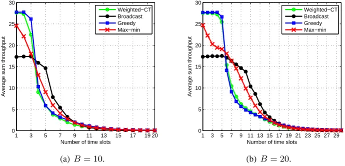
6.3.2 Impact of increasing block size for low transmit power at BS

Here, we fix the number of user toN = 10and observe the impact of increasing block size fromB = 10toB = 5120towards the average throughput in both homogeneous and heterogeneous network scenarios for which BS is transmitting at low power.

Homogeneous network. As the block size increases, we observe in Figure 6.10(a) that the performance curve is very similar to that in the simple scenario case (see Figure 6.5(a)). However, the performance ofbroadcastscheme is better than all the other schemes including our proposed schemes. First of all, it only consumes about 12 (see Figure 6.9(a)) and19

(32)

26 CHAPTER6. RESULTS 101 4 6 8 10 12 14 16

Weighted−CT Max−Min Greedy Broadcast

101 4 5 6 7 8 9 10 11 12 13

(b) Heterogeneous network

Figure 6.8: Increasing the number of user in multipath network with low transmit power at BS.

schemes because the most important user is the one user who is having the worst channel instances within the entire transmission slots. As the block size increases, the users achieve almost similar average channel SNR (i.e., users are close or almost homogeneous) within a longer transmission slots, therefore, the performance in Figure 6.10(a) is now comparable to that obtained in Figure 6.5(a).

1 3 5 7 9 11 13 15 17 19 20 0 5 10 15 20 25 30

(a) B= 10.

1 3 5 7 9 11 13 15 17 19 21 23 25 27 29 0 5 10 15 20 25 30

(b)B= 20.

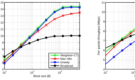
Figure 6.9: Per time slot average sum throughput performance in homogeneous network. Heterogeneous network. Figure 6.10(b) depicts the impact of increasing block size towards the performance of each scheme. For the same reason explained above, the existing of a clear worse user causedbroadcastscheme to outperform the rest of the scheme when the block size is very small. Weighted-CT,Max-minandgreedyschemes perform as expected where greedyscheme performs the worst among other scheme in heterogeneous network.

(33)

101 102 103 5 6 7 8 9 10 11 12 13 14 15

Block size (B)

(a) Homogeneous multipath network.

101 102 103

4 5 6 7 8 9 10 11

Block size (B)

Per−packet throughput (Mbps) _{Weighted−CT}

Max−Min Greedy Broadcast

(b) Heterogeneous multipath network.

Figure 6.10: Increasing the block size (B) in multipath rayleigh fading network with low transmit power at BS.

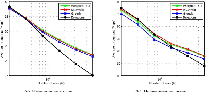
6.3.3 Impact of increasing the number of user for high transmit power at BS Different from Chapter 6.3.1, here we consider a scenario where the transmit power of the BS is increased. Similarly, we can also place the users closer to the BS as compared to that in Chapter 6.3.1 instead of increasing the transmit power at the BS. Like the setting in Chapter 6.3.1, we fix the normalized block size toB = 200and observe the impact of increasing number of user fromN = 2toN = 64towards the average throughput in both homogeneous and heterogeneous network scenarios.

Homogeneous network. Figure 6.11(a) shows that the overall performance between schemes is very similar to that in Figure 6.8(a) when users are homogeneous. It is interesting to note thatgreedyscheme downperformsMax-minscheme, conflicting the result obtained in Figure 6.11(a). At a certain channel instantaneous, there will be one or more users having channel SNR much higher than the others (channel SNR ranges between15dB and30dB) which means transmitting at a much higher rate gives a very high throughput but it burdens the bad channel users.Greedyscheme is suboptimal because the maximum average number of time slots needed is less than 80for broadcastscheme (i.e., other schemes need much lower number of time slots). This means that, the users does not see enough channels to obtain the same average channel among users. It is clear that, under this situation,Max-min

scheme that optimizes for the trailer performs very close toWeighted-CT which also pays attention to the trailer. As forbroadcastscheme, it still performs badly although the bad user does not see deep fade channel as low as that in the low transmit power at BS case (e.g. The average SNR is between20dBand27dBbut the deep fade can go from15dBto as low as

0dB). Weighted-CT performs the best among all other schemes because it tries to transmit

at the highest possible rate without causing the trailer to have a high backlog.

(34)

the transmit power is high. When users are heterogeneous, giving more data to the good channel user that results in a slightly shorter average completion time D is the optimal strategy forWeighted-CTbecause the gain from transmitting at high rate for good user (with high channel SNR) is higher than the lost by the low channel SNR’s user. This has leads to higher throughput at the earlier time slots and introduces some backlog for the low channel user. Therefore, in this scenario (heterogeneous network withB = 200)Max-minperforms very well. As mentioned in Chapter 6.3.1, short transmission time gives opportunity to

broadcastandMax-minto perform better than the other scheme especially when the number

of user low and only requires an average of 30 to40 time slots to complete the multicast transmission. 101 15 20 25 30 35 40

(a) Homogeneous users

101 10 15 20 25 30 35 40

(b) Heterogeneous users

Figure 6.11: Increasing the number of user in high power transmitter network

6.3.4 Impact of increasing block size for high transmit power at BS

Here, we fix the number of userN = 10 and observe the impact of increasing block size fromB = 10toB = 5120towards the average throughput in both homogeneous and heterogeneous network scenarios for which BS is transmitting at high power.

(35)

throughput as it tries to serve all the users with the least transmission rate limited by the worst channel at a time slot. The performance ofMax-minlies betweenWeighted-CT and

broadcastbecause it not only serves the trailer but it also obtains chances to serve at a high

rate when the trailer has a good channel (a chance to achieve higher throughput).

101 102 103

10 15 20 25 30 35 40

Block size (B)

101 102 103

12 14 16 18 20 22 24 26 28 30 32

Block size (B)

(b) Heterogeneous users

Figure 6.12: Increasing the number of packets in in high power transmitter network Heterogeneous network. Figure 6.12(b) also inherited the same performance of broad-cast scheme as in Figure 6.10 and it is as expected. It is also clear thatMax-minperforms close toWeighted-CTin heterogeneous users scenario. One major difference between trans-mitting at high power (see Figure 6.12(b)) and low power (see Figure 6.10(b)) in heteroge-neous network is the performance ofgreedyscheme at large block size. With high power,

greedy performs much closer toWeithted-CT because the users are having better channel

(36)

(37)

Future work

In this thesis, our main objective is to derive an optimal solution with two other heuris-tics (Max-minandWeighted-CT) that minimize the total time required for all the multicast users to successfully receive a common set of data which is based on assumptions such as perfect channel and state knowledge, fixed number of users for the duration of transmitting the common set of data bytes to all multicast users, no constraint on energy and etc. In addition, we only consider a single hop multicast from the BS to the end user. An actual implementation however should not make the aforementioned assumptions. Following is the list of our major focuses of research in the near future:

1. Eliminating the assumption of perfect channel and state knowledge at the BS by taking into consideration the feedback from the end user. The channel quality is estimated based on the received signal strength of the feedback packet from the end user while the state knowledge is directly provided by the end user. Acquiring the feedback from the end user at each time slot is a burden to the network. Therefore, we aim to design a model whereby feedback is only acquired from the user whose channel quality is higher than a certain threshold to avoid serving the user when its channel quality is too low. In addition, this allow the reduction on the feedback load.

2. Joint network coding and cooperative transmission between users in a network coding based sensor network can greatly improve the throughput performance of our scheme. We intend to extend our single hop model to a cooperative network coding model so that a user with more data can perform coding to the received data and forward it by broadcasting it to the users in the same multicast group. We will use ourWeighted-CT

algorithm at the relay station for it to choose the optimal MCS once the end nodes’ or relay nodes’ channel and state are known.

(38)

(39)

Conclusions

In this thesis we investigated the finite horizon opportunistic multicast scheduling prob-lem, where a wireless base station has to transmit a fixed amount of erasure coded data to a set of receivers. We designed an algorithm based on dynamic programming that, to the best of our knowledge, is the first to explicitly take into account the system state in terms of received amount of data at each receiver for the selection of the optimum modulation and coding scheme. In addition to the well known tradeoff between broadcast gain and multiuser diversity gain that is inherent to opportunistic multicast scheduling, the finite horizon nature of our problem introduces an interesting further tradeoff, namely that of equalizing the finish times of the users versus the total system throughput. While it has been shown that serving a subset of users with good channels improves throughput, it also increases the likelihood that those users finish before the other users. The more users leave the system early, the lower the multiuser diversity gain that can be obtained through opportunistic scheduling from then on. This tradeoff is state dependent. Intuitively, throughput maximization is a reasonable strat-egy as long as users are far from finishing, whereas the closer users are to finishing, the more important it becomes to allow lagging users to catch up rather than optimizing throughput for all.

(40)

(41)

[1] P. K. Gopala and H. E. Gamal, “Opportunistic multicasting,” inAsilomar Conference

on Signals, Systems and Computers, Nov. 2004.

[2] T.-P. Low, M.-O. Pun, Y.-W. P. Hong, and C.-C. J. Kuo, “Optimized opportunistic multicast scheduling (oms) over wireless cellular networks,” IEEE Transactions on

Wireless Communications, vol. 9, no. 2, pp. 791 –801, Feb. 2010.

[3] A. Richard, A. Dadlani, and K. Kim, “Multicast scheduling and resource allocation algorithms for OFDMA-based systems: A survey,” IEEE Communications Surveys

Tutorials, pp. 1–15, 2012.

[4] U. Kozat, “On the throughput capacity of opportunistic multicasting with erasure codes,” inIEEE Infocom, Apr. 2008.

[5] A. Shokrollahi, “An Introduction to Low-Density Parity-Check Codes,” ser. Lecture Notes in Computer Science. Springer, 2002.

[6] ——, “Raptor codes,” IEEE Transactions on Information Theory, vol. 52, no. 6, pp. 2551–2567, 2006.

[7] D. L. Gall, “MPEG: a video compression standard for multimedia applications,”

Com-munications of the ACM - Special issue on digital multimedia systems, vol. 34, no. 4,

pp. 46–58, Apr. 1991.

[8] P. K. Gopala and H. E. Gamal, “On the throughput-delay tradeoff in cellular multi-cast,” inInternational Conference on Wireless Networks, Communications and Mobile

Computing, Jun. 2005.

[9] T.-P. Low, M.-O. Pun, and C.-C. J. Kuo, “Optimized opportunistic multicast scheduling over cellular networks,” inIEEE Globecom, Dec. 2008.

[10] T.-P. Low, M.-O. Pun, Y.-W. P. Hong, and C.-C. J. Kuo, “Optimized opportunistic multicast scheduling (OMS) over heterogeneous cellular networks,” inIEEE ICASSP, Apr. 2009.

[11] W. Huang and K. L. Yeung, “On maximizing the throughput of opportunistic multicast in wireless cellular networks with erasure codes,” inIEEE ICC, Jun. 2011.

(42)

36 REFERENCES

[13] S. Choudhury and J. D. Gibson, “Payload length and rate adaptation for multimedia communications in wireless lans,” IEEE Journal on Selected Areas in

Communica-tions, vol. 25, no. 4, pp. 796–807, 2007.

[14] D. P. Bertsekas,Dynamic Programming and Optimal Control, Vol. I, 3rd ed. Athena Scientific, 2005.

[15] C. . M. Committee, COST 207: Digital Land Mobile Radio Communications: Final

Report, 1989.