NEW ZEALAND PLANT-HERBIVORE SYSTEMS:
PAST AND PRESENT
Summary: The history of the New Zealand biota over the last 7000 years may be divided into three phases. BC 5000 to AD 1000 was a period of comparative ecological stasis. That equilibrium was disrupted between AD 1000 and AD 1800 by the destruction of most of the New Zealand plant-herbivore systems, the co-evolutionary relationship between the plants and the vertebrate herbivores being decoupled by about AD 1400. After AD 1800 new plant-herbivore systems were progressively developed and new ecological relationships forged. Our view of that past, and of how the future might best be managed, has less to do with those facts than with judgements of value.
Keywords: Moa; Polynesian; deer; grazing systems; plant-herbivore systems; New Zealand; extinction.
from mixed peat and lake sediments that lack markers. He had a punt at correlating the two facies and presented his data as a pooled generalisation.
The site is rich: the excavation of a third of a hectare yielded the bones of more than 2,000 individuals distributed among 53 species, and that does not include the moas. Rather than just presence or absence it provides frequencies that are statistically tractable. It is not possible to show from these data how the abundance of any given species changed over the 7,000 years because rates of fossilization differed between layers, appearing to be greatest for layer 1 and least for layer 3. What can be extracted is the proportional representation of each species in a layer and the change in that proportion from layer to layer. Twenty species contributed > 5 individuals to both layer 2 and layer 3. I chose this subset of species for analysis, their frequencies forming a 2 x 20 contingency table. It allowed a test of the hypothesis that the composition of the avifauna remained relatively constant over the 6,000 years prior to the arrival of man. The X2 of 9.8 with 19 degrees of freedom threatens not at all the hypothesis of constancy.
Horn suggested that relative declines were registered by Strigops, 'Circus' eylesi, Cygnus sumnerensis, Apteryx and Notornis from layer 3 to layer 2, but analysis of his data provided no comfort for that contention. Instead, those layers (spanning BC 5,000 -AD 1,000) together indicate a long period of stasis at that site, there being no suggestion of gradual changes over many centuries in the relative abundance of the species that lived in that area.
In contrast there is an abrupt change to layer 1. The water birds increased relative to the abundance of the
Introduction
In this paper I offer deductions about the ecology of the dominant herbivores of the pre-Polynesian biota. Then I discuss the Polynesians who discovered New Zealand about AD 950 and who, over the next few centuries, decoupled the majority of plant-herbivore systems. And finally I discuss these matters in the context of exotic herbivores such as deer, chamois and thar.
BC 5000 to AD 1000 - the
Pre-Polynesian Biota
N141/12 Archaeological Site is in the Poukawa Swamp 25 km from Hastings. It presently provides New Zealand's best upper-Holocene sequence with time-stratigraphic control. The deposit formed in a kahikatea swamp, the surrounding hills being forested by matai, and that held for 6,000 years. A thousand years ago, give or take a century or two, the vegetation of the basin changed to scrub and bracken (McGlone, 1978).
Horn (1983) reported the deposition of birds over those 7,000 years. He split the formation into three layers: the last 1000 years (layer 1), AD 1,000 to BC 2,000 (layer 2) and BC 2,000 to BC 5,000 (layer 3). He had two good markers to guide him, the Taupo pumice that fell one or two centuries after the Christian era began and the Waimihia lapilli shower of around BC 1,500. Less confidently identified were the traces of the Whakatane eruption of about BC 3,000 and of the Hinemaiaia eruption of around BC 4,000. That describes his clean chrono-stratigraphy much the same as he does. There is then a dirty chronology
ground and forest birds, or the ground and forest birds decreased relative to the water birds, however one wishes to express it. The Chi-square of association between layer and species, layers 2 and 3 being pooled and tested against layer 1, is 103 with 19 degrees of freedom. Such a high value indicates a real and massive rearrangement of the avifauna after AD 1000.
The Ecology of the Moas
I will summarise current knowledge of the ecology of moas to give some idea of how they might have fitted into the late-Holocene biota. For the most part I will confine my remarks to the South Island where there were about eight species. They are listed in Table 1 together with the number of archaeological sites in the southern South Island that contained each species. The taxonomy is Cracraft's (1976) as reinforced by Yaldwyn (1979) and modified slightly by Millener (1982) and Worthy (1988a and b). Table 2 gives estimates of live weight.
Reproduction
On the evidence largely of Hartree, who had a rare talent for locating the subfossil traces of moa nests, moas laid only one or two eggs per clutch (Hartree, 1960; Golson's (1957) report of Hartree's unpublished data; and Hartree to Caughley pers. comm. in 1960). What other data are available support that conclusion (Falla, 1962, Trotter and McCulloch, 1984). At one step removed I deduce that moas did not form harems because that behaviour appears to be limited to ratites with high fecundity.
Gregariousness
Flocking behaviour can be deduced from the abundant evidence of kill sites. Anywhere else in the world mass killings are limited exclusively to herding animals. (Bruce McFadgen suggested during the symposium, of which this paper is a part, that the apparent killing sites were in fact meat depots concentrating transported remains from a large area of hinterland. My argument for flocking behaviour would be invalid if that proved to be correct.)
Sympatricity
It is apparent from the evidence of kill sites that most areas contained more than one species of moa. I would have suspected on theoretical grounds that they would typically have contained three - a small species, a medium-sized species and a large one - but the evidence rejects that simplicity. Although the 55 sites listed by Anderson (1984) averaged 2.5 species per
Table 1: The number of moa-hunter sites containing each species of moa in the South Island below Banks Peninsula. Data from Anderson (1984).
Species
Megalapteryx didinus Emeus crassus
Anomalopteryx didiformis Euryapteryx geranoides Pachyornis elephantopus Dinornis struthoides Dinornis novaezealandiae Dinornis giganteus
Sites where recorded
12 27 14 33 19 9 9 13
Table 2: Roughly estimated live weights of South Island moas in ascending order of size. The emu data (weights from Davies, 1967; cranial widths from van Tets, pers. comm.) provide the calibration estimating live weight from width of cranium, the cranial measurements of moas being extracted from Oliver (1949).
1
K = W' /9250 where K is estimated live weight in kg and W is mean post-orbital width of the cranium in mm.
Table 3: The number of moa-hunter sites containing different numbers of moa species in the South Island below Banks Peninsula. Data from Anderson (1984).
Species per site Number of sites
1 2 3 4 5 6 7 8
24 11 8 3 3 4 1 1
the full complement of eight (Table 3). The number of species per site is biased downward because many of the sites from which these data come have received only a cursory inspection.
Kg live Weight1
30 40 40 60 90 140 230 300 34 Width post-orbital
65 70 74 80 93 109 128 140 68 n
6 10 7 5 7 3 4 4 5 Species
Megalapteryx didinus Emeus crassus
Anomalopteryx didiformis Euryapteryx geranoides Pachyornis elephantopus Dinornis struthoides Dinornis novaezealandiae Dinornis giganteus
A more powerful method of investigating the distributional overlap of the species, and one less affected by sampling bias, is to run up the association indices between species in the sites recorded by Anderson. There are many ways of doing that. I have used the simple correlation between species as calculated from their presence or absence (coded 1 and 0) at each site. This is Yule's (1912) association index whose properties are discussed in detail by Pielou (1969). Table 4 gives the association matrix and in Table 5 those coefficients are summarised as three arbitrary classes, those ≥0.2 (positive association), those ≤ -0.2 (negative association) and those that fall into the middle range distributed around zero and which signal a relative lack of association. A positive association between two species indicates that if one is found at a kill site there is a good chance that the other will be there also. A negative association indicates that if one is present the other is more likely to be absent. The mid-range (neutral association) contains those cases where the presence of one species provides no information on whether the other is likely, or unlikely, to co-occur. The most striking result of that tabulation is the lack of a negative association (as defined above) between any two species. On average the occurrence of a species of moa in the southern half of the South Island was
associated positively with the occurrence of 3.75 other moa species and neutrally with the remaining 3.25. Those results can be interpreted in a number of ways but they suggest to me that the different moa species had rather generalised habitat requirements, that they did not segregate by habitat, and that they tended to act as an ecological guild.
Species distributions were wide in the southern half of the South Island: all eight species were on the Otago coast, in the Catlins, and in Central Otago; the
South Canterbury coast held at least six species; the Mackenzie country and Fiordland hosted at least three.
Diet
Present evidence points to browse as the preferred diet, but crop remains include some fruits, seeds and grass (Burrows et al., 1981). We cannot as yet determine how important those were in the nutrition of the moas.
Habitat
Habitat certainly included forest but there is less certainty about grassland. The difficulty may be illustrated with a small detour to Notornis. Of the 85 fossil and subfossil deposits that Mills et al., (1984)
Table 4: Coefficients of association (correlation coefficients where each species is assigned a density of either 0 or 1)
between species of moas within 55 moa-hunter sites in the southern half of the South Is/and (data from Anderson,
1984).
MEdi EMcr ANdi EUge PAel DIst DIno EMcr -0.17
ANdi 0.20 0.35 EUge -0.02 0.13 0.31 PAel -0.01 0.20 0.37 0.13 DIst 0.12 0.25 0.31 0.06 0.20 DIno 0.12 0.25 0.31 0.26 0.30 0.47 DIgi 0.12 0.05 0.17 -0.07 0.14 0.22 0.22
Table 5: The number of moa species with which a given species was associated positively (r ≥0.2), neutrally (0.2≥ r ≥ 0.2) or negatively (r ≤0.2).
South Island moa species
Association positive neutral negative
Megalapteryx didinus Emeus crassus
Anomalopteryx didiformis Euryapteryx geranoides Pachyornis elephantopus Dinornis struthoides Dinornis noraezealandiae Dinornis giganteus
Mean
6 3 1 5 3 2 1 5 3.25
0 0 0 0 0 0 0 0 0 1
4 6 2 4 5 6 2 3.75
environment for preservation, but carbonate rock extends into the zone of alpine grassland at only a few places.
I can think of no ecological reason why moas would avoid alpine grassland and sub-alpine scrub, and a number of reasons why they would have utilised those communities. But persuasive evidence is thin: moa bones in Pleistocene loess deposits that presumably indicate grassland (Burrows et al., 1981); numerous kill sites in Central Otago and the Mackenzie basin (Anderson, 1984), some of which are likely to have been in grassland at the time; unauthenticated accounts of moa bones at altitudes up to 2000 m (Trotter and McCulloch, 1984); cave deposits above current timberline in North-west Nelson that contain bones of at least four moa genera (Bell and Bell, 1971); unpublished anecdotal accounts of gizzard stones in the alpine grassland of several ranges; and that exhausts the presently available and generally unsatisfactory evidence.
Abundance
There are three ways of estimating the density of moas. First, we could calculate from the productivity of the vegetation the density of moas needed to utilise it at its rate or renewal. Secondly, we could look at the abundance of remains and try converting this to an estimate of standing biomass. And thirdly, we could deduce a likely density from measured vertebrate biomass in those other parts of the world that have a physical environment similar to New Zealand's.
The first method - an analysis of energetics - is feasible, but not yet. Too little is known of the growth characteristics and population dynamics of the New Zealand vegetation, or of how the moas used that vegetation, to provide even a fighting chance of gaining an acceptable estimate.
The second method - converting bones to live animals - goes like this, using the data and following the lead of Anderson (1983): there are about 120 known moa kill-sites in the southern half of the South Island; in combined area they cover about a square kilometre; average density of moas in those sites is about 0.3 m -2
to give about 300,000 individuals that we know about. Many of those sites have been diminished by coastal erosion, and there are sites we do not know about and moas killed outside the kill-sites. Leaving Anderson's (1983) logic at that point and extrapolating: for the reasons above the figure of 300,000 can cheerfully be increased to 600,000. Most of the sites, and all the large ones, are on the coast. They drew a sample from no more than about 6,000
km2 of hinterland. That gives us 100 kills per km2 and
that is probably within an order of magnitude of reality. But to convert that figure to standing crop requires a plethora of additional assumptions: (a) the proportion of the moa populations taken per person per year,
(b) rate of increase of the Polynesians,
(c) the intrinsic rate of increase per year of the moas (if moas were mammals that rate would be about rm=0.19 for Dinornis giganteus and about rm = 0.44
for Megalapteryx didinus, see Caughley and Krebs, 1983), (d) the growth pattern of a moa population, and
(e) the length of time that moas and people coexisted in an area (formally not needed if a - d are known).
I might in private and late at night assign guesses to those parameters, but this is not the appropriate platform from which to launch such irresponsible speculations .
The final method is comparative. Coe et al., (1976), Botkin et al., (1982) and Bell (1982) have shown that the standing crop of vertebrates is a function of rainfall. I use Bell's data from Africa in preference to the others' because his are more numerous (46 areas) and their interpretation more cautious. Bell showed that vertebrate biomass certainly varies with rainfall but that the trend is not linear as Coe et al., (1976) suggested; and it is influenced by whether the underlying rock is basaltic or granitic, by whether the area is grassed or forested, and by whether the dominant herbivore is large or small. For the level of rainfall that we are interested in, about 1000 mm per year, Bell gives biomass measurements ranging from 400 kg km-2 on basement metamorphics to 20,000 kg
km-2 on volcanics. Considering all influences, I
deduce from Bell's information that the average biomass of moas in the lowlands of New Zealand is unlikely to have been much below 2,000 kg km-2
. Had I used Coe's et al., (1976) regression or Botkin's et al., (1982) trend that figure would have been ten times higher. Taking 60 kg live weight as a rough average (that of Euryapteryx geranoides, see Table 2) gives an estimate of 30 moas km-2
. That estimate of standing crop is, probably coincidentally, quite consistent with the kill of 100 km-2
estimated independently above.
Comparison with other ratites
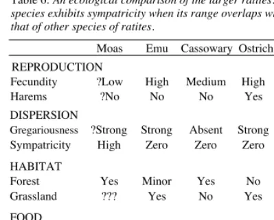
Table 6: An ecological comparison of the larger ratites. A species exhibits sympatricity when its range overlaps with that of other species of ratites.
Moas Emu Cassowary Ostrich Rhea REPRODUCTION
Fecundity ?Low High Medium High High
Harems ?No No No Yes Yes
DISPERSION
Gregariousness ?Strong Strong Absent Strong Strong Sympatricity High Zero Zero Zero Zero HABITAT
Forest Yes Minor Yes No No Grassland ??? Yes No Yes Yes FOOD
Fruits ?Yes Yes Yes Yes Yes Grass/forbs ?Yes Yes Minor Yes Yes Browse Yes Yes Minor Yes Yes Meat ??? Yes Minor Yes Yes
with an outline of those of the moas. The information on the ratites was gleaned from a variety of sources but, since my list had been checked and modified by John Calaby and Richard Schodde, I am confident that it is about right.
Table 6 shows that none of the extant large ratites provides a model of moa ecology. The moas were the only group of ratites that radiated to produce many forms whose ranges overlapped. The Emus did not. Nor did the cassowaries, the rheas, the ostriches, the Dromornithids or the elephant birds. Further, the moas were the only ratites that did not share their habitat with several unrelated herbivores. Cassowaries are the only forest-dwelling birds among the larger extant ratites, but in almost all other respects the life style of cassowaries contrasts with that of the moas. Cassowaries are forest-floor scavengers, and that is a good way of earning a living only in the tropics where fruit falls throughout the year; moas were browsers. Cassowaries are solitary; moas were probably gregarious, as are emus, ostriches and rheas.
The extant large ratites provide no ecological analogue of the moas, particularly with respect to their relationship with the plants. If we seek one nonetheless, we must search for it among other taxa. The best I can come up with, by no means an exact match, is the suite of mammals comprising kudu Tragelaphus strepsesceros, bushbuck Tragelaphus scriptus and duiker Sylvicapra grimmia. Another possibility is the suite of browser-grazers comprising roe deer Capreolus capreolus, fallow deer Dama dama and red deer Cervus elaphus.
AD 1000 to AD 1800 - Polynesian
Colonisation and the Extinction of Moas
The colonisation of New Zealand by the Polynesians was an ecological revolution. They brought with them six species of plants and two species of mammals. Their homeland was in the east of Polynesia, but present evidence is insufficient to identify it more tightly than within that vast expanse of ocean containing the Marquesas Group, the Society Islands and the South Cooks (Green, 1975). Wherever it was precisely, the open ocean crossing clearly exceeded 3000 km. Lewis (1977) suspects that their direction of search was set for them by the migratory flight-path of the long-tailed cuckoo Eudynamis taitensis, a suspicion I consider entirely plausible on the evidence of navigational methods used by the Polynesians of the central Pacific at the time of European contact.
During the phase of population increase and the consequent colonisation of unoccupied territory the New Zealand mainland lost its sea lions and sea elephants, and about 25 species of birds including the II species of moa. The mechanism of extinction is not relevant to the purposes of this symposium; here I simply note its occurrence and its tight association with the arrival of the Polynesians. The extinction of the moas was a brief passage in historical time, a wink in ecological time, and instantaneous in geological time. After about AD 1400 the major New Zealand grazing systems ceased to exist, their place taken by an unbrowsed vegetation that had to adjust to that new regime. The Polynesians did not just eliminate the moas, they eliminated an ecological and evolutionary process developed over more than 50 million years. We know roughly what the vegetation was converted to because we have Cockayne's (1921) descriptions from the days before the deer, but we do not know much about what it was converted from. First principles of range management inform us that, during the interregnum between the moas departing and the deer arriving, the 'decreaser species' would have out-competed the 'increaser species'. They would have proliferated at the expense of the latter, and would have banished 'invader species' from many plant communities. But we have scant information on which plant species fitted into each of those categories under the regime of defoliation enforced by the moas.
AD 1800 onward - New Plant-herbivore
Systems
was again browsed and grazed, this time by a suite of mammalian herbivores from the northern hemisphere, reinforced by selected marsupials from across the Tasman. Each of these species had a feeding niche that would have differed in detail from those of each moa species, and the possum (Trichosurus vulpecula) took up a niche almost without counterpart within the original biota. The effect of these animals on the aberrant plant communities that formed in the absence of both moas and deer has been documented in some detail. It need not be reviewed here.
Discussion
So far I have dealt loosely with the theme of plant-herbivore systems. If I have tried to get any message across it is that a plant-herbivore system is not simply a vegetation suffering the misfortune of animals eating it. Rather it is an interactive system with massive feed-back loops between the dynamics of the plants and the dynamics of the animals. Any disruption of those loops changes the system profoundly.
A vegetation plot deprived of grazing and browsing shows the effect of those processes upon the vegetation. (We might note that the complementary experiment - herbivores deprived of vegetation - is less frequently mounted.) If the exclosure experiment is designed correctly there will be an unprotected control plot with which the protected plot is compared. Suppose those two plots were in Kenya. The vegetation of the control plot outside the fence would be seen as normal in structure and composition, that within the fence as an aberration reflecting an abnormal environment. In New Zealand the more likely characterisation would be 'normal' for inside and 'aberrant' for outside, and that would be only half wrong. Outside is certainly aberrant with respect to the species composition as it was in AD 1000, but inside is normal with respect to nothing. We older New Zealand biologists made the mistake up to about the middle sixties of equating the inside of a protected plot with biological normality. The common view then was that the vegetation was vulnerable to grazing and browsing, that moas had passed away millenia ago, that they chiefly lived in grassland, that their effect on the forest was minimal, and that they were
uncommon. The moas were seen as ancient, sparse and ineffectual, having no relevance to the problems of today. The re-thinking began with Fleming's (1962) demonstration that moas became extinct
comparatively recently.
The introduction of any new herbivore changes an ecosystem. Deer are no exception. They changed the
then composition of the New Zealand vegetation. Taking a herbivore out of an ecosystem also changes plant associations. The erection of an exclosure almost anywhere in the world causes marked and usually rapid changes in species composition. On this basis we can deduce with some confidence that the extinction of the moas about AD 1400 changed the structure and species composition of the vegetation. If their removal did not have such an effect then those plant-herbivore systems differed radically from any others known to science. Moas would not have had the same effect as deer. I do not know of two herbivore species' anywhere whose effect on vegetation is equivalent. Most areas of New Zealand apparently hosted several species of moa. Those forms differed considerably in size, almost certainly had different feeding niches, and would themselves have affected the vegetation in different ways.
I suspect that my outline thus far will not generate much controversy because most of it is simply a review of published information. The little that could be described as new contains few surprises, and my interpretations hold close to current orthodoxy. The next step however is to decide what to do with that information, and I would suggest that such decisions are not logical extrapolations from data but instead are judgements of value. This is the murky realm of value systems and beliefs, the domain of the social anthropologist rather than of the ecologist.
There are three forms of belief that differ in kind, and I illustrate them with examples:
(a) Moas died out before Polynesians arrived. (b) Polynesians hunted the moas to extinction. (c) Deer improve/damage the New Zealand vegetation.
The first proposition is a hypothesis in that it is potentially falsifiable. We may argue its pros and cons vehemently but only until the data are in. Then there is no argument.
The second is not vulnerable to a knock-down test. It is not a hypothesis but a paradigm. Whether we accept it or reject it depends on a judgement of the weight and weighting of circumstantial evidence.
always framed in abstract terms.
A first cousin of ideology is the idealised goal that cannot be attained in practice, but which is
nonetheless actively pursued on the assumption that the closer it is approached the more successful is the exercise. But the solution of a great many ecological problems does not lie along one dimension. Often there are at least two solutions, of roughly equivalent efficacy, to a problem of applied ecology. A common characteristic of such multi-dimensional and non-linear systems is that whereas either of two management strategies will work, a compromise between them, or an approach to one that never gets there, will be unsuccessful. The first rule of applied ecology goes: if at first you don't succeed you have misunderstood the dynamics of the system.
As an example I contrast feasible management options for thar Hemitragus jemlahieus and red deer Cervus elaphus. Those for thar are the broader: we can choose to remove that species from the mountains of New Zealand or we can choose to retain it. If the latter be chosen, a further set of options within that choice becomes available. If the former, neither technical nor financial constraints stand in the way. My rough estimate of the cost of removing thar is twenty-four million dollars expended over 2 _ years. That may appear a large sum but it is no more than the cost of a modest block of offices or of 8 km of motorway. Governments make financial decisions of that size once a week. Treasury's predictable
compromise of eighteen million dollars over five years is not a practical option because, if I have costed the exploitation dynamics about right, it would not remove all the thar. Money down the drain.
In contrast, complete removal is not an option for red deer. It is not feasible because of the realities of distribution, terrain and habitat. Hence there is no place in policy for that ultimate aim because the management activities flowing from its adoption would block those options that are feasible. Equally unsatisfactory is the non-policy that fails to identify feasible options and which is no more than a
continuing administrative reaction to fluctuating social and economic pressures.
Management options must be stated in concrete form and anchored in ecological and geographic fact if they are to be anything more than wishful fancy. The appropriate density of deer in a given area is neither that 'commensurate with wise land use', nor that 'consistent with the continuing health of the forest', nor some similar metaphysical construct. It is a specifiable level, indexed or measured, that meets
the precisely defined management aims for the ecological system of that area.
The burden of reducing management options to those technically feasible is lightened by the injection into that process of a little technical expertise. That has not always been sought or offered previously. Only when feasible options are identified, and the social, economic, aesthetic and environmental impact of each assessed, is anyone in a position to make an informed choice.
We must not change reality to fit ideology.
References
Anderson, A. 1983. Faunal depletion and
subsistence change in the early history of southern New Zealand. Archaeology in Oceania 18: 1-10. Anderson, A. 1984. The extinction of moa
in southern New Zealand. In: Martin, P .S.; Klein, R.G. (Editors). Quaternary extinctions: a prehistoric revolution. pp 728-740. University of Arizona Press, Tucson.
Bell, C.J.E.; Bell, I. 1971. Subfossil moa and other remains near Mt. Owen, Nelson. New Zealand Journal of Science 14: 749-758. Bell, R.H.V. 1982. The effect of soil nutrient
availability on community structure in African ecosystems. In: Huntley, B.J.; Walker, B.H. (Editors). Ecology of tropical savannas. Pp 193-216. Springer-Verlag, Berlin. Botkin, D.B.; Mellilo, J.M.; Wu, L. S.-Y.
1982. How ecosystem processes are linked to large mammal population dynamics. In: Fowler, C.W.; Smith, T.D. (Editors). Dynamics of large mammal populations. pp 373-387. John Wiley and Sons, New York.
Burrows, C.J.; McCulloch, B.; Trotter, M. M. 1981. The diet of moas. Records of the Canterbury Museum 9: 309-336. Caughley, G.; Krebs, C.J. 1983. Are big
mammals simply little mammals writ large. Oecologia 59: 7-17.
Cockayne, L. 1921. The vegetation of New Zealand. Engelmann, Leipzig.
Coe, M.J.; Cumming, D.M.; Phillipson, J. 1976. Biomass and production of large African herbivores in relation to rainfall and primary production. Oecologia 22: 341-354. Cracraft, J. 1976. The species of moas
(Aves:Dinornithidae). Smithsonian Contributions to Paleobiology 27: 189-205.
Falla, R.A. 1962. The moa, zoological and archaeological. New Zealand Archaeological Association Newsletter 5: 189-191.
Fleming, C.A. 1962. The extinction of moas and other animals during the Holocene period. Notornis 10: 113-117.
Fleming, C.A. 1969. Rats and moa extinction. Notornis 16: 210-211. Golson, J. 1957. New Zealand archaeology
1957. Journal of the Polynesian Society 66: 271-290.
Green, R.C. 1975. Adaptation and change in Maori culture. In: Kuschel, G. (Editor). Biogeography and ecology in New Zealand. pp 591-641. Monographiae Biologica No. 27, Junk, The Hague.
Hartree, W.H. 1960. A brief note on the stratigraphy of bird and human material in Hawkes Bay. New Zealand Archaeological Association Newsletter 3: 28.
Horn, P.L. 1983. Subfossil avian deposits
from Poukawa, Hawkes Bay, and the first record of Oxyura australis (Blue-billed Duck) from New Zealand. Journal of the Royal Society of New Zealand 13: 67-78.
Lewis, D. 1977. From Maui to Cook. DOubleday, Sydney.
McGlone, M.S. 1978. Forest destruction by early Polynesians, Lake Poukawa, Hawkes Bay, New Zealand. Journal of the Royal Society of New Zealand 8: 275-281.
Millener, P.R: 1982. And then there were twelve: the taxonomic status of Anomalopteryx oweni (Aves: Dinornithidae). Notornis 29: 165-170.
Mills, J.A.; Lavers, R.B.; Lee, W.G. 1984. The takahe - a relict of the Pleistocene grassland avifauna of New Zealand. New Zealand Journal of Ecology 7: 57-70.
Trotter, M.M. 1979. Tai Rua: A moa-hunter site in north Otago. In: Anderson, A. (Editor). Birds of a feather. pp 203-230. British Archaeological Reports International Series No. 62.
Trotter, M.M.; McCulloch, B. 1984. Moas, men, and middens. In: Martin, P.S.; Klein, R.G. (Editors). Quaternary extinctions: a prehistoric revolution. pp 708-727. University of Arizona Press, Tucson. Oliver, W.R.B. 1949. The moas of New Zealand and
Australia. Dominion Museum Bulletin No. 15: 1-206.
Pielou, E.C. 1969. An introduction to mathematical ecology. Wiley-Interscience, New York. moa genus Megalapteryx. Notornis 35: 99-108. Worthy, T.H. 1988b. An illustrated key to the
main leg bones of moas. National Museum of New Zealand Miscellaneous Series. No. 17. Yaldwyn, J.C. 1979. The types of W.R.B. Oliver's
moas and notes on Oliver's methods of measuring moa bones. In: Anderson, A. (Editor). Birds of a feather. pp 203-230. British Archaeological Reports International Series No. 62. Yule, G.U. 1912. On the methods of measuring