DESIGN
by
Mahamudul Hasan
A thesis
submitted in partial fulfillment of the requirements for the degree of Master of Science in Civil Engineering
Boise State University
DEFENSE COMMITTEE AND FINAL READING APPROVALS
of the thesis submitted by
Mahamudul Hasan
Thesis Title: Exploring the use of data from newer technologies in road design Date of Final Oral Examination: 22 July 2019
The following individuals read and discussed the thesis submitted by student Mahamudul Hasan, and they evaluated his presentation and response to questions during the final oral examination. They found that the student passed the final oral examination.
Mandar Khanal, Ph.D., P.E. Chair, Supervisory Committee Bhaskar Chittoori, Ph.D., P.E. Member, Supervisory Committee Mojtaba Sadegh, Ph.D. Member, Supervisory Committee
iv
v
First, I would like to say a very big thank you to my supervisor Dr. Mandar Khanal, who always encourages me to look for something innovative. His dedication and keen interest; above all his overwhelming attitude to help me had been solely and mainly responsible for completing my thesis. Without his guidance and persistent help, completing this milestone would not have been possible. He isn't just a mentor to me yet in addition he resembles a father to me.
I am also grateful to Dr. Bhaskar Chittoori and Dr. Mojtaba Sadegh for their kind support, good advice and kind appreciation. I would like to give my exceptional gratitude to Mr. Nikolaus W. Sterbentz from Idaho Transportation Department (ITD) for his caring help and direction for Lidar and UAV data analysis. Special thanks to Mr. Ryen Johnson from ITD for his thoughtful help to analyze the Lidar data.
I am grateful to Aero-Graphics, R.E.Y. Engineers and Dioptra Geomatics for their successful effort in collecting the Aerial Lidar, Mobile Lidar and Validation Survey data respectively. Without the use of these data, this research would not be completed.
vi
lot for me. Special thanks to my father who kept his confidence on me during my hardest time.
vii
The use of Light Detection and Ranging (Lidar) is widespread currently all over the world including the United States. Though on-the-ground surveying and photogrammetric surveying are the more common methods to acquire terrain information, Lidar data is being increasingly used for this purpose due to its various advantages. Various research indicates that the accuracy of Lidar data has increased enough to make its use suitable for diverse applications. One potential application that is explored in this research is the use of terrain models generated from Lidar data in road design. To make such use possible we need to be assured that the accuracy of terrain models developed from Lidar data is comparable to models obtained from traditional land surveying techniques. Such assertions were tested in this research.
viii
ix
DEDICATION ... iv
ACKNOWLEDGMENTS ... v
ABSTRACT ...vii
TABLE OF CONTENTS ... ix
LIST OF TABLES ...xii
LIST OF FIGURES ... xiii
CHAPTER ONE: INTRODUCTION AND BACKGROUND ... 1
Statement of Problem ... 1
Background ... 3
Research Objectives and Tasks ... 6
Organization of Thesis ... 7
References ... 8
CHAPTER TWO: MANUSCRIPT ONE – STATISTICAL ACCURACY COMPARISON OF AERIAL LIDAR, MOBILE-TERRESTRIAL LIDAR, AND UAV PHOTOGRAMMETRIC CAPTURE DATA ELEVATIONS OVER DIFFERENT TERRAIN TYPES... 9
Abstract ... 9
Introduction ... 10
Methods ... 12
x
Data Collection ... 14
Mobile-Terrestrial Lidar ... 14
UAV Photogrammetric Data Capture ... 15
Verification Survey ... 17
Analysis ... 17
Results... 21
Statistical Analysis ... 28
Cost Comparison ... 30
Conclusions ... 32
Acknowledgments... 33
References ... 33
CHAPTER THREE: MANUSCRIPT TWO – ROAD DESIGN USING ALTERNATIVE DATA SOURCES ... 36
Abstract ... 36
Introduction ... 37
Study Area ... 40
Study Objectives ... 41
Methodology ... 42
Data Collection ... 42
Airborne Lidar ... 42
Terrestrial Mobile Lidar ... 43
UAV... 43
xi
OpedRoad Designer... 44
Results and Discussion ... 47
Statistical Analysis ... 52
Two Tailed Z-Tests ... 52
Aerial Lidar and Survey Data ... 52
Mobile Lidar and Survey data ... 52
UAV-Based Lidar and Survey data ... 53
Cost Comparison... 53
Conclusions and Recommendations ... 54
Limitations of the Study ... 55
Acknowledgments... 55
References ... 55
CHAPTER FOUR: SUMMARY, CONCLUSIONS, AND RECOMMENDATIONS .... 57
Summary and Conclusions ... 57
xii
Table 2.1 Statistics Related to Difference in Elevations for Different Data Sources 21 Table 2.2 Statistics Related to Difference in Elevations for Three Sections ... 22 Table 2.3 Statistics Related to Difference in Elevations for Road-Surface and
Non-Road-Surface Survey Points ... 24 Table 2.4 Statistics Related to Difference in Elevations for Three Slope Areas ... 25 Table 2.5 Cost comparison of each data source type ... 30 Table 3.1 Statistics Related to Overall Difference in Elevations for Different Data
Sources ... 48 Table 3.2 Statistics Related to Difference in Elevations for Three Sections ... 49 Table 3.3 Statistics Related to Difference in Elevations for Road-Surface and
xiii
Figure 2.1 Google Earth image of the study area ... 13 Figure 2.2 Classified aerial lidar data ... 19 Figure 2.3 Survey points imported in ArcMap ... 20
Figure 2.4 RMSE comparison by data type, location on/off road surface, and terrain slope ... 28 Figure 3.1: GOOGLE EARTH IMAGE of the STUDY AREA ... 41 Figure 3.2 SURVEY POINTS IMPORTED in OPENROADS DESIGNER for ONE
SECTION of OUR STUDY AREA ... 47 Figure 3.3 RMSE FOR DIFFERENT TYPES of DATASETS BASED on
CHAPTER ONE: INTRODUCTION AND BACKGROUND Statement of Problem
Since the introduction of motor vehicles, roads have become one of the basic pillars of a modern society. Today many of the citizens in the United States of America (USA) are the owner of their own vehicles. People use their vehicles over road networks for various personal reasons; the road network is also used to move goods to consumers. It is said that for the development of a country, developing the road network is one of the basic steps. This is especially true for less developed countries of the world. Also, during the time of building the roads we need to think about preserving the operability of the road network while considering the safety of the road users. For these reasons, road design is a critical endeavor and we have to be very cautious when we design a road network.
information. In unfavorable climate conditions, it is even harder to get the required information using these methods.
Because of the various complexities associated with traditional methods, there has always been a demand for alternative methods for terrain data collection. One of the most promising alternatives is the use of Light Detection and Ranging (LIDAR) for collecting terrain data. LIDAR is one of the most innovative remote sensing terrain mapping technologies. In most of the cases, Digital Surface Model (DSM) represents the earth's surface. DSM is a surface model which contains practically all sort of objects on the surface. For road design we need the information about elevation of the study area. For this, a Digital Terrain Model (DTM) is ideal. A DTM represents the bare surface ground without any kind of objects above the ground like plants, cables or buildings (1). This accurate DTM is a very important source of data for Geographic Information Systems (GIS). It can be used for many studies such as assessing terrain parameters, analyzing the earth’s surface, performing spatial analysis, and also for building other spatial models.
This type of data is used for engineering and environmental analysis purposes. At present, there are quite a few data sources for generating the DTM. The most widely used and most common method is the classical field survey and it is usually done with the use of total stations or Global Navigation Satellite System (GNSS) receivers. The accuracy of the data resulting from this method is high. The method is expensive (2) and time consuming (3). For creating the DTM, LIDAR can be an effective alternative.
classical techniques. UAV is a relatively newer type of remote-sensing platform which has significant advantages over conventional piloted aircrafts and satellites. The most important advantages of this method are low cost, operational flexibility, and better spatial and temporal resolutions. Primarily drones are used to collect the UAV data. As they can be easily operated, less time will be needed for collecting the data. For these reasons, this method is expected to be the lowest-cost alternative relative to the other alternatives. Our literature review revealed, however, that very few studies were found that compared these alternatives with traditional field surveying, which was quite surprising. Our goal is to find alternatives to the present surveying method, which will not only save time but is also less expensive. In this research, we have evaluated the effectiveness of the alternatives in terms of accuracy and cost.
Background
Three collection methods are presently utilized by many Departments of Transportation (DOT) for large scale elevation data collection:
1. Electronic Distance Measurement methods (Total Station), 2. Real Time Kinematic (RTK) methods
3. Photogrammetry.
Both Electronic Distance Measuring (EDM) and RTK strategies share comparable advantages and disadvantages, including:
Advantages:
• Electronic gathering in field permits quick download of information in
office
• Several units working autonomously take into consideration quick
information accumulation, particularly in unobstructed areas (e.g. fields) Disadvantages:
• Frequent equipment movements
• Permission required to access private property
• Personnel may work in risky territories (for example near roadways, heavy
traffic zones)
• Ineffective in zones where signs can be blocked (Forests, urban
communities, and so forth.)
Photogrammetry can address a portion of these disadvantages, yet it likewise has a few impediments. The symbolism for photogrammetric information should be taken in leaf-off conditions with no ice superficially. Leaf-off means that there is no foliage or a reduced amount of foliage on the tree. There is likewise a requirement for an appropriate sun edge with no cloud. That implies a compact time frame should be accessible to take the picture, which is not advantageous. Additionally, the procedure for getting heights from the pictures is moderate. Thus, there is a need to find an alternative that is quicker and less costly.
road design, disaster management, infrastructure inspection, environmental monitoring, traffic operations, and surveillance. As current surveying methods are lengthy and costly, various DOTs have been seriously looking for alternatives. In many cases, these alternative data need not have pinpoint accuracy in applications such as traffic operations or environmental monitoring. For utilizing these information sources, we should be cautious about the precision of the data dependent on the areas in which we intend to utilize this information. If the accuracy is not acceptable, then it can become problematic in many ways. For example, inaccurate LIDAR data can give inaccurate elevations for the study area. So, after designing the road when we start construction, we will have to change our design plans because of a wrong DTM for that area. In the worst case scenario it may require us to completely redesign the road or may need some substantial changes in the current design. Besides requiring more time to complete the project it will also increase the cost of the project. That is why we need to be certain about the accuracy of the alternatives before using them.
information exactness changes by land spread conditions (8). It is likewise asserted that LiDAR information exactness in flat zones are twice as precise as those in more steep zones with woodland inclusion (8).The research reported in this thesis tests that assertion by examining the applicability of Aerial Lidar, Mobile Lidar and Lidar data from UAVs as a function of ground slope.
Research Objectives and Tasks
The research hypothesis of this thesis is that Mobile Lidar data is more accurate than Aerial Lidar data. However, none of the Lidar data or UAV-based Lidar data can replace traditional survey data. In this study we try to find the answers to these questions:
• How can we compare the accuracy for different Digital terrain Models (DTM)?
• Up until what stage of road design are data from such newer technologies
acceptable?
• Will the alternatives be cost effective and save time?
To validate the hypothesis and to answer the above questions we consider several objectives for our research. They are:
1) Finding alternatives for traditional surveys 2) Comparing the accuracy of the alternatives 3) Statistical comparison of different surfaces 4) Evaluating the effectiveness of the alternatives
Our tasks to accomplish these research objectives and answer our questions are: i. Ground Survey, Aerial LIDAR, and Mobile Terrestrial LIDAR data were
ii. Digital Terrain Models (DTM) were generated from datasets in OpenRoads Designer Software. Also, ground survey points were imported with specific coordinates and elevations for the points were extracted using other data sources; the two sets of elevations were compared.
iii. A similar process was completed using the ArcMAP software. Then Digital Elevation Models (DEMs) were created from these processed files.
iv. Surveying points were imported in our study area and the elevations were again extracted for different files in ArcMAP.
v. The study area was divided into three categories.
vi. Overall accuracy for the study area as well as the accuracy for the sub-areas were estimated.
Organization of Thesis
References
1. Li, Z., Zhu, Q. and Gold, C. 2005. Digital terrain modeling:principles and methodology. CRC Press. Boca Raton
2. Grala, N. and Brach, M. 2009. Analysis of GNSS receiver inthe forest environment. Annals of Geomatics VII, 32(2):41-45
3. Yakar, M. 2009. Digital elevation model generation by ro-botic total station instrument. Experimental Techniques33(2): 52-59
4. Sithole, G.; Vosselman, G. Comparison of filtering algorithms. Int. Arch. Photogramm. Remote Sens. Spat. Inf. Sci. 2003, 34, 71–78.
5. Zhang, Y.; Men, L. Study of the airborne LIDAR data filtering methods. In Proceedings of the International Conference on Geoinformatics: Giscience in Change, Beijing, China, 18–20 June 2010.
6. Liu, X.Y. Airborne LiDAR for DEM generation: Some critical issues. Prog. Phys. Geogr. 2008, 32, 31–49.
7. Meng, X.; Currit, N.; Zhao, K. Ground Filtering Algorithms for Airborne LiDAR Data: A Review of Critical Issues. Remote Sens. 2010, 2, 833–860.
CHAPTER TWO: MANUSCRIPT ONE – STATISTICAL ACCURACY COMPARISON OF AERIAL LIDAR, MOBILE-TERRESTRIAL LIDAR, AND UAV
PHOTOGRAMMETRIC CAPTURE DATA ELEVATIONS OVER DIFFERENT TERRAIN TYPES
Abstract
Introduction
Designing new or existing transportation facilities requires accurate surface terrain information (1). Conventional survey methods for acquiring accurate terrain surfaces include Real Time Kinematic Global Positioning System (RTK-GPS), Electronic Distance Measurement (Total Station), and photogrammetry. Generally, RTK-GPS and Total Station procedures are time-consuming and costly due to the necessity of workers and equipment needing to physically move across the terrain of an area to achieve satisfactory coverage. Certain operational constraints such as dense vegetation cover must also be considered, and in the case of conventional surveys on existing road design projects, vehicular traffic is a further safety consideration. While large-area terrain information can be collected through these methods, the time and effort needed is significant.
Photogrammetry circumvents some of the limitations of RTK-GPS and Total Station survey but introduces other issues. Imagery used for photogrammetric data must typically be gathered in highly specific conditions, usually when foliage is in a bare, leaf-off state but before the ground is covered by snow and ice (1). Photogrammetry also requires a particular sun angle with no cloud cover present. Once photogrammetric imagery is collected, processing the data and determining elevation is often time-consuming.
mounting a lidar device on an aircraft or ground-based vehicle and moving while the device continuously collects point data. The result is a “point cloud” dataset of lidar point locations, from which elevation models can be created. Compared to the previously described conventional survey methods, lidar is generally considered to offer safer data collection, cost effectiveness, and a high level of detail (2).
Another remote sensing technique is the use of an unmanned aerial vehicle (UAV) to acquire photogrammetric capture data through the collection of a large volume of photographs. This method utilizes a digital structure from motion process with scale invariant feature transform tools. Essentially, this uses the oblique differences between photographs to generate a three-dimensional model of its target. A digital surface terrain model can be generated using this output, as well as a point cloud file or files resembling a lidar point cloud dataset. Although this method has some of the same issues as “traditional” photogrammetry, it is generally considered a less-expensive alternative to both conventional survey and lidar.
account a variety of factors including the multiple returns lidar typically produces (5). For example, classifying lidar data allows for differentiating between the ground, foliage, buildings, and water surface in the point cloud. Besides roadway design, lidar is routinely used in a variety of applications including forest inventory and assessment (6, 7), hydrologic channeling (8), and carbon sequestration (9).
Lidar used for roadway design is usually collected expressly for this purpose, and studies (3, 4, 10) have shown a root mean square error (RMSE) of 0.15–0.40m for vertical accuracy and horizontal RMSE of 0.5–1.0 m is achievable with lidar. The accuracy of lidar-derived digital elevation model (DEM) rasters has been researched over a variety of vegetation and terrain types (11). One study indicates that increasing terrain slope leads to lower lidar canopy height estimates because slope has effect on DEM accuracy (12). As part of this study, the effects of both slope and terrain type on lidar vertical accuracy will be examined.
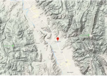
Methods Study Area
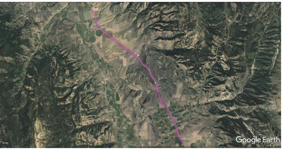
capture data covering the same general areas. All four datasets (aerial lidar, mobile-terrestrial lidar, UAV photogrammetric capture, and traditional survey cross-section points) were obtained from ITD. Figure 2.1 shows the study area.
Study Objectives
Several objectives were considered for this study:
1) Comparing the vertical accuracy of the three test case datasets to traditional survey elevation ground points,
2) Statistically determining whether the elevation differences between the test datasets are potentially acceptable for use in roadway design, and
3) Performing a cost analysis of the different data collection methods.
Data Collection Aerial Lidar
The aerial lidar data used in this study was collected between April 7 and October 12, 2016 by Aero-Graphics, as part of an ITD District 5 district-wide aerial lidar and imagery collection project. Aero-Graphics guaranteed the accuracy of these lidar data at “planning grade.” In order to achieve a greater degree of horizontal accuracy, survey control targets were strategically placed along collected routes districtwide (14). All data were collected using a custom districtwide coordinate projection, based on NAD 1983 Idaho State Plane East, intended to maintain regional measurement distances without needing to scale the data.
Collection was performed with an Optech ALTM Orion H300 sensor and an Optech CS-10000 aerial camera system, at an average 3,300 feet altitude. The lidar sensor and the camera were paired in a customized mount to improve accuracy and minimize error between datasets (14). Aero-Graphics reported a 30% overlap in the lidar data, yielding 9.6 points per square meter across the project. The pulse rate frequency used for the collection was 225 kHz with scan frequency of 68.7 Hz, and the scan angle was +/- 14.5° from the nadir position (full scan angle 29°). The Orion H300 was equipped with a GPS/IMU unit, recording the XYZ position and roll, pitch, and yaw attitude of the plane throughout the flight. This allowed for the correction of lidar returns that may have been thrown off by the plane’s motion during flight (14).
Mobile-Terrestrial Lidar
VMX-250 mobile scanning system, consisting of two RIEGL VQ-250 line scanners, two RIEGL CS6 5 MPx Cameras, 80°x65° FOV, an Applanix POS LV V5 Model 510 position and orientation system (IMU), a Trimble BD960 GNSS receiver, a Trimble Zephyr Model 2 GNSS Antenna, an Applanix Distance Measurement Indicator (DMI), and a RIEGL Control Unit (CU). For project control, Dioptra Geomatics set 110 control targets using RTK GPS, with the Utah Reference Network “TURN” solution to improve accuracy on most of these targets (15). These lidar data were collected as part of ITD project A019(382), from the Caribou county line to Nounan Road on US-30 in Bear Lake County. As a result, the data were collected using a custom coordinate system, based on NAD 1983 Idaho State Plane East, specific to the project. It should be noted that this coordinate system is different than the districtwide coordinate system used for the Aero-Graphics aerial lidar.
The collection vehicle with the VMX-250 scanning system was driven two times in each direction for data quality purposes, at an average speed of 35 miles per hour, varying between 30 and 40 miles per hour. Each scanner was set for a measurement rate of 300 kHz (600 kHz combined). For each pass at this speed, R.E.Y. reported a point density on the road surface of approximately 340 points/m2 at 20 feet away from the sensors, to over 2000 points/m2 along the trajectory line from the sensors as the point density were
collected (15). Unlike the aerial lidar data, the mobile-terrestrial lidar data did not have classifications assigned. Ground classification were determined for this study using the Classify LAS Ground tool in Esri ArcMap.
UAV Photogrammetric Data Capture
was flown at an average elevation of 151 feet above ground level using “terrain awareness” to follow features and create waypoints on the terrain based on a
NASA/USGS DEM from Mapbox. The UAV had a relative accuracy GPS/GLONASS system on board and was flown with an iOS mobile command and control application called Map Pilot. Two flights on each section were conducted on either side of the road with 75% front and side overlap and a solar elevation angle at nadir (solar noon) position for the particular date, derived from Spring/Fall NASA values. Approximately 330 aerial images were taken per road section at 3-second intervals. The image metadata Z-values (WGS84 EGM 96 Geoid) were manually adjusted in Microsoft Excel to correct the heights, and then processed in a key point matching process in Pix4D.
Nine aerial targets were set at each site to be used as ground control points, the coordinates of which were determined with a survey-grade RTK-GPS system using the same coordinate system and control point values as the on-the-ground survey data collection. The UAV-collected data was processed in Pix4D (including matching, extraction, densification, meshing, and scaling) utilizing Structure from Motion (SfM) and Scale Invariant Feature Transform (SIFT) tools to acquire a single image composed of the collected images. Using this composite, the program then produced 3D meshes and point clouds for each road section.
These produced data have a ground sampling distance of 1.5 cm/pixel. Pix4D calculated a root mean square error (in U.S. survey feet) of 0.56 for the data at the
Pix4D on the point cloud to filter out points besides the “road” and “ground” points to create a digital terrain model (DTM). A georeferenced DTM LAS point cloud file was then produced and used for the analysis process, exported to unmodified NAD 1983 State Plane Idaho East. No supplemental boundary work was performed on the outer edges of the imagery. It should be noted that the Pix4D unsupervised classification process was limited in its capability to classify the data; a second automated classification of ground returns only was performed using the Classify LAS Ground tool in Esri ArcMap.
Verification Survey
The conventional survey data used in this study to compare the elevational accuracies of the three remote data types was collected by Dioptra Geomatics between April and May 2017 using a Total Station. These cross-section points were collected for the purpose of verifying the accuracy of the mobile-terrestrial lidar and were collected using the same project-specific coordinate system. These verification surveys were used by R.E.Y. to examine the accuracy of the mobile-terrestrial lidar on pavement, at the edge of the pavement, and off-pavement ground using TopoDOT (15).
Analysis
to the conventional survey elevations for each point. The study road sections were subdivided into three categories to evaluate the effect of slope: level, moderate, and steep.
According to the AASHTO “Policy on Geometric Design of Highways and Streets” (commonly referred to as the “Green Book”), terrain with a slope between 0-2% is considered level, 2-5% is considered moderate, and slopes greater than 5% are considered steep. For the purposes of determining areas of level, moderate, and steep terrain for this analysis, degrees were used instead of percentage slope. Slope values less than 1⁰ were
categorized as level, between 1⁰ and 5⁰ were categorized as moderate, and more than 5⁰
were categorized as steep. The location of each point was categorized by this slope index. Root mean square error (RMSE) was calculated for all elevation differences between the conventional survey points and their corresponding locations on the test data DEM surfaces. These RMSE values were further divided by study road section, location on or off the road, and slope value.
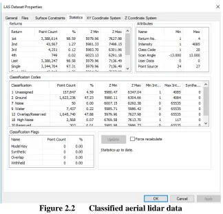
Figure 2.2 Classified aerial lidar data
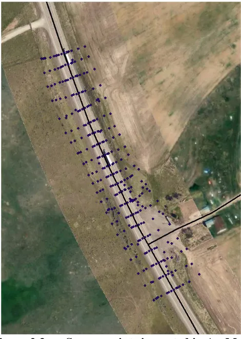
DEM surfaces were generated from the .las files, and these outputs were visually evaluated to ensure they covered the conventional survey points at each road section. Elevation data was then extracted from each DEM for each covered conventional survey point for aerial, mobile-terrestrial, and UAV data by using the Extract Values to Point (Spatial Analyst) tool. This process allowed for finding the elevations at the same horizontal points for the different data sources to statistically compare them. Figure 2.3 shows the survey points imported in ArcMap for a section of our study area.
RMSE was calculated for the differences between the surveyed elevation values and each DEM elevation value across all point locations. Further, RMSE was calculated for road-surface and non-road-road-surface points, and for each study road section independently.
Figure 2.3 Survey points imported in ArcMap
area. Slope values were then extracted for aerial, mobile-terrestrial, and UAV data at each survey point.
Results
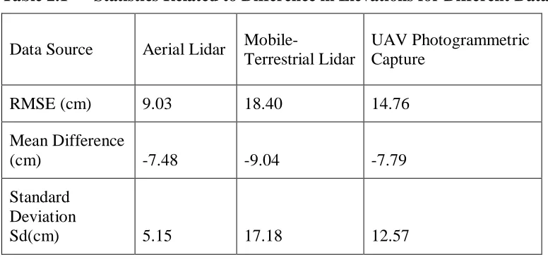
Table 2.1 shows the difference in elevations obtained from the conventional survey and each remote method DEM for all survey point locations using ArcMap. The conventional survey elevations were considered to be the “true” elevations.
Table 2.1 Statistics Related to Difference in Elevations for Different Data Sources
Data Source Aerial Lidar
Mobile-Terrestrial Lidar
UAV Photogrammetric Capture
RMSE (cm) 9.03 18.40 14.76
Mean Difference
(cm) -7.48 -9.04 -7.79
Standard Deviation
Sd(cm) 5.15 17.18 12.57
The difference in elevation represented in Table 2.1 is the conventional survey elevation minus the elevation obtained from one of the three remote sources of data. All elevation differences used in this table were taken into account, regardless of location or slope. The mean difference was found to be negative for all three remote data sources, indicating that on average the remote data sources overestimated the ground elevation. The table shows that the aerial lidar elevations are closer to the surveyed elevations than those from the other two sources. The RMSE for mobile-terrestrial lidar was the highest in this analysis, with similar results for mean difference and standard deviation.
Section 1. This was also true for mean difference except for the aerial lidar elevation differences. The accuracy was higher in Sections 2 and 3 for all remote data sources.
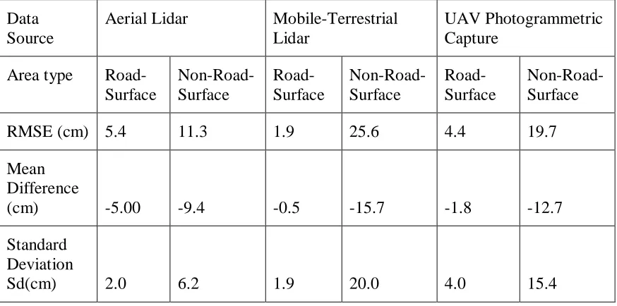
Table 2.3 presents the elevation differences for road- and non-road-surfaces. The RMSE for the road-surface points is much lower than that for the non-road-surface points. The RMSE for road-surface is quite acceptable within the standard accuracy limit stipulated by the Idaho Lidar Consortium (ILC). According to ILC, any RMSE less than 5 cm is within their accuracy standard. For points on the road-surface, mobile-terrestrial lidar gave the most accurate result among the three sources of data, while the aerial lidar had the highest RMSE (5.4 cm). The mean differences and standard deviations were also low for all remote data sources. It can be concluded that on road-surface areas, all these data types are capable of achieving acceptable results.
Table 2.3 Statistics Related to Difference in Elevations for Road-Surface and Non-Road-Surface Survey Points
Data Source
Aerial Lidar Mobile-Terrestrial Lidar
UAV Photogrammetric Capture
Area type Road-Surface
Non-Road-Surface
Road-Surface
Non-Road-Surface
Road-Surface
Non-Road-Surface
RMSE (cm) 5.4 11.3 1.9 25.6 4.4 19.7
Mean Difference
(cm) -5.00 -9.4 -0.5 -15.7 -1.8 -12.7
Standard Deviation
Sd(cm) 2.0 6.2 1.9 20.0 4.0 15.4
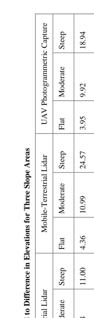
lower compared to those for the other two remote datasets. This, along with its RMSE of 7.48 cm for moderate areas, explains why the overall RMSE, all points considered, was lowest for the aerial lidar.
The RMSE for the mobile-terrestrial lidar was higher than aerial lidar for all types of terrain areas. A total of 920 conventional survey points was available for comparison of the mobile-terrestrial lidar. Of these 920 points, only 39 points were on ground considered level. The highest number of points were considered moderate, a total of 458. The remaining 423 points were considered steep. The mobile-terrestrial RMSE was 4.36 cm for level terrain, which was low compared to that for aerial lidar. The highest RMSE for mobile-terrestrial lidar was obtained in steep areas with an RMSE value of 24.57 cm, while in moderate areas the RMSE was 10.99 cm. The overall RMSE was high, due to the higher RMSE in the steep areas. Similar patterns are apparent in the mobile-terrestrial mean difference and standard deviation for each terrain type. All values were high for steep regions and low for level regions, following a pattern similar to the aerial lidar.
than the mobile-terrestrial lidar. The mean difference and standard deviation for the UAV data appear to generally follow the same patterns as for the aerial lidar and mobile-terrestrial lidar.
Figure 2.4 RMSE comparison by data type, location on/off road surface, and terrain slope
Statistical Analysis
Two tailed z-tests were performed for these for pairs of elevations. The null hypothesis (H0) was that the difference in the two elevations are within the ILC vertical
accuracy standard of 5 cm or 0.164 ft, and the alternative hypothesis (Ha) was that they are
not equal. One of the two elevations is the elevation for one of the alternative data sources, the other is the ground-survey elevation, which is considered to be the “true” elevation.
Define,
µd= Mean elevation difference between the datasets;
H0: µd = 0.164
Ha: µd≠ 0.164
0 5 10 15 20 25 30
RM
SE
(c
m
)
Zone Type
Aerial Lidar and Survey data H0: µd = 0.164
Ha: µd≠ 0.164
We found z= -73.6
For α=0.05, our obtained P value<0.00001
So, the null hypothesis, H0, can be rejected at the 5% level of significance. The
difference in elevations between the two sets of elevations are statistically not within the ILC standard.
Mobile Lidar and Survey data H0: µd = 0.164
Ha: µd≠ 0.164
We found z= -24.8075
For α=0.05, our obtained P value<0.00001
So, the null hypothesis, H0, can be rejected at the 5% level of significance. The two
sets of elevations are statistically not within the ILC vertical accuracy standard. UAV-Based Lidar and Survey data
H0: µd = 0.164
Ha: µd≠ 0.164
We found z= -30.9
For α=0.05, our obtained P value<0.00001
So, the null hypothesis, H0, can be rejected at the 5% level of significance. Again,
From this analysis it can be concluded that the elevations from the aerial lidar, mobile-terrestrial lidar and UAV photogrammetric data are statistically not close enough to the survey elevations using the ILC vertical accuracy standard.
Cost Comparison
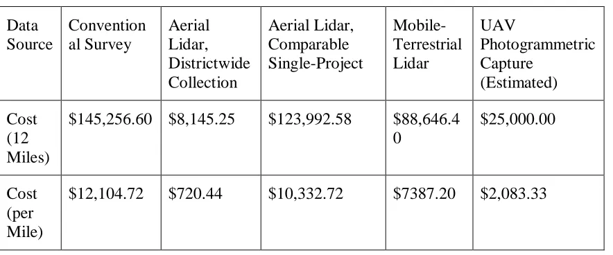
For the cost comparsion, the twelve miles of US-30 between mileposts 413 and 425 where the mobile-terrestrial lidar was collected in Bear Lake County are considered. Table 2.5 lists the costs of collecting and processing each data type for a roadway project of this magnitude:
Table 2.5 Cost comparison of each data source type Data Source Convention al Survey Aerial Lidar, Districtwide Collection Aerial Lidar, Comparable Single-Project Mobile-Terrestrial Lidar UAV Photogrammetric Capture (Estimated) Cost (12 Miles)
$145,256.60 $8,145.25 $123,992.58 $88,646.4 0
$25,000.00
Cost (per Mile)
$12,104.72 $720.44 $10,332.72 $7387.20 $2,083.33
5,280 feet x 12 miles = 63,360 feet/3,000 feet = 21.12 cross-sections x $6,877.68 = $145,256.60
The planning-grade aerial lidar used in this study is part of a districtwide collection effort, including 716 linear miles of roadway. Economies of scale are important to note in determining the cost of such an extensive project. The total cost of the project, including ground survey control by AeroGraphics’ survey crew, as well as the collection of aerial imagery by Aero-Graphics, Inc., orthorectified imagery, DEM raster surfaces, and other data processing, was $486,000, from which the 12-mile and single-mile figures are derived. However, if a consultant collected aerial lidar on a more limited basis at design-grade (as the mobile-terrestrial lidar was), rather than districtwide at planning-design-grade, the cost would likely be significantly more. This may in large part be due to the necessity of mobilizing the collection aircraft. To approximate this cost, a comparable aerial lidar collection effort such as that for ITD project keys 14002 and 13106, flown in 2014, could be used for comparison. The invoiced amount of the combined lidar collection for these projects was $123,992.58.
It should be noted that the comparison here is not perfectly analogous to the US-30 project area, as it is for a different part of the highway system, multiple stretches of highway, and includes numerous side roads, which may make for a more complex flight pattern. However, the total highway distance with these two roads is similar to the US-30 study area and should make for a reasonable comparison with the US-30 study area data costs.
Geomatics, was $88,646.40. This collection spanned 12 highway miles between MP 413-425 on US-30. Finally, because the UAV photogrammetric data was collected and processed in-house by ITD, the cost in the table is an approximate estimate of the cost by a consultant.
Conclusions
Although all three remote data sources deviated from the conventionally-surveyed elevations, the mobile-terrestrial lidar was particularly close on the road surface. The aerial lidar, while guaranteed at planning-grade, also proved promisingly close on the road surface, as did the UAV photogrammetric data. For this reason, the UAV photogrammetric data capture method may be a cost-effective alternative to the other two remote data types. All three remote data types may be suitable for certain design purposes, particularly preliminary design and those dealing primarily with an existing road surface.
The accuracy of each data type degraded at higher steepness and off-pavement. Spaete et al. noted that vegetation and slope areas have a statistically significant impact on the accuracy of lidar-derived DEMs (13). This study indicates that the aerial lidar provided the most accurate terrain information in these areas. Considering the vantage point of the aerial lidar with its capability of multiple returns, this makes sense. The mobile-terrestrial lidar is understandably limited by its ground vantage point, especially in areas with steep slopes.
accuracy. Another possible consideration is the processing method each remote .las dataset received. The aerial lidar received some manual processing, while the mobile-terrestrial and UAV data both relied on an automated ground-classifying process in ArcMap. Manual processing of the mobile-terrestrial lidar and UAV photogrammetric data may improve the accuracy of these data types in off-road and steeper areas.
Acknowledgments
The authors would like to thank the Idaho Transportation Department for providing the data for use in this study.
References
1. Veneziano, D., Souleyrette, R., and S. Hallmark. Evaluation of Lidar for Highway Planning, Location, and Design. Proc., 4th Int. Conf. Pecora 15/Land Satellite Information IV ISPRS, (CD ROM), American Society for Photogrammetry & Remote Sensing, Denver, 2002. doi: https://www.researchgate.net/publication/238620013
2. Chang, J. C., Findley, D. J., Cunningham, C.M., and M. K. Tsai. Considerations for Effective Lidar Deployment by Transportation Agencies. Transportation
Research Record: Journal of the Transportation Research Board, 2014. 2440: 1-8.
3. Pourali, S. H., Arrowsmith, C., Chrisman, N. R. and A. Matkan. Vertical Accuracy Assessment of Lidar Ground Points Using Minimum Distance Approach. CEUR
Workshop Proceedings, 2014. 1142: 86-96.
4. Hodgson, M. E. and P. Bresnahan. Accuracy of Airborne Lidar-Derived Elevation: Empirical Assessment and Error Budget. Photogrammetric Engineering and
Remote Sensing, 2004. 70(3): 331-340.
5. Cui, Z. A Generalized Adaptive Mathematical Morphological Filter for LIDAR Data. FIU Electronic Theses and Dissertations, 2013. 995.
6. Goodwin, N.R., Coops, N.C., and D. S. Culvenor. Assessment of Forest Structure with Airborne LiDAR and the Effects of Platform Altitude. Remote Sensing of
7. Smith, A. M. S., Falkowski, M. J., Hudak, A. T., Evans, J. S., Robinson, A.P., and C. M. Steele. A Cross-Comparison of Field, Spectral, and Lidar Estimates of Forest Canopy Cover. Canadian Journal of Remote Sensing, 2009. 35(5): 447–459. doi:10.5589/m09-038
8. Bowen, Z. H., and R.G. Waltermire. Evaluation of Light Detection and Ranging (LiDAR) for Measuring River Corridor Topography. Journal of American Water Resources Association, 2002. 38(1): 33–41. doi: 10. 1111/j.1752-1688.2002.tb01532.x.
9. Asner, G.P. Tropical Forest Carbon Assessment: Integrating Satellite and Airborne Mapping Approaches. Environmental Research Letters, 2009. 4(3): 034009. doi: 10.1088/1748-9326/4/3/034009
10. Shrestha, R. L., Carter, W. E., Lee, M., Finer, P., and M. Sartori. Airborne Laser Swath Mapping: Accuracy Assessment for Surveying and Mapping Applications. J. Am. Congr. on Surv. and Mapping, 1999. 59(2): 83–94.
11. Tinkham, W. T., Huang, H., Smith, A. M. S., Shrestha, R., Falkowski, M. J., Hudak, A. T., Link, T. E., Glenn, N.F., and D. G. Marks. A Comparison of Two Open Source Lidar Surface Classification Algorithms. Remote Sensing, 2011. 3(3): 638– 649. doi: 10.3390/rs3030638.
12. Gatziolis, D., Fried, J.S., and V. S. Monleon. Challenges to Estimating Tree Height via Lidar in Closed-Canopy Forests: A Parable from Western Oregon. Forest
Science, 2010. 56(2): 139–155.
13. Spaete, L. P., Glenn, N. F., Derryberry. D. R., Sankey, T. T., Mitchell, J. J., and S. P. Hardegree. Vegetation and Slope Effects on Accuracy of a Lidar-Derived DEM in the Sagebrush Steppe. Remote Sensing Letters, 2011. 2(4): 317-326.
14. Technical Project Report: D5 Aerial Photography and Lidar, Project Nos. A014(008), A014(009) and Key Nos. 14008, 14009. Submitted to ITD by Aero-Graphics. April 2016 - August 2017. 33 pages.
CHAPTER THREE: MANUSCRIPT TWO – ROAD DESIGN USING ALTERNATIVE DATA SOURCES
Abstract
Introduction
We use different types of transportation modes in our daily life. Transport modes are the means by which passengers and freight achieve mobility. Roads, rails, waterways,
and airways are the most common modes of transportation. Among all modes, roads play
a vital role in the development of a country. Roads are vital for economic development of
a country and provide many social benefits to the citizens. They are essential for a country’s development. In underdeveloped and developing countries especially, providing access to work and various social, health, and educational services makes roads a critical element in battling against destitution. Roads provide access to remote areas and spur economic and social development. Consequently, development and management of a road infrastructure system is one of the most significant resources of every country. That is why construction and maintenance of highways is very important for all countries in the world.
look for the alternative methods. One of the most promising alternatives is the use of Light Detection and Ranging (LIDAR) technology for data collection.
LIDAR is a remote sensing technology that is being increasingly used for various purposes all over the world. Departments of Transportation (DOT) in various states in the United States of America (US) have used or have been looking to use this new technology for engineering applications. Road design is one of the potential application areas. Various reports show that nationwide many state DOTs have planned to use LIDAR. To use LIDAR data digital models of the earth are needed. A Digital Surface Model (DSM) refers to the earth’s surface and it contains almost all kind of objects on it. But for road design purposes we just need the information of locations on the ground which includes the elevations of the location. For this purpose, a Digital Terrain Model (DTM) is what is needed. A DTM represents the bare surface ground without any kind of objects above the ground like plants, cables, or buildings (4).
also used in the comparison. A high quality DTM can be obtained from Lidar data by applying appropriate processing techniques (5).
The accuracy of Lidar data depends primarily on the entire workflow from data acquisition through generating the final terrain model. So, for Lidar data to be useful processing is very important for all applications (6). Lidar data accuracy is also dependent on the ground type, mainly on the separation of ground and non-ground points. There is agreement in most of the research that the accuracy of Lidar is good in flat regions, less vegetation, and low altitudes (7). In Lidar data there will typically be a lot of multiple returns from the ground, buildings, or vegetation. If we cannot differentiate the returns between ground and non-ground, then the resulting terrain model will be inaccurate. Several studies have used ground-elevation data to estimate the accuracy of Lidar
measurements (8, 9). Digital Elevation Model (DEMs) generation is also very important
for getting elevations from Lidar data. DEMs refers to a quantitative model in a digital form for a topographic surface. It is a bare-earth raster grid which will refer to a vertical datum. Of the many factors that affect the accuracy of DEMs, the accuracy, density and distribution of the obtained data, the interpolation techniques, and the DEM resolution are the main factors (10, 11, 12, 13).
in our analysis was traditional survey data with elevations for specific points on three segments in our study area. We obtained elevations from terrain models based on Lidar data for designed roads at specific stations so that we could compare the datasets. We chose to do this analysis using OpenRoads Designer since many state Departments of Transportation use this software for road design. For the analysis using OpenRoads Designer we used DTMs as the terrain models.
The primary goal of this research was to analyze the ground elevation differences (vertical accuracy) for aerial, mobile-terrestrial, and UAV-captured Lidar data relative to elevations obtained from traditional surveys. As all sources of data collection used the same horizontal control, horizontal accuracy analysis was not performed.
Study Area
collected using traditional land survey covered only 0.6 miles of US 30 in three separate segments spread across the 6-mile study area.
Figure 3.1: Google Earth Image of the Study Area
Study Objectives
The questions addressed in this study are the following: 1) How do you compare different DTMs?
2) Will the alternative terrain models have similar accuracy for different terrains?
3) Will the alternative methods save cost and time?
i. Use statistical methods to compare elevations obtained from different DTMs for points with the same x-y coordinates.
ii. Use methods identified in Objective 1 to compare accuracies of DTMs for different sections of areas.
iii. Evaluate the cost effectiveness of the alternatives Methodology
1. Collect data
2. Compare and analyze 3. Conclude
Data Collection Airborne Lidar
225 kHz, scan frequency 68.7 Hz, and scan angle +/- 14.5° from the nadir position (full scan angle 29°).
Terrestrial Mobile Lidar
The Mobile Lidar data was collected between November 8 and 15, 2016. It was collected by R.E.Y. Engineers, Inc. a company from Folsom, California. From the Mobile Scan Survey Report made by R.E.Y. Engineers, we learned that a mobile scanning system named RIEGL VMX-250 was used to collect the data. The data was collected two times as the data collection vehicle was driven two times in each direction. The average speed of the vehicle was 35 mph. Each scanner was set for a measurement rate of 300 kHz (600 Khz combined). The horizontal control was NAD83 (2011) Idaho State Plane East (1101). The vertical datum is North American Vertical Datum of 1988 (NAVD88) (GEOID12B). With this speed approximately 340 points/m2 at 20 feet to overall 2000points/m2 along the
trajectory line from the sensors as the point density were collected. UAV
Data was collected by an intern from ITD.
All the data from Aerial and Mobile Lidar were provided to us as LAS files. Validation Survey
conventional survey verification cross-sections, which were used as the basis for all accuracy comparisons in this study.
Analysis OpedRoad Designer
We had the Lidar data, as previously mentioned, in LAS file format and survey data in excel file format. We could import LAS files to Open Roads Designer directly, but we needed to do some processing of these files. The software transforms LAS files into POD files; a POD file is the Bentley native file format for point cloud. A point cloud is a set of data points which can measure many points on the external surfaces. In OpenRoads Designer the Reality Modeling workflow was used to process the POD files. After processing the files, we got our desired terrain models. We used feet as a unit to measure the elevation. The terrain models were saved as 3D DGN files after processing. This processing is described in more detail below.
Next, we selected the STM and turned on the contours and turned off the triangles to see whether any unusual features were created in this process. This was done by examining the resulting terrain model. Unexpected spikes that appeared in the front view of the model were removed. There were some spikes in almost all the files due to non-ground returns from trees and buildings. Though the software’s non-ground extraction process did an adequate job for the most part, some manual editing was also needed. This was an iterative process dependent on the user’s judgement.
After completing the editing, we created the final terrain model. To do this we needed to delete the STM and only the POD file remained attached. The ground extraction process was repeated with the previously extracted points. This process created a final TIN file with another STM. This TIN file was used to create the final terrain model.
For creating the final terrain model, we used an edge method with the maximum edge length of 1000 feet. Next, we changed the workflow to ‘Openroads Modeling’ and imported the TIN file to create the terrain model. We used existing contours as the feature definition and imported the terrain only. During the importing we used the following coordinate system: ID83/2011-EF-NAD83/2011 Idaho State Planes, East Zone, US Foot. After completing these steps, we saved the file as a 3D DGN file for further work. This process was repeated for all 3D DGN files created for our analysis.
generated these reports for four different terrain files (based on the Survey, Aerial Lidar, Mobile Lidar and UAV-captured Lidar data). Elevations for the same points along the test roads sections were compared using the elevations from the Survey data as the “true” elevations. We also drew test road alignments over the existing road surface area and the non-road surface area. Then we created vertical alignment reports for these roads based on different datasets. From those reports we extracted elevations for specific stations. This process allowed us to get elevations of the same points for different datasets. Next we checked the RMSE of the Lidar data for road-surface and non-road-surface considering ground-survey elevations as our true data. It is noted here that the terrain models used in this analysis were generated using the elevations for each survey point using ArcMAP.
We would like to note that at first, we tried to create the terrain model using MATLAB software. We tried to read the LAS files in MATLAB and then saved the x, y, and z coordinate values for each point in a text file. This was a straight-forward process and we could import that text file to OpenRoads Designer software and create the terrain model. But we found that in that process we could not edit our terrain and we could not remove the spikes related to the non-ground points from the files. A terrain model created in this manner would not be an accurate representation of the actual terrain. Hence the MATLB-based process was discarded in favor of the Bentley software. The Bentley software allowed for the removal of the non-ground points and other spikes even though the internal workings of the software were not clear to us.
rectangular even though a rectangular shape was drawn when importing the Lidar data. As mentioned earlier, the extent of the Lidar data was much more extensive than the area covered by the on-the-ground survey, and hence, only a subset of the Lidar data was imported when creating terrain models from the Lidar data. During this process the well-defined rectangular shape of the Lidar data was not retained in the final terrain model that OpenRoads Designer created.
Figure 3.2 Survey Points Imported in OpenRoads Designer for One Section of Our Study Area
Results and Discussion
Table 3.1 Statistics Related to Overall Difference in Elevations for Different Data Sources
Data Source Aerial
Lidar
Mobile-Terrestrial Lidar
UAV-Captured Lidar
RMSE (cm) 68.5 70.1 66.2
Mean Difference (cm) -18.3 -25.2 -22.6 Standard Deviation Sd
(cm) 66.1 65.5 66.2
From Table 3.1, we can conclude that overall RMSE for UAV-Captured Lidar was lower, but their difference was not that much. The RMSE was much higher. According to the Idaho Lidar Consortium (ILC), any RMSE less than 5 cm is within their accuracy standard. So, in any cases it did not fall within the standard limit. For Mean difference, Aerial Lidar data had the lowest Mean Difference and that was also true for Standard Deviation.
In Figure 3.3, RMSE for the Aerial Lidar, Mobile-Terrestrial Lidar and UAV data is shown for all sections as well as overall RMSE for these data sources. From this figure, we can see that Aerial Lidar gave the best result among all of them, but all the RMSE was way above our standard limit.
Figure 3.3 RMSE For Different Types of Datasets Based on Different Sections 0
10 20 30 40 50 60 70 80 90 100
Overall Section 1 Section 2 Section 3
RM
SE
(c
m
)
Zone type
Table 3.3 Statistics Related to Difference in Elevations for Road-Surface and Non-Road-Surface Stations for Test Roads.
Data Source
Aerial Lidar Mobile-Terrestrial Lidar
UAV-Captured Lidar
Area type Road-Surface
Non- Road-Surface
Road-Surface
Non- Road-Surface
Road-Surface
Non- Road-Surface RMSE
(cm) 73.8 65.2 74.7 67.5 74.7 67.0
Mean Difference
(cm) -1.3 -27.5 -1.3 -38.2 -3.0 -33.2
Standard Deviation
Sd(cm) 74.13 59.3 74.6 55.7 74.7 58.3
Statistical Analysis Two Tailed Z-Tests
We also did two tailed z-tests for these for pairs of elevations. The null hypothesis(H0) is that the two elevations have no RMSE difference bigger than 5 cm, the
alternative hypothesis(Ha) is the opposite.
Define,
µd= Mean elevation difference between the datasets;
H0: µd = 0.164
Ha: µd≠ 0.164
Here, we consider the 5 cm standard from ILC as our standard. So, we consider if the mean elevation difference between the two data sets are equal to or less than 5 cm (0.164 feet) then we can conclude that both the datasets are statistically the same.
Aerial Lidar and Survey Data H0: µd = 0.164
Ha: µd≠ 0.164
We found z= -6.98
For α=0.05, our obtained P value<0.00001
So, the null hypothesis, H0, can be rejected at the 5% level of significance. The two
sets of elevations are statistically different from each other. Mobile Lidar and Survey data
H0: µd = 0.164
Ha: µd≠ 0.164
For α=0.05, our obtained P value<0.00001
So, the null hypothesis, H0, can be rejected at the 5% level of significance. The two
sets of elevations are statistically different from each other. UAV-Based Lidar and Survey data
H0: µd = 0.164
Ha: µd≠ 0.164
We found z= -8.24
For α=0.05, our obtained P value<0.00001
So, the null hypothesis, H0, can be rejected at the 5% level of significance. Again,
the two sets of elevations are statistically different from each other.
From this analysis we can not conclude that the data from Aerial Lidar, Mobile Lidar and UAV data are statistically different from the Survey data.
Cost Comparison
We estimated the cost of collecting the different data types. The costs for each data type are shown in Table 3.4.
Table 3.4 Cost comparison of different data sources Data Source Survey Aerial Lidar
Mobile-terrestrial Lidar
UAV
Figure 3.4 Costs for Different Data Sources
From Table 3.4 and Figure 3.4, we can see that Aerial Lidar cost the least and Mobile Lidar cost the most among the three alternatives. The cost for traditional ground survey was the highest. One of the motivations for this study was to find alternatives for traditional surveying because of perceived high cost. Our research supports that perception.
Conclusions and Recommendations
This study focuses on the process of obtaining terrain information from Mobile-Terrestrial, Aerial and UAV Lidar data. It compares the accuracy of these data sources with traditional land survey data. There is some standard for the accuracy of Lidar data in Idaho. According to The Idaho Lidar Consortium (ILC), any RMSE of less than 5cm is considered accurate for using the Lidar data for various purposes. From this study, we can conclude that Aerial Lidar provided the closest terrain information based on our analysis using OpenRoads Designer. Also, Aerial Lidar costs us less compared to other alternatives. It
$0.00 $2,000.00 $4,000.00 $6,000.00 $8,000.00 $10,000.00 $12,000.00 $14,000.00Survey
Aerial
Mobile-Terrestrial UAV
still can not fully replace traditional surveying because the RMSE was way above our standard limit. For further work in this area, we recommend using other software systems for the analysis.
Limitations of the Study There are some limitations to this study. They are:
1. We had too few survey points. We obtained the best results in the study region, but due to a low number of observation points, we have less confidence in the result.
2. Our collected survey data had information for only a small portion of the
study area. If it covered more of the study area, we could possibly get better and more reliable results.
3. This comparison was done with OpenRoads Designer software. So, a comparison using other software would be desirable.
Acknowledgments
The authors would like to thank ITD for letting us use their data.
References
1. M. Dúbravcˇík, Š. Kender, Efficient measuring methods for mechanical parts, Ann.
Faculty Eng. Hunedoara - Int. J. Eng. 12 (3) (2014) 149–153. ISSN 1584-2673 2. R. Pyszko, T. Brestovicˇ, N. Jasminská, M. Lázár, M. Machu˚ , M. Puškár, R.
Turisová, Measuring temperature of the atmosphere in the steelmaking furnace, Measurement 75 (2015) 92–103. ISSN 0263-2241.
3. F. Chiabrandoa, F. Nexb, D. Piattib, F. Rinaudob, UAV and RPV systems for photogrammetric surveys in archaelogical areas: two tests in the Piedmont region (Italy), J. Archaeol. Sci. 38 (3) (2011) 697–710.
5. Cui, Z., Zhang, Zhang K., Chengcui, Yan, Jianhua, & Chen, Shu- Ching., 2013. A GUI based LIDAR data processing system for model generation and mapping. Paper presented at the Proceedings of the 1st ACM SIGSPATIAL International Workshop on MapInteraction, Orlando, Florida
6. Axelsson, P., 1999. Processing of LASer scanner data—algorithms and applications. ISPRS Journal of Photogrammetry and Remote Sensing, 54(2–3), 138-147. doi: http://dx.doi.org/10.1016/S0924-2716(99)00008-8
7. Hodgson, M. E., & Bresnahan, P., 2004. Accuracy of Airborne Lidar-Derived Elevation. Photogrammetric Engineering & Remote Sensing, 70(3), 331-339.
8. REUTEBUCH, S.E.,MCGAUGHEY, R.J., ANDERSEN, H.E. and CARSON,
W.W., 2003, Accuracy of a high-resolution Lidar terrain model under a conifer
forest canopy. Canadian Journal of Remote Sensing, 29, pp. 527–535.
9. HODGSON, M.E. and BRESNAHAN, P., 2004, Accuracy of airborne
Lidar-derived elevation: empirical assessment and error budget. Photogrammetric
Engineering & Remote Sensing, 70, pp. 331–339.
10. Gong, J., Z. Li, Q. Zhu, H. Shu and Y. Zhou (2000), Effects of various factors on the accuracy of DEMs: an intensive experimental investigation, Photogrammetric
Engineering and Remote Sensing, 66(9), 1113-1117.
11.Kienzle, S. (2004), The effect of DEM raster resolution on first order, second order
and compound terrain derivatives, Transactions in GIS, 8(1), 83-111.
12.Li, Z., Q. Zhu and C. Gold (2005), Digital Terrain Modeling: Principles and
Methodology, CRC Press, Boca Raton, London, New York, and Washington, D.C.
13.Fisher, P. F. and N. J. Tate (2006), Causes and consequences of error in digital
CHAPTER FOUR: SUMMARY, CONCLUSIONS, AND RECOMMENDATIONS Summary and Conclusions
The pragmatic applications of Lidar are expanding. This research demonstates the way toward acquiring terrain infromation from Lidar and contrasting it with data obtained from customary land survey techniques. According to the Idaho Lidar Consortium (ILC), a Root Mean Square Error (RMSE) of less than 5cm will satisfy their vertical accuracy standard. From this study we can conclude that Aerial Lidar provided the closest terrain information based on anlysis using the ArcMAP software. For overall RMSE, Aerial Lidar had an RMSE value of 9.03 cm, while Mobile-terrestrial Lidar had the worst RMSE with a value of 18.40 cm. Also, for Non-Road-Surface areas, Aerial Lidar had the best RMSE, while Mobile-terrestrial Lidar had the highest RMSE for each data sources. For Road-Surface areas Mobile-terrestrial Lidar gave the best result with 1.9 cm RMSE. In this case, Aerial Lidar gave the worst result with a RMSE value of 5.4 cm. Though Mobile-terrestrial Lidar had a good RMSE on Road-Surface but had a high RMSE on Non-Road-Surface areas, which made the overall RMSE high. This is an important conclusion from this research.
sources. We can conclude that on Road-Surface areas all these data sources give acceptable results. The RMSE was not acceptable for Non-Road-Surface areas and this affected the overall RMSE. These conclusions were also supported by statistical analysis.
But for OpenRoads Designer analysis, we found that overall RMSE for UAV-Captured Lidar was the lowest. For points along the road surface, Mobile-Terrestrial Lidar showed better result. For non-road surface points, Aerial Lidar had the best RMSE. They did not follow any trend and also the RMSE was very high in all cases. We can conclude from this result that either this software can not deal properly with Lidar data or that terrain models generated using Lidar data does not represent the actual ground surface accurately enough for road design purposes.
For Slope Analysis, we can infer that Aerial Lidar resulted in the closed terrain model based on our examination utilizing ArcMAP. Additionally, Aerial Lidar costs us less in comparison with the other data sources. But it still can not fully replace traditional surveying. We found that just on Flat zones it meets the standard for accuracy stipulated by ILC. For Moderate and Steep slope areas the results are not within the acceptable accuracy range. For Moderate and Steep slope regions it is not accurate enough. For UAV-captured Lidar data we can also make the same conclusions, however it is more costly than Aerial Lidar. Mobile-terrestrial Lidar RMSEs were much higher in Moderate and Steep slope areas. But it can achieve the desired accuracy in Flat regions. In any case, it is the costliest strategy after traditional surveying.
replace Traditional Surveying at this time. We may be able to use the alternative data sources for preliminary design purpose, but for the final design the alternative sources cannot produce terrain models of sufficient accuracy for all terrain types typically encountered in practical settings.
Recommendations for Future Research
Based on the limitations of these study there are some important recommendations for future research. They are:
1. The survey data contains information for only a small portion of the study area. Survey data that covers all of the study area would provide a more conclusive result. In this study we had the survey data for about 0.6 mile long areas. But we had Lidar data for 12 miles. We could not use the remaining 13.4 miles of Lidar data in our analysis. In future studies, survey data over a bigger area would be preferable. 2. We had too few survey points in the flat zone. We obtained the best results in the
flat region, but due to a low number of observation points, we have less confidence in the result. So, survey data containing good coverage over all kinds of terrrain areas would be preferable.
3. Bentley’s Openroads Designer software analysis has produced results different from ArcMAP analysis. So, comparison using other software would be desireable. 4. We only consider vertical error for accuracy assessment purpose. Lidar data has