A Fine-Grained Random Forests using Class
Decomposition
An Application to Medical Diagnosis
Eyad Elyan · Mohamed Medhat Gaber
Received: date / Accepted: date
Abstract Class decomposition describes the process of segmenting each class into a number of homogeneous subclasses. This can be naturally achieved through clustering. Utilising class decomposition can provide a number of benefits to supervised learning, especially ensembles. It can be a computa-tionally efficient way to provide a linearly separable dataset without the need for feature engineering required by techniques like Support Ve]ctor Machines (SVM) and Deep Learning. For ensembles, the decomposition is a natural way to increase diversity; a key factor for the success of ensemble classifiers. In this paper, we propose to adopt class decomposition to the state-of-the-art ensem-ble learning Random Forests. Medical data for patient diagnosis may greatly benefit from this technique, as the same disease can have a diverse of symp-toms. We have experimentally validated our proposed method on a number of datasets in that are mainly related to the medical domain. Results reported in this paper shows clearly that our method has significantly improved the accuracy of Random Forests.
Keywords Machine learning · Random Forests · Clustering · Ensemble learning
Eyad Elyan
School of Computing Science and Digital Media, Robert Gordon University Garthdee Road, Aberdeen, AB10 7GJ
Tel.: +44-1224-262737 E-mail: [email protected]
Mohamed Medhat Gaber
School of Computing Science and Digital Media, Robert Gordon University Garthdee Road, Aberdeen, AB10 7GJ
1 Introduction
Ensemble of classifiers, also known as multi-classifier systems (MCS) or com-mittee of experts, has been long studied as a more accurate predictive model than a single classifier [27]. It is usually being illustrated by its resemblance to the democratic process of voting. As with politics, diversity of the voters can enrich the final decision. However, when we look at the supervised learning problem, applying the techniques on the same dataset will result in no di-versity, and thus, in the ensemble being equivalent to only one classifier. The solution taken is to vary the dataset, as in bagging [7] and boosting methods [10], or to vary the classification techniques, as in stacking [32]. Some less com-monly used solutions have worked on varying the output, like error-correcting codes.
Over two decades of work has proved two ensemble learning techniques to stand out, namely, Random Forest [8] and AdaBoost [15], or its variation Gradient Tree Boosting [16]. More recently, a large scale evaluation of all of these techniques and other state-of-the-art classification methods, has been conducted [14]. The outcome of this evaluation has shown that on average Random Forest is the most accurate classifier, followed by the single classifier, Support Vector Machines. Motivated by this result, in this paper, we pro-pose an important enhancement to Random Forest that has several benefits. We use clustering within classes to decompose the classification problem to a larger number of classes. The benefits gained from such a process can be sum-marised as follows: (1) diversity will be boosted as class/instance association is increased; (2) unlike feature engineering done in support vector machines, class engineering is a computationally more efficient process that can lead to linearly separable classes; and (3) in many machine learning problems, la-belling is done at a higher granularity level, either because the finer level is not known, or it is not significant to document it, e.g., it is good enough to label a patient as being diagnosed with a disease, despite having many subtypes of this disease.
Stimulated by these motives, we propose, develop and validate our class decomposed random forest. Despite the specific application to Random Forest, our method is applicable to any classification method, including single classifier system. We first applyk-means clustering to instances that belong to each class with varying the number of clusters (k). Once each class is decomposed in its clusters (subclasses), we apply Random Forest to the newly class engineered dataset. This process is iterative, as we tune thek parameter. For the work reported in this paper, we used a fixed value forkin each iteration, however, parameters can also be tuned such that the number of subclasses can vary among different classes in the dataset.
dataset, the method has exhibited higher accuracy. We believe that further tuning of the parameter can even lead to higher accuracy.
The paper is organised as follows. Related work on previous attempts to improve Random Forests and class decomposition is discussed in Section 2. Our proposed method for enhancing Random Forests through class decom-position is discussed in Section 3. A thorough experimental study validating the proposed method for medical diagnosis is presented in Section4. Finally, the paper is concluded with a short summary and pointers to future work in Section5.
2 Related Work
Owing to its notable predictive accuracy, many extensions have been proposed to further improve Random Forests. In [29], the use of five attribute good-ness measures was proposed, such that diversity in the ensemble is boosted. In addition to Gini index used in CART and random trees that make up Random Forests, Gain ratio, MDL (Minimum Description Length), Myopic ReliefF and ReliefF were used. Also unlike Random Forest in its traditional form, weighted voting was proposed. Both extensions have empirically shown potential in enhancing the predictive accuracy of Random Forests. In [21], McNemar non-parametric test of significance was used to limit the number of trees contributing to the majority voting. In a related work to this one, authors in [30] used more complex dynamic integration methods to replace majority voting. Stimulated by the low performance reported in high dimensional data sets, weighted sampling of features was proposed in [3]. In [6], each tree in a Random Forest is represented as a gene with the trees in that Random For-est represent an individual. Having a number of trained Random ForFor-ests, the problem has turned to be a Genetic Algorithm optimisation one. Extensive experimental study has shown the potential of this approach. For more infor-mation about these techniques, the reader is referred to the survey paper in [13]. In a more recent work, diversification using weighted random subspacing was proposed in [12].
form, the class decomposition was only applied to the positive class. Both hier-archical clustering andk-means were tested. When used with Random Forests,
k-means has resulted in a better accuracy when compared to hierarchical clus-tering, as the accuracy has increased in all the 8 datasets used, as opposed to only 3 datasets for the hierarchical clustering.
Having reviewed the closely related literature, we assert that the potential of diversifying Random Forests using class decomposition has not been ex-plored. Thus, this work augments the existing body of knowledge in this area in the following ways.
– The proposed method is the first to apply class decomposition across all classes in the dataset in multiple classifier systems. The other work that has used class decomposition in Random Forests applied it to only the positive class of medical diagnosis datasets [26]. We argue that the negative class can also benefit from the class decomposition process, as healthy people may still exhibit some symptoms of the disease under consideration for diagnosis.
– Diversification of the ensemble has been motivated in this work, and as such we hypothesise that applying clustering to all classes is beneficial regardless of the quality of the produced clusters.
– Unlike the work in [31] that merged clusters after producing them, we have not used the merging step, as this will decrease the chances for ensemble diversification. This has not been an issue in the previous work that only targeted single classifier systems with low variance.
3 Methodology
Our method is mainly based on decomposing the class labels for a given dataset. In other words, finding the within-class similarities between different instances/observations of a dataset and group them accordingly. With this ap-proach, we can introduce more diversity to the dataset, aiming at improving classification accuracy. Diversity can formally be introduced by increasing the output space of the relationship between the feature vector X and the class label setY. IfY is decomposed toY′, then|Y′|>|Y|, where|Y′|and|Y|are the number of class labels after and before decomposition respectively, the set relationshipX×Y′ > X×Y, producing enriched diversity in the dataset.
To motivate the discussion, assume that we have a datasetAwithm num-ber of instancesx1,x2, ...,xm, where each instancexiis defined by annnumber
of features asxi = (xi1, xi2, ..., xin). In a typical supervised machine learning
A=
x11 x12..., x1n
... x22..., ...
... ... ... ...
xm1 ... ..., xmn
, Y =
y1
.. ..
ym
(1)
whereyi∈Rk represents the class or label of theith training example andk
represents the number of unique classes in the data set. The aim of a learning algorithm is to devise a functionh(x)that maps an instancexi∈Ato a class
yj ∈Y. The learning algorithm is trained using a subset ofA, often referred
to as the training set, while the remaining instances are used for testing how goodh(x)generalises. Intiutively speaking,h(x) =ywould only be considered a correct classification if the class ofx=y.
With this simplification, it is clear that the main components that play a critical role in devising an accurate mapping function with high accuracy are: (1) the choice of learning algorithm, which is often influenced by the type of data (i.e. dimension, size, etc); (2) the choice of features or attributes to represent the training examples; and (3) the class labels. Although a lot of work has been done regarding the first two components, to the best of our knowledge very little work has been done in terms of class labels or class decomposition. In this paper, our focus will be on the class labels of the training samples as will be discussed in the following sections. But first, we will briefly discuss the machine learning algorithm that we will be using in this work, and consequently justify this choice.
3.1 Random Forests
The method we are proposing could be applied to any learning algorithm, however, for the purpose of this paper, we chose Random Forests (RF). Over the past few years RF proved to be one of the most accurate techniques and is currently considered a state of the art. In a recent paper [14], RF came top out of a 179 different classifiers of different families (i.e. Bayesian, Neural Nets, Discriminant Analysis, etc) when used in classifying 121 different datasets from the UCI repository.
Random Forests is an ensemble learning technique that has been success-fully used for classification and regression. RF was developed by Brieman [8]. The method works as a set of independent classifiers (typically decision trees), where each classifier casts a vote for a particular instance in a dataset, and then majority voting is considered to determine the final class label.
is often referred to as the out-of-bag sample and is used for testing the perfor-mance of the forest. RF has several advantages over other learning techniques, but one of its key advantages is its robustness to noise and overfitting. The random selection of features is done at each node split for building the tree. Typically this setting is √n, where n is the number of features. However, in some implementations of Random Forests, log2(n) is used instead, encouraging
less features to be drawn at each node split for higher dimensional datasets. Trees are allowed to fully grow without any pruning applied. As different set of features are chosen at each node split, it is likely that all the features will be used to build the one tree. However, each tree will have a different structure, attributed to the bootsrap sampling applied and random selection of features for goodness evaluation at each node split.
3.2 Class Decomposition
The idea of decomposing the class labels for a particular data set is based on the assumption that within each class of instances, further clustering could be identified. For example, in classical hand-written digit recognition, the digit “8” could be written in so many different ways, which may or may not share common characteristics, hence decomposing the set of instances that are labelled as “8” into a set of clusters that share certain characteristics may certainly improve diversity and consequently improve classification accuracy. Similarly, in a medical dataset with hundreds of observations, assume that each of these observations is labelled to indicate whether a disease is present or not (i.e. 0, 1 respectively). Further class decomposition could be applied and may lead to better representation of the data (i.e. a disease is present and mild, present and severe, etc).
In this paper, and in order to achieve class-decomposition we usedkmeans
clustering algorithm [24] aiming at minimising the within-cluster sum of squares for each group of instances that belongs to the same class label (as will be dis-cussed in the following sections). In other words, for a given dataset with a feature setAas in Equation1, we applykmeansclustering algorithm to ob-tain another setAc with a new set of class labelsY
′
whereY′ is defined as in Equation2
Y′ = (y01, y02, ..., y0c, y11, y12, ..., y1c..., yk1, yk2, ..., ykc) (2)
where c is the number of clusters within each class inA. It should be noted here that with such restructuring of the class labels which is applied accross all labels (multi-class decomposition) , the number of unique class labels will increase fromk tock. In addition, for any classifierh(x), where xbelongs to a classyi,h(x) =yij is considered as a correct classification∀j∈0,1, ..., c.
For the purpose of illustration, consider the data setsA andAc shown in
A=
x00 x01... x0N a
x10 x11... . a
. . . . a
. . . . a
. . . . .
xM0 . ... xM N b
, Ac=
x00 x01... x0n a1
x10 x11... . a2
. . . . a2
. . . . ac
. . . . .
xm0 . ... xmn bc
(3)
Let us now assume that we applied a learning algorithm to both datasets
Aand Ac, which results in the classification functionsΦ andΦc respectively.
Suppose also that we appliedΦandΦc to a testing set resulting inhandhc
confusion matrices shown in (4).
h=
a b
a50 0
b 0 50
, hc=
a1 a2 b1 b2
a110 5 0 0
a2 4 31 0 0
b1 0 0 18 6
b2 0 0 9 17
(4)
We can measure the performance ofΦandΦcusing the confusion matrices
denoted by h and hc 4. Lets assume for simplicity that c = 2 (number of
subclasses within each class label), the number of instances in the testing set is 100 and that classification accuracy of both functions is 100%. Measuring the performance of the learning algorithm when applied to the setA (Φ), we simply sum up all the diagonal elements of the confusion matrixhand divide it by the total number of observations (i.e. 100), as shown in Equation5
Accuracy(φ(A)) =!Pm
i=0hii
/m (5)
where m is the number of instances in the dataset, and in many types of data setsmis often greator thann. Notice however that computing the accu-racy forΦc using the confusion matrixhc, is slightly different from Equation
5. Here, we not only sum all the diagonal elements in the confusion matrix, but also all elements within the same clusters even if they are off-diagonal of the matrix. In Equation (4) forhc, all elements that are considered as correct
classifications are highlighted withboldfont face.
3.3 Putting it together
Algorithm1, depicts the method presented in this paper which could be sum-marised by four major steps:
1. Pre-process input data (i.e. the feature setAof the given dataset). 2. Decompose the class labels of Ausingkmeansand store the resulting set
in Ac.
4. If parameter tuning is needed, repeat (2) and (3). Otherwise, terminate the process with current settings.
In Algorithm 1 RF and RF C represent the application of Random For-est on the original dataset and the decomposed dataset respectively. At the same time,bestRF andbestRF Crepresents the best performing random for-est on the original datasetAand the clustered datasetAcrespectively. In other
words, bestRF is considered to be the best performing Random Forest (e.g. among allRF′s) subject to thek value and the corresponding number of trees in the iteration, while bestRF C is considered to be the best ensemble classi-fier subject to the same parameters but when performed on the decomposed dataset.
Algorithm 1Compute bestRF, bestRFC (Multi-Class Decomposition)
Require: minK, maxK, minN T ree, maxN T ree, treeIncrement bestRF←0
bestRF C←0 k←minK i←0
whilek < maxKdo
Ac←kmeans(A, k)
for(n=minN T ree, n < maxN T ree, n=n+treeIncrement)do
RF←randomF orest(A, n)/2 RF C←randomF orest(AClust, n)/2
if(RF > bestRF)then
bestRF ←RF
end if
if(RF C > bestRF C)then
bestRF C←RF C
end if end for
k←(k+ 1)
end while
Notice that although there are several parameters that can be tuned in order to improve the accuracy of the Random Forests, we held all these pa-rameters fixed, and only changed the number of trees in the Random Forests to vary betweenminN T reeandmaxN T reetrees. In addition, we varied the number of clusters (k) value subject to the size of the training set. This sim-plification is needed to assess the value of class decomposition when fixing the number of parameters.
(kmeans(A, class, k)) as a paramter. In such scenario, the class to be decom-posed is chosen to be the postive class in a binary classification problem (e.g. presense of a disease such as cancer, etc..).
Algorithm 2Compute bestRF, bestRFC (Single-Class Decomposition)
Require: minK, maxK, minN T ree, maxN T ree, treeIncrement, class bestRF←0
bestRF C←0 ....
whilek < maxKdo
Ac←kmeans(A, class, k)
.. ..
end while
..
4 Experimental Study
The aim of this experimental study is to establish the usefulness of class de-composition when applying Random Forests to medical diagnosis datasets. To achieve this aim, we applied multi-class decomposition to 7 real datasets from the medical diagnosis domain, varying the two parameters (number of clusters
k, and number of tree in the ensemble), as discussed in the previous section. We have also applied single-class decomposition to 5 datasets, these sets have been chosen out of the 7 used sets because they are binary classification prob-lems. Description of the used datasets, discussion of the results, and details of the implementation environment are discussed in details in this section.
4.1 Datasets
Seven datasets have been selected for testing the method presented in this paper. All these sets are from the medical domain as can be seen in Table1, and most of it have been downloaded from the UCI repository [5]. These include (1) Breast Cancer Wisconsin (Original) Data Set [25], (2) Heart Disease [28], (3) Lung Cancer [19], (4) Mammographic Mass Data Set [11], (5) Parkinsons Data Set [23], (6) Pima Indians Diabetes [5], (7) Thyroid1
. Table1summarises the main Charasteristics of these datasets.
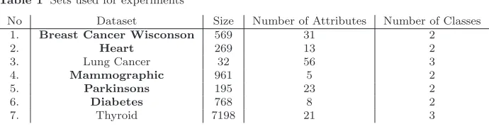
As can be seen in Table 1, these sets vary in terms of number of instances (from 32 to 7000 instances), number of attributes (from 5 to 56 attributes) and number of class labels (i.e. 2 and 3 classes). Notice that the data sets highlighted in boldfont in Table 1 have been used to apply single-class de-composition. In other words, for comparision purposes between our method
Table 1 Sets used for experiments
No Dataset Size Number of Attributes Number of Classes 1. Breast Cancer Wisconson 569 31 2
2. Heart 269 13 2
3. Lung Cancer 32 56 3
4. Mammographic 961 5 2
5. Parkinsons 195 23 2
6. Diabetes 768 8 2
7. Thyroid 7198 21 3
and the single class decomposition, we held the settings of all parameters the same, and the only change is related to the chosen data sets, where only those with binary classes have been considered.
4.2 Experiments Setup
In this subsection, we will use an illustrative example of running our method on the widely used Optical Recognition Character set (OCR) dataset from the UCI repository [5]. This illustration serves two purposes: (1) establishing the generality of the method for applying it to other domains; and (2) exem-plifying the methodology used in the evaluation when applied in the medical diagnosis domain. The feature set of every datasetAused in this experiment was subject to pre-processing where appropriate, in particular normalisation where features values are standardised in the range of 0 to 1 as can be seen in Equation6
zi=
xi−min(x)
max(x)−min(x) (6)
Where xi represents the ith value of feature/ attributex in the dataset,
andmax(x), min(x) represent the maximum and minimum values in feature
x. This step is important in particular to supress the sensitivity of kmeans
algorithms to outliers. Once data is normalised thenkmeansclustering algo-rithm was applied to it (Equation7), resulting in a new set with its class labels decomposed into a set of sub-classesk.
A′ =normalize(A) +cluster(A) (7)
For each dataset, Random Forest was applied to it twice. One time on the original data set (i.e. setA in Equation7) and we refer to this experiment as
9 5 .6 9 5 .8 9 6 .0
Number of Trees (K=3, Training Size=13212, Testing Size=6788)
C la ssi fi ca ti o n A ccu ra cy %
100 200 300 400 500 600 700 800 900 1000
RFC RF 9 5 .6 9 5 .8 9 6 .0
Number of Trees (K=4, Training Size=13212, Testing Size=6788)
C la ssi fi ca ti o n A ccu ra cy %
100 200 300 400 500 600 700 800 900 1000
RFC RF 9 5 .6 9 5 .9 9 6 .2
Number of Trees (K=5, Training Size=13212, Testing Size=6788)
C la ssi fi ca ti o n A ccu ra cy %
100 200 300 400 500 600 700 800 900 1000
RFC RF 9 5 .6 9 5 .8 9 6 .0 9 6 .2
Number of Trees (K=6, Training Size=13212, Testing Size=6788)
C la ssi fi ca ti o n A ccu ra cy %
100 200 300 400 500 600 700 800 900 1000
RFC RF 9 5 .6 9 5 .9 9 6 .2
Number of Trees (K=7, Training Size=13212, Testing Size=6788)
C la ssi fi ca ti o n A ccu ra cy %
100 200 300 400 500 600 700 800 900 1000
RFC RF 9 5 .6 9 5 .8 9 6 .0 9 6 .2
Number of Trees (K=8, Training Size=13212, Testing Size=6788)
C la ssi fi ca ti o n A ccu ra cy %
100 200 300 400 500 600 700 800 900 1000
RFC RF
Fig. 1 Experiment setup, single run
We used hold-out method in evaluating the predictive accuracy of the method. As can be seen in Figure 1, the size of the training set is almost 66% of the total size of the set (20,000), and each observation in the set has 16 attribute. It can be observed that our method (RF C) is winning in all set-tings over (RF) according to Figure1. The improvement in this experiment is statistically significant; adopting the pairedt-test, thep -valueis 6.932×10⁻⁷
with 95% confidence, and using the Wilcoxon signed rank test [33], thep-value 0.005889.
This experiment is given for illustration purposes, and thus we have only used one run. To ensure consistency of the results when applied on the medi-cal diagnosis datasets, each experiment was repeated 10 times, averaging the results.
4.3 Implementation & Working Environment
within the splits (i.e. training, testing). A typical result of one experimental run is shown in Table2. Notice here, that the best performing Random Forests results are selected (i.e. the ones with the best k values and the number of trees).
Table 2 Results of one experiment´s run (multi-class decomposition)
No Dataset Bestkvalues RF C RF Win-Lose
1. Breast Cancer Wisconson 3 93.78 93.78 Tie
2. Heart 3 82.42 84.62 Lose
3. Lung Cancer 1 70 70 Tie
4. Mammographic 3 85.58 84.97 Win
5. Parkinsons 3 93.94 90.91 Win
6. Diabetes 2 75.86 74.71 Win
7. Thyroid 3 99.55 99.51 Win
A computational framework was implemented using Rand randomForest package [22] which implements Brieman and Cutler Random Forest for Classi-fication and Regression2
. The experiment was carried out using Mac machine (OS X) with 16 GB of RAM and 2.6 GHz Intel Core i7. For both multi-class and single class decomposition we set the minimum kvalue to equal 2, while the maximum is set to equal 8. For the Lung cancer data set, we set kvalue to vary between 1 and 2, due to the very small size of the set. Notice that when k equals one then, bothRF and our method RF C must result in the same classification accuracy as can be seen in Table2. The maximumkvalue was set to equal 8 for these sets, because it turned out – experimentally – that increasing the value beyond this number does not improve the performance of our method. In [26], it was found that only 2 or 3 clusters for the positive class decomposition in a number of biomedical datasets are able to produce highest possible separable clusters. For validation purposes, we increased this number to 8. However, our study is consistent with the results reported in [26] that found only 2 or 3 clusters are adequate for biomedical datasets, and that clustering withk equals 4 through 10 yielded less separable clusters (in the case of multi-class decomposition). It is worth mentioning that diversity created by clusters is an important motive behind our method, and hence we experimented with up to 8 clusters.
4.4 Results & Discussion
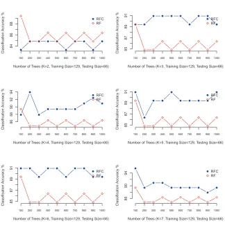
A single run over the datasets according to the above framework shows clearly that re-engineering the class labels improves the Random Forest performance as shown in Figure1 and as can be clearly seen in Figure2.
8 4 8 6 8 8
Number of Trees (K=2, Training Size=129, Testing Size=66)
C la ssi fi ca ti o n A ccu ra cy %
100 200 300 400 500 600 700 800 900 1000
RFC RF 8 5 8 7 8 9 9 1
Number of Trees (K=3, Training Size=129, Testing Size=66)
C la ssi fi ca ti o n A ccu ra cy %
100 200 300 400 500 600 700 800 900 1000
RFC RF 8 6 8 8 9 0 9 2 9 4
Number of Trees (K=4, Training Size=129, Testing Size=66)
C la ssi fi ca ti o n A ccu ra cy %
100 200 300 400 500 600 700 800 900 1000
RFC RF 8 5 8 7 8 9 9 1
Number of Trees (K=5, Training Size=129, Testing Size=66)
C la ssi fi ca ti o n A ccu ra cy %
100 200 300 400 500 600 700 800 900 1000
RFC RF 8 5 8 7 8 9 9 1
Number of Trees (K=6, Training Size=129, Testing Size=66)
C la ssi fi ca ti o n A ccu ra cy %
100 200 300 400 500 600 700 800 900 1000
RFC RF 8 6 9 0 9 4
Number of Trees (K=7, Training Size=129, Testing Size=66)
C la ssi fi ca ti o n A ccu ra cy %
100 200 300 400 500 600 700 800 900 1000
RFC RF
Fig. 2 Parkinsons Dataset, single run
As mentioned earlier, in order to ensure consistency of the results, the experiment was repeated 10 times for each set, and the results were averaged. Here, we also compare our approach to Random Forest and to AdaBoost. Table3summarises the results for all medical sets used in this paper.
Table 3 Average results of 10 runs, multi-class decomposition
No Dataset Size kvalues RF Cavg RFavg AdaBoostavg
1. Breast Cancer Wisconson 596 2to7 96.735 95.957 88.238
2. Heart 269 2to7 82.637 82.089 84.066
3. Lung Cancer 32 1to 2 68.956 66.737 63.000
4. Mammographic 961 2to7 83.835 83.181 82.147
5. Parkinsons 195 2to7 94.998 91.363 90.154
6. Diabetes 768 2to7 78.198 77.931 71.072
RF Cavg represents the results based on our method, while RFavg
repre-sents classical Random Forest (i.e. without class decomposition), andAdaBoostavg
represents the AdaBoost method. The results shown in Table3shows clearly that re-engineering class labels improves the performance of Random Forests. The improvement has an appropriate statistical significance for the application domain; adopting the pairedt-test, thep-value is 0.06189 with 95% confidence, and for the Wilcoxon signed rank test, thep-value = 0.03125. It is important to note here, that these results have been achieved with minimum parameter tuning. Thus, there is a clear potential for even further improvement. It is also clear from Table3that our proposed method outperformed the evidenced highly accurate ensemble classifier (AdaBoost). These results are also statisti-cally significant, adopting the paired t−test, thep-value is 0.03427 with 95% confidence, and the Wilcoxon signed rank test yielded ap-value of 0.04688.
A unique feature for our method is its applicability to multi-class problems, as discussed earlier in the paper. Thus, for the special case of binary classifica-tion problems, we run a set of experiments using the 5 binary datasets we use in this experimental work to compare the predictive accuracy of our technique to the previously proposed method by [26] to perform class decomposition on the positive class only. To ensure consistency, we used the same experimen-tal setup which includes repeating the experiment 10 times for each set, and then averaging the results. Table 4shows the superiority of our method (de-noted byRF Cavg) over the single-class decomposition method (RF CSavg) in
3 out of the 5 datasets. Paired t-test with 95% confidence revealed that the results are of minor statistical significance with p-value = 0.6298, and using the Wilcoxon signed rank test, thep-value = 0.625. Class decomposition over the positive class has helped improve the performance, as previously reported in [26]. However, it is worth noting that our method is more generic in terms to its applicability to all classification problems, and thus the results prove the potential of the new technique.
Table 4 Average results of 10 runs and comparision with the proposed method No Dataset # of Classes RF Cavg RF CSavg Difference
1 Breast Cancer Wisconson 2 96.73 96.27 +0.47
2 Heart 2 82.64 84.07 -1.43
3 Mammography 2 83.83 82.85 +0.98
4 Parkinsons 2 95.00 95.23 -0.23
5 Diabetes 2 78.20 76.63 +1.57
level of labelling, inherent subclasses can be always discovered at later stage. This is especially true in the medical domain. In recent years, a number of flu viruses have been affecting the world of travel and business. Modelling flu in a binary classifier that predicts the existence of one of the viruses can be achieved. However, precision can be enhanced, if class decomposition of the flu is applied, resulting in a multi-class problem. Finally, medical diagnosis is a complex process with a high degree of uncertainty and non-linearity, a class-decomposed data can simplify the process by looking at cohesive subclasses, instead of modelling more complex higher granular set of classes.
5 Conclusion & Future Work
This paper proposed adopting class decomposition using clustering instances that belong to the same label separately. The outcome of these clustering processes is a fine grained labelled dataset, that ultimately diversifies among individual trees in the trained Random Forests. Naturally, medical diagnosis datasets can further benefit from clustering by grouping the instances sharing similar feature values in one subclass (cluster). The proposed technique has been validated experimentally over 7 medical datasets, showing its potential in enhancing the predictive accuracy of Random Forests in medical diagnosis. We can indicate a number of future directions to further enhance the per-formance of the proposed method. Optimising the number of clusters per class can further enhance the performance. Some classes are in need to fine-grained decomposition where the number of clusters can be high; where some others may not need any class decomposition. The nature of the dataset can deter-mine whether or not clustering is needed and the optimum number of clusters. This can be objectively measured using one of the cluster quality measures (e.g., DBI [20]). Also other clustering techniques can be used instead of k -means.
Another direction of future work is to investigate cluster proximity among different classes when classifying unseen instance. Currently, if an instance is assigned to a cluster that belongs to one class, it is assigned the label of the parent class. However, there is a possibility of having a cluster that has proximity to other classes. This is especially true in medical datasets, when symptoms of the different diseases have high degree of similarity.
Finally, as the proposed technique converts binary classification problems to multi-class ones, Error COrrecting Code (ECOC) ensemble methods [9] can be applied to further diversify the classification from the output side. This is especially interesting investigation, as artificial classes (clusters) can enrich possible combination of binary classification problems for the ECOC.
References
IEEE Symposium on, pages 283–290. IEEE, 2011.
2. Z. S. Abdallah, M. M. Gaber, B. Srinivasan, and S. Krishnaswamy. Adaptive mobile activity recognition system with evolving data streams. Neurocomputing, 150:304–317, 2015.
3. D. Amaratunga, J. Cabrera, and Y.-S. Lee. Enriched random forests. Bioinformatics, 24(18):2010–2014, 2008.
4. Y. Amit and D. Geman. Shape quantization and recognition with randomized trees. Neural Comput., 9(7):1545–1588, Oct. 1997.
5. K. Bache and M. Lichman. UCI machine learning repository, 2013.
6. M. Bader-El-Den and M. Gaber. Garf: towards self-optimised random forests. InNeural Information Processing, pages 506–515. Springer, 2012.
7. L. Breiman. Bagging predictors. Mach. Learn., 24(2):123–140, Aug. 1996. 8. L. Breiman. Random forests.Mach. Learn., 45(1):5–32, Oct. 2001.
9. T. G. Dietterich and G. Bakiri. Error-correcting output codes: A general method for improving multiclass inductive learning programs. InAAAI, pages 572–577. Citeseer, 1991.
10. H. Drucker, C. Cortes, L. D. Jackel, Y. LeCun, and V. Vapnik. Boosting and other ensemble methods.Neural Computation, 6(6):1289–1301, 1994.
11. M. Elter, R. Schulz-Wendtland, and T. Wittenberg. The prediction of breast cancer biopsy outcomes using two CAD approaches that both emphasize an intelligible decision process.Medical Physics, 34:4164, 2007.
12. K. Fawagreh, M. M. Gaber, and E. Elyan. Diversified random forests using random subspaces. In Intelligent Data Engineering and Automated Learning–IDEAL 2014, pages 85–92. Springer, 2014.
13. K. Fawagreh, M. M. Gaber, and E. Elyan. Random forests: from early developments to recent advancements. Systems Science & Control Engineering: An Open Access Journal, 2(1):602–609, 2014.
14. M. Fern´andez-Delgado, E. Cernadas, S. Barro, and D. Amorim. Do we need hundreds of classifiers to solve real world classification problems? Journal of Machine Learning Research, 15:3133–3181, 2014.
15. Y. Freund. Boosting a weak learning algorithm by majority. Information and compu-tation, 121(2):256–285, 1995.
16. J. H. Friedman. Stochastic gradient boosting. Computational Statistics & Data Anal-ysis, 38(4):367–378, 2002.
17. T. K. Ho. Random decision forests. InDocument Analysis and Recognition, 1995., Proceedings of the Third International Conference on, volume 1, pages 278–282 vol.1, Aug 1995.
18. T. K. Ho. The random subspace method for constructing decision forests. Pattern Analysis and Machine Intelligence, IEEE Transactions on, 20(8):832–844, Aug 1998. 19. Z.-Q. Hong and J.-Y. Yang. Optimal discriminant plane for a small number of samples
and design method of classifier on the plane.Pattern Recognition, 24(4):317 – 324, 1991. 20. A. K. Jain, R. C. Dubes, et al. Algorithms for clustering data, volume 6. Prentice hall
Englewood Cliffs, 1988.
21. P. Latinne, O. Debeir, and C. Decaestecker. Limiting the number of trees in random forests. InMultiple Classifier Systems, pages 178–187. Springer, 2001.
22. A. Liaw and M. Wiener. Classification and regression by randomforest.R News, 2(3):18– 22, 2002.
23. M. Little, P. McSharry, S. Roberts, D. Costello, and I. Moroz. Exploiting nonlinear recurrence and fractal scaling properties for voice disorder detection.BioMedical Engi-neering OnLine, 6(1), 2007.
24. J. MacQueen. Some methods for classification and analysis of multivariate observations, 1967.
25. O. L. Mangasarian, W. N. Street, and W. H. Wolberg. Breast cancer diagnosis and prognosis via linear programming.OPERATIONS RESEARCH, 43:570–577, 1995. 26. I. Polaka. Clustering algorithm specifics in class decomposition. No: Applied
Informa-tion and CommunicaInforma-tion Technology, 2013.
28. U. Repository. Heart Disease dataset. https://archive.ics.uci.edu/ml/datasets/ Statlog+(Heart), 1996. [Online; accessed Dec-2014].
29. M. Robnik-ˇSikonja. Improving random forests. In Machine Learning: ECML 2004, pages 359–370. Springer, 2004.
30. A. Tsymbal, M. Pechenizkiy, and P. Cunningham. Dynamic integration with random forests. InMachine Learning: ECML 2006, pages 801–808. Springer, 2006.
31. R. Vilalta, M.-K. Achari, and C. F. Eick. Class decomposition via clustering: a new framework for low-variance classifiers. InData Mining, 2003. ICDM 2003. Third IEEE International Conference on, pages 673–676. IEEE, 2003.
32. D. H. Wolpert. Stacked generalization.Neural networks, 5(2):241–259, 1992. 33. R. Woolson. Wilcoxon signed-rank test. Wiley Encyclopedia of Clinical Trials, 2008.