Explicit and Exact Traveling Wave Solutions of Cahn Allen Equation Using MSE Method

Article

Explicit and Exact Traveling Wave Solutions of the

Cahn–Allen Equation Using the MSE Method

Harun-Or-Roshid1,*, M. Zulfikar Ali2 and Md. Rafiqul Islam1,*

1 _{Department of Mathematics, Pabna University of Science and Technology, Pabna-6600, Bangladesh} 2 _{Department of Mathematics, Rajshahi University, Rajshahi-1206, Bangladesh; [email protected]}

* Correspondence: [email protected] (H.-O.-R.);[email protected] (M.R.I.); Tel.: +88-01754-213-813

Abstract: By using the modified simple equation method, we study the Cahn–Allen equation, which arises in many scientific applications such as mathematical biology, quantum mechanics, and plasma physics. As a result, the existence of solitary wave solutions of the Cahn–Allen equation is obtained. Exact explicit solutions interms of hyperbolic solutions of the associated Cahn–Allen equation are characterized with some free parameters. Finally, the variety of structures and graphical representations make the dynamics of the equations visible and provide the mathematical foundation in mathematical biology, quantum mechanics and plasma physics.

Keywords: the modified simple equation method; Cahn–Allen equation; soliton solution; kink type solutions

1. Introduction

The mathematical modeling of events in nature can be explained by differential equations.It is well-known that various types of the physical phenomena in the fieldsof fluid mechanics, quantummechanics, electricity, plasma physics, chemical kinematics,propagation of shallow water waves and optical fibers aremodeled by nonlinear evolution equations, and the appearanceof solitary wave solutions in nature is somewhat frequent.However, the nonlinear process is one of the major challengesand not easy to control because the nonlinear characteristicsof the system abruptly change due to some small changes in parameters including time. Thus, this issue becomes moredifficult and hence a crucial solution is needed. The solutions of these equations have crucial impact in mathematical physics and engineering. The variety of solutions of NLEEs, which are mutual different operating mathematical techniques, is very important in many fields of science such as fluid mechanics, optical fibers, technology of space, control engineering problems, hydrodynamics, meteorology, plasma physics, applied mathematics. Advanced nonlinear techniques are importantfor solving inherentnonlinear problems, particularly those involving dynamicalsystems and allied areas. In recent years, there have beenbigimprovements in finding the exact solutions of NLEEs.Many powerful methods have been establishedand enhanced, such as the modified extended Fan sub-equation method [1], the homogeneous balance method [2,3], the Jacobi elliptic function expansion [4], the Backlund transformation method [5,6], the Darboux transformation method [7],the Adomian decomposition method [8–9], the auxiliary equation method[10,11], the (G′/G)-expansion method [12–18], the Exp-(−φ ξ( ))-expansion method [19], the sine-cosine method [20–22], the tanh method [23],the F-expansion method [24,25], the exp-function method [26,27],the modified simple equation method [28–30],the first integral method [31], the simple equation method [32], the bilinear method[33], the transformed rational function method[34],and so on. Most of the above methods are dependent on computational software except the MSE method.

2. Description of the MSE Method

Consider a general form of a nonlinear evolution equation,

( , , , , ,

_{t x xt xx}

) 0

H u u u u u

 

=

, (1)

whereu( )ξ =u x t( , ) is an unknown function,

H

is a polynomial of u x t( , ) and its partial derivatives in which the highest order derivatives and nonlinear terms are involved. In the following,we present the main steps of the method:

Step 1:Combine the real variables

x

and

t

by acompound variableξ_:

( , ) ( )

u r t = ξu ,

ξ=

P r wt

.

±

_. (2)

Here,

P li mj nk

= + +

ˆ

ˆ

ˆ

and

P xi yj zk

= + +

ˆ

ˆ

ˆ

where l m n, , are the constant magnitudes along the axes of

x y z

, ,

respectively,

μ

is wave number and

w

is the speed of the traveling wave.

This travelling wave transformation permits us to reduce Equation (1) to the following ordinary differential equation (ODE):

( , , ) 0

G u u u′ ′′   =

,

₍₃₎

where

G

is a polynomial in u( )ξ and its derivatives, wherein

2

2

( )

du

, ( )

d u

u

u

d

d

′

ξ =

′′

ξ =

ξ

ξ

and so on.

Step 2: We also consider that the Equation (3) has the formal solution:

0

( ) ( )

( )

i n

i i

S

u A

S

=

′

 _ξ 

ξ =  

ξ

 



,

(4)

where

A

_i

(0

≤ ≤

i n

)

are constants to be determined, andS( )ξ is also unknown function to be evaluated.

Step 3: The value of positive integer n in Equation (4) can be determined by taking into account the homogeneous balance between the highest order nonlinear terms and the derivatives of highest order occurring in Equation (3). If the degree of u( )ξ isD u( ( ))ξ =n_{,then the degree of the other}

expression will be u( )ξ as follows:

( )

p p

d u

D

n

p

d



ξ = +





ξ







,

( )

(

)

s q p

q

d u

D u

np s n q

d





ξ













=

+

+





ξ









.

Step 4:Inserting Equation (4) into Equation (3), we get a polynomial of( ( ) / ( ))S′ ξ S ξ and its derivatives and ( ( )) , (S ξ −i i=0,1, 2,, )n . In the resultant polynomial, we equate all the coefficients of( ( )) , (S ξ −i i=0,1, 2,, )n to zero. This technique produces a system of algebraic and differential equations that can be solved receiving A i_i( =0,1, 2,, ),n S( )ξ and the value of the other needful parameters.This completes the determination of the solution to the Equation (1).

Remark.In comparison,in the modified simple equation method with the simple equation method [32], it is seen that the simple equation method gets help froman auxiliary equation (the Riccati equation), but the modified simple equation method can perform directly without help from an auxiliary equation. On the other hand, the simple equation method yields results that are a special case from the modified equation method.

3. Traveling Wave Solution of the Cahn–Allen Equation

m

t xx

u u

= − +

u

u

;

(5)

for

m

=

3

,Equation (5) becomes the Cahn–Allen equation [29,30]. This equation arises in many scientific applications such as mathematical biology, quantum mechanics and plasma physics. To solvethis example, we can use transformation ξ = kx+w t (where

k

and

w

are the wave number andthe wave speed, respectively), and then Equation (5) becomes ordinary differential equation:

2 3 ₀

wu′−k u′′+u − =u

.

(6)

Balancing u3with

u

′′

then gives

n

=

1

:

0 1

( )

( )

( )

S

u

A A

S

′ ξ

ξ = +

ξ

.

(7)

2

1 1

( ) ( )

( )

( ) ( )

S S

u A A

S S

′′ _ξ  ′ _ξ 

′ ξ = _ξ −  _ξ 

  _. (8)

3

1 1 2 1

( ) ( ) ( ) ( )

( ) 3 2

( ) ( ) ( )

S S S S

u A A A

S S S

′′′_ξ ′′ _ξ ′ _ξ  ′ _ξ 

′′ ξ = − +  

ξ ξ  ξ  _. (9)

Putting Equations (6)–(9) in Equation (6) and equating coefficients of like powers of

( )

( )

S

S

′ ξ

ξ

, we get:

Coefficient of

(

S

( ) :

ξ

)

0

3

0 0

0

A A

− =

; (10)

Coefficient of

(

S

( )

ξ

)

−1

:

2 2

1

( ) 3

0 1

( )

1

( )

1

( ) 0

k AS

′′′

A AS

′

wAS

′′

AS

′

−

ξ +

ξ +

ξ −

ξ =

_; (11)

Coefficient of

(

)

2

( )

:

S

ξ

−

(

)

2 _{3 2}

(

)

2

1

( )

3

1

( ) ( ) 3

0 1

( )

0

wA S

′

k A S

′

S

′′

A A S

′

−

ξ

+

ξ

ξ +

ξ

=

(12)

and Coefficient of

(

)

3

( )

:

S

ξ

−

(

)

3

2 2

1

(

1

2 )

( )

0

A A

−

k

S

′

ξ

=

_. (13)

From Equation(10), we achieve

A

₀

=

0,1, 1

−

and from Equation(13),

A

₁

≠

0

thus

A

₁

= ±

2

k

,

2 2

0 0 1

2

0 1

3 (3

1)

(

3

)

(

3

)

k

A

w w

A A

S

S

k w

A A

′′′

=

− +

−

′′

−

.

(14)

2 2

0 0 1

1 2

0 1

3 (3

1)

(

3

)

exp(

)

(

3

)

k

A

w w

A A

S

c

k w

A A

− +

−

′′ =

ξ

−

.

(15)

From Equation (12),

2 2

2

0 0 1

1

2

0 1 0 1

3 (3

1)

(

3

)

3

exp(

)

3

(

3

)

k

A

w w

A A

c k

S

w

A A

k w

A A

− +

−

′ =

ξ

−

−

(16)

and

2 2

4

0 0 1

1

2

2 2 2

0 0 1 0 1

3 (3

1)

(

3

)

3

exp(

)

3 (3

1)

(

3

)

(

3

)

k

A

w w

A A

c k

S

c

k

A

w w

A A

k w

A A

− +

−

=

ξ +

− +

−

−

_. (17)

Using Equations (16) and (17), we attain

2 2

0 0 1

2 2

0 1 1 1

0 4 2 2

0 0 1

1 0 1

2

2 2 2

0 0 1 0 1

3 (3 1) ( 3 )

exp( )

( 3 )

3

3 (3 1) ( 3 )

3 3

exp( )

3 (3 1) ( 3 ) ( 3 )

k A w w A A

k w A A

c A k

u A

k A w w A A

c k

w A A

c

k A w w A A k w A A

− + − _ξ − = + × − + − − _{ξ +} − + − −

,

(18)

where

(

3

)

2

k x

t

ξ =

±

with

3

2

w

= ±

k

. Here,

c

₁ and

c

₂ are arbitrary constants.

Case-I:For set

A

₀

=

0,

A

₁

= ±

2

k

, we get

2 2

3 2

1

4 2 2

1

2

2 2 2

3 )

exp(

)

3 2

)

3

3 )

exp(

)

3

)

w

k

c k

k w

u

c k

w

k

w

c

w

k

k w

−

ξ

= ±

×

−

ξ +

−

,

(19) where 3 ( ) 2

k x t ξ = ±

with

3 2

w= ± k

.

If

4 1 2 2 2

3

3

k c

c

w

k

=

−

,then

2 2 2 2

2

3

3

1 tanh

2

2

w

k

w

k

u

wk

wk









−



−



= ±



+



ξ

















,

(20)

where

3

(

)

2

k x

t

ξ =

±

, with

3

2

w

= ±

k

.

If

4 1

2 2 2

3

3

k c

c

w

k

= −

−

,then

2 2 2 2

2

3

3

1 coth

2

2

w

k

w

k

u

wk

wk









−



−



= ±



+



ξ

















_, (21)

where

3

(

)

2

k x

t

ξ =

±

Since

c

₁ and

c

₂ are arbitrary constants, for other choices of

c

₁ and

c

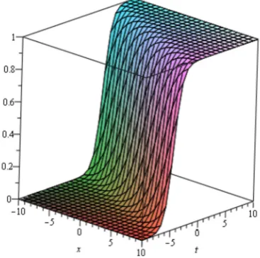
₂

, it might yield many new and more general exact solutions of the nonlinear Cahn–Allen equation withoutany aid of symbolic computation software.The solutions u(x,t) obtained in Equations (20) and (21) arepresented in the following figures: (see Figures 1 and 2).

Figure 1. Kink wave of Equation (20) with

k

=

1

.

Figure 2. Single soliton solution of Equation(21) with

k

=

1

.

Case-II:For set

A

₀

= ±

1,

A

₁

= ±

2

k

, we get

2

3 2

1

4 2

1

2

2 2

6

(

3 2 ))

exp(

)

3 2

(

3 2 )

1

3

3 2

6

(

3 2 ))

exp(

)

6

(

3 2 )

(

3 2 )

k

w w

k

c k

k w

k

u

c k

w

k

k

w w

k

c

k

w w

k

k w

k

+

−

ξ

−

= ± ±

×

−

+

−

ξ +

+

−

−

,

(22)

where

(

3

)

2

k x

t

ξ =

±

with

3

2

w

= ±

k

. Here,

c

₁ and

c

₂ are arbitrary constants.

If

4 1

2 ₂

3

6

(

3 2 )

k c

c

k

w w

k

=

2 2

2

2{6

(

3 2 )}

6

(

3 2 ))

1

1 tanh

(

3 2 )

(

3 2 )

k

w w

k

k

w w

k

u

k w

k

k w

k









+

−



+

−



= ± ±



+





ξ







−







−







,

(23)

where

3

(

)

2

k x

t

ξ =

±

, with

3

2

w

= ±

k

.

If

4 1

2 ₂

3

6

(

3 2 )

k c

c

k

w w

k

= −

+

−

_,then

2 2

2

2{6

(

3 2 )}

6

(

3 2 ))

1

1 tanh

(

3 2 )

(

3 2 )

k

w w

k

k

w w

k

u

k w

k

k w

k









+

−



+

−



= ± ±



+





ξ







−







−







,

(24)

where

3

(

)

2

k x

t

ξ =

±

, with

3

2

w

= ±

k

.

Since

c

1 and

c

2 are arbitrary constants, for other choices of

c

1 and

c

2_, it might yield many

new and more general exact solutions of the nonlinear Cahn–Allen equation withoutany aid of symbolic computation software.

The solutions u x t( , ) obtained in Equation(23)are similar to Figure 1, and Equation (24) is similar to Figure2 and omitted for convenience.

Again with commercial software, we can find some solutions of the Cahn–Allen equation (solving fromEquations (11) and (12)).

For

A

₀

=

0,

A

₁

= ±

2

k

,we get

S

( )

ξ = +

a b

exp(

±ξ

/ 2 )

k

. And thus,

( , )

cosh

sinh

2

2

b

u x t

a

b

k

k

= ±

ξ

ξ





+











with ξ =k x

(

±3 / 2t

)

. (25)

If we consider a b/ =exp(2 )c _{, then Equation(25) reduces to well known solution:}

1

1

3

( , )

1 tanh

2

2

2

u x t

= ±





+





±

x

+

t c

+

















_. (26)

For

A

₀

=

1,

A

₁

= ±

2

k

,we get

S

( )

ξ = +

a b

exp( / 2 )

±ξ

k

, and thus,

( , ) 1

cosh

sinh

2

2

b

u x t

a

b

k

k

= −

ξ

ξ





±

+









with ξ =k x

(

±3 / 2t

)

. (27)

If we consider a b/ =exp(2 )c _{, then Equation(26) reduces to well known solution:}

1

1

3

( , )

1 tanh

2

2

2

u x t

=





+







±

x

+

t c

+















_. (28)

For

A

₀

= −

1,

A

₁

= ±

2

k

and thus,

( , )

1

cosh

sinh

2

2

b

u x t

a

b

k

k

= − −

ξ

ξ





+











with ξ =k x

(

3 / 2t

)

. (29)

If we consider a b/ =exp(2 )c _{,then Equation(26) reduces to well known solution:}

1

1

3

( , )

1 tanh

2

2

2

u x t

= −





+







±

x

+

t c

+















_. (30)

Since a and b are arbitrary constants, for other choices of a and

b

_{, it might yield many new} and more general exact solutions of the nonlinear Cahn–Allen equation. When we choose

/ exp(2 )

a b= c _{,we get special type solutions like Equations (28) and (30), but if we choose} a and b

in different ways, we can get different types of solutions. Thus,Equations (28) and (30) are special types of our solutions.

Graphs of Equations (25), (27) and (29) represent kink type like Figure 1 both for positive/negative values of the arbitrary constants c1 and c2like single solitons such as Figure 2

fortheir opposite values.

4. Comparison

In this section, we compare our solution with some well-known methods, namely the exp-function method and the first integral method as follows:

(a) Comparison with Exp-method Reference [27]:Ugurlu [27] obtained some solutions of the Cahn–Allen equation via the exp-function method,in which solutions u u8, 9 are identical with

Equation (25) when b=1,a =b0_, and the other solutions are different from their solutions(for

more, see Ref. [27]).

(b)Comparison with First Integral method Reference [31]:Tascan and Bekir [31] obtained some solutions of the Cahn–Allen equation via the first integral method, in which Equation(3.20) is identical with Equation (25) (when, in our study,a = =b 1,k = −1 / 2_{,and, in their study,}

c

₀

=

0

)

8

,

9

u u

is identical with Equation (25) when

b

=

1,

a b

=

0_, and the other solutions are different from

their solutions. On the contrary, by using theMSE method in this article, we obtained four solutions withless calculations.

5. Conclusions

In this article, we have successfully implemented the MSE method to find the exact traveling wave solutions of the Cahn–Allen equation. Comparing the MSE method to other methods, we claim that the MSE method is straight forward, efficient, and can be used in many other nonlinear evolution equations. In the existing methods, such as the (G’/G)-expansion method, the exp-function method, and the tanh-function method, it is requires making use of symbolic computation software, such as Mathematica or Maple-13 to facilitate complex algebraic computations. To solve non-linear evolution equations via the MSE method, no auxiliary equations are needed. On the other hand, via the MSE method, the exact and solitary wave solutions to these equations have been achieved without using any symbolic computation software because the method is very simple and has easy computations.

Author Contributions: HOR proposed the algorithm. MZA developed, analyzed and implement the methods. MRI contributed to the implementation of the methods. All authors approved the final manuscript.

Conflicts of Interest: The authors declare that they have no competing interests.

References

1. Yomba, E.The modified extended Fan sub-equation method and its application to the (2+1)-Dimensional

Broer-Kaup-Kuperschmidt equations. Chaos Solitons Fractals2006, 27, 187–196.

2. Zayed, E.M.E.; Zedan, H.A.; Gepreel, K.A. On the solitary wave solutions for nonlinear Hirota-Sasuma

coupled KDV equations. Chaos Solitons Fractals2004, 22, 285–303.

3. Wang, M.L. Exact solutions for a compound KdV-Burgers equation.Phys. Lett.A1996, 213, 279–287.

4. Yan, Z. Abundant families of Jacobi elliptic function solutions of the (G’/G)-dimensional integrable

Davey-Stewartson- type equation via a new method.Chaos Solitons Fractals2003, 18, 299–309. 5. Miura, M.R.Backlund Transformation; Springer: Berlin, Germany,1978.

6. Ma, W.X.;Fuchssteiner, B. Explicit and exact solutions to a Kolmogorov-Petrovskii-Piskunov equation.Int.

J. Non-Linear Mech.1996, 31, 329–338.

7. Matveev, V.B.; Salle, M.A.Darboux Transformation and Solitons; Springer: Berlin, Germany, 1991.

8. Wu, T.Y.; Zhang, J.E.On Modeling Nonlinear Long Waves.In Mathematics Is for Solving Problems;Cook, P.,

Roytburd, V.,Tulin, M., Eds.; SIAM: Philadelphia, PA, USA, 1996; pp. 233–249.

9. Adomain, G.Solving Frontier Problems of Physics: The Decomposition Method; Kluwer Academic Publishers:

Boston, MA, USA, 1994.

10. Sirendaoreji; Sun, J. Auxiliary equation method for solving nonlinear partial differential equations. Phys.

Lett.A2003, 309, 387–396.

11. Sirendaoreji. Auxiliary equation method and new solutions of Klein-Gordon equations. Chaos Solitions

Fractals 2007, 31, 943–950.

12. Wang, M.L.; Li, X.Z.; Zhang, J. The (G′/G) -expansion method and traveling wave solutions of

nonlinear evolution equations in mathematical physics. Phys. Lett. A2008, 372, 417–423.

13. Bekir, A. Application of the (G′/G)-expansion method for nonlinear evolution equations.Phys. Lett.

A2008, 372, 3400–3406.

14. Roshid, H.O.; Hoque, M.F.; Akbar, M.A. New extended (G′/G)-expansion method for traveling wave

solutions of nonlinear partial differential equations (NPDEs) in mathematical physics. Ital. J. PureAppl.

Math.2014, 33, 175–190.

15. Roshid, H.O.; Alam, M.N.; Hoque, M.F.; Akbar, M.A. A new extended (G′/G)-expansion method to

find exact traveling wave solutions of nonlinear evolution equations. Math. Stat.2013, 1, 2013 162–166. 16. Neyrame, A.; Roozi, A.; Hosseini, S.S.; Shafiof, S.M. Exact travelling wave solutions for some nonlinear

partial differential equations.J. King Saud Univ.-Sci.2012, 22, 275–278.

17. Roshid, H.O.; Rahman, N.; Akbar, M.A. Traveling wave solutions of nonlinear Klein-Gordon equation by extended (G′/G)-expansion method.Ann.Pure Appl. Math.2013, 3, 10–16.

18. Salehpour, E.; Jafari, H.; Kadkhoda, N. Application of (G’/G)-expansion Method to Nonlinear Lienard

Equation. Indian J. Sci. Tech.2012, 5, 2454–2456.

19. Roshid, H.O.; Rahman, M.A. The exp(−Φ η( )) -expansion method with application in the

20. Wazwaz, A.M.Exact solutions of compact and noncompact structures for the KP–BBM equation.Appl.

Math. Comput.2005, 169, 700–712.

21. Wazwaz, A.M.Compact and noncompact physical structures forthe ZK-BBM equation.Appl.

Math.Compact.2005, 169, 713–725.

22. Wazwaz, A.M.The sine-cosine method for obtaining solutions with compact and noncompact structures.

Appl. Math. Comput.2004, 159, 559–576.

23. Wazwaz, A.M. The extended tanh method for new compact and noncompact solutions for the KP-BBM

and the ZK-BBM equations.Chaos Solitons Fractals2008, 38, 1505–1516.

24. Abdou, M.A.The extended F-expansion method and its application for a class of nonlinearevolution

equations. Chaos Solitons Fractals2007, 31, 95–104.

25. Abdou, M.A.Exact periodicwave solutions to some nonlinear evolution equations. Int. J.Nonlinear Sci.2008, 6, 145–153.

26. Mahmoudi, J.; Tolou, N.; Khatami, I.; Barari, A.; Ganji, D.D.Explicit solution of nonlinear ZK-BBM wave

equation using Exp-function method. J. Appl. Sci.2008, 8, 358–363.

27. Ugurlu, Y. Exp-function method for the some nonlinear partial differential equations. Math. Aeterna2013, 3, 57–70.

28. Jawad, A.J.M.; Petkovic, M.D.; Biswas, A. Modified simple equation method for nonlinear evolution

equations. Appl. Math. Comput.2010, 217, 869–877.

29. Zayed, E.M.E. A note on the modified simple equation method applied to Sharma–Tasso–Olver equation.

Appl. Math. Comput.2011, 218, 3962–3964.

30. Zayed, E.M.E.; Ibrahim, S.A.H. Exact solutions of nonlinear evolution equations in mathematical physics

using the modified simple equation method. Chin. Phys. Lett.2012, 29, 060201.

31. Tascan, F.; Bekir, A. traveling wave solutions of the Cahn-Allen equation by using first integral method.

Appl. Math. Comput.2007, 207, 279–282.

32. Jafari, H.; Kadkhoda, N. Application of simplest equation method to the (2+ 1)-dimensional nonlinear

evolution equations.New Trends Math. Sci.2014, 2, 64–68.

33. Ma,W.X. Generalized Bilinear Differential Equations. Studies Nonlinear Sci.2011, 2, 140–144.

34. Ma, W.X.;Lee, J.H. A transformed rational function method and exact solutions to the 3+1 dimensional

Jimbo–Miwa equation.Chaos Solitons Fractals2009, 42, 1356–1363.