A Spark-based genetic algorithm for sensor placement in large
scale drinking water distribution systems
Chengyu Hu1 · Guo Ren1 · Chao Liu1 · Ming Li2 · Wei Jie3
Abstract Water pollution incidents have occurred fre-quently in recent years, causing severe damages, economic loss and long-lasting society impact. A viable solution is to install water quality monitoring sensors in water supply networks (WSNs) for real-time pollution detection, thereby mitigating the risk of catastrophic contamination incidents. Given the significant cost of placing sensors at all locations in a network, a critical issue is where to deploy sensors within WSNs, while achieving rapid detection of contam-inant events. Existing studies have mainly focused on sensor placement in water distribution systems (WDSs). However, the problem is still not adequately addressed, especially for large scale WSNs. In this paper, we investigate the sensor placement problem in large scale WDSs with the objective of minimizing the impact of contamination events. Specifi-cally, we propose a two-phase Spark-based genetic algorithm (SGA). Experimental results show that SGA outperforms
B
Chao Liu[email protected] Chengyu Hu
[email protected] Guo Ren
[email protected] Ming Li
[email protected] Wei Jie
1 School of Computer Science, China University of
Geosciences, Wuhan, China
2 Department of Computer Science, California State
University, Fresno, CA, USA
3 School of Computing and Engineering, University of West
London, London, UK
other traditional algorithms in both accuracy and efficiency, which validates the feasibility and effectiveness of our pro-posed approach.
Keywords Sensor placement·Water distribution system· Genetic algorithm·Spark
1 Introduction
Clean drinking water is a critical resource for the health and well-being of all humans. However, water quality can easily deteriorate because of malicious attack or accidental incident. For example, an outbreak of waterborne disease epidemic in Walkerton, Ontario, Canada, in 2000 affected 2,300 people as a result of exposure to contaminated drinking water [1]. An Event such as the poisoning of water supply caused 71 people poisoned happened in Ruyang city, Henan Province, China in 2007 [2].
Deploying water quality sensor networks is considered as a viable approach for detecting contamination incidents in drinking WDS [3,4]. However, high cost of water qual-ity sensors (e.g., a Hach chlorine sensor costs between USD 3000–5000) and installation/maintenance, as well as opti-mization methods, limit the number of sensor [5]. How to quickly detect the contaminant event in a large scale WDS with a fixed number of water quality sensors is a critical problem.
In the past decade, although SPP in drinking WDS has been well investigated, there are two main problems for deploying sensors in a large scale WSN (e.g., the number of node is greater than 10,000):
sensor-constrained optimization problem, i.e. allowing only a fixed number of sensors; the other is a time-constrained optimization problem, i. e. requiring con-tamination detection within a given time limit. Some researchers have proved that the two problems are NP-hard or NP-Complete [6], and the former is polynomially equivalent to the asymmetric k-center problem, the lat-ter is polynomially equivalent to the dominating set problem. Similarly, Carr et al. [7] formulated SPP as a mixed-integer program and proved that its complexity is NP-hard when the objective coefficients are not known with certainty.
– Large computation overhead. Drinking WDS in the real world is a complexity system which consists of thou-sands of miles of pipes, valves and pumps, which results in significant computational efforts for water quality sim-ulation. As an example WSN shown in the battle of the water sensor network has 12,523 nodes, 2 sources, 2 tanks, 14822 pipes, 4 pumps, 5 valves [8]. Large scale WSN results in expensive computation overhead and storage requirement. For a large scale network with about 10,000 nodes, if each node has a probability of being injected contaminant, with the sampling time of the sen-sor being 10 min and the whole simulation time being 72 h, then we need to simulate 10,000×72×60÷10 = 4.32 million contaminant scenarios. If we consider that storing the contaminant concentration at each node needs 4 byte for each scenario, then the requirement of storage is 172.8 Gigabytes. Considering the running time of sim-ulation on this network (roughly 4 s on a current Pentium 4.3GHz), the time for an exhaustive simulation of all 4.32 million scenarios would require roughly 200 days [9].
To deal with computational complexity of SPP, some researchers applied some rule-based or graph-based meth-ods to avoid the dilemma. For example, Chang et al. [10] employed two rules (e.g., accessibility and complexity rules) to generate a set of sensor placement locations. These meth-ods do not need to simulate hydraulic and quality transport model, therefore incurring little computation and storage overhead. However, these methods seem to be too crude to locate sensors because they generally do not take into account the transport process of drinking water in WSN. In fact, for NP-hard or NP-Complete problems, evolutionary algo-rithms are a set of competent methods to get a near-optimal or optimal solution [11,12]. However, evolutionary algorithms often lead to longer computation. A big challenge is how to quickly and efficiently generate a near-optimal solution.
In recent years, there are a few research works on WDS involved in high performance computation. SPP is dealt with by the combination of parallel processing technique and evolutionary computation. Laszewski et al. [13] solved the contaminant source identification (CSI) problem on the
super-computing resources of TeraGrid. Wu et al. [14] inves-tigated the use of cloud computing in WDSs, where a pump scheduler has been deployed onto the high performance com-puter, through which a user can submit, execute and retrieve optimization analysis jobs. Shen et al. [15] applied paral-lel computing to simulate intrusion events for CSI problem with a super-computer. Wang et al. [16] presented a parallel method for the first time using the MapReduce paradigm to identify the contamination source in WDS.
To the best of our knowledge, there is no method that has been proposed in literatures for SPP using Spark to paral-lelize genetic algorithm (GA). Herein, as a first attempt, we use Spark to implement two-phase genetic algorithm. The first phase is fitness evaluation parallelization, and the second phase is genetic operations. More specifically, the contribu-tions of our work are as follows:
– We present the system model and formulate SPP into a mixed-integer programming problem that satisfies the goal of minimizing the average time of detecting the con-taminant events.
– We propose a two-phase genetic algorithm based on Spark model for sensor placement in drinking WDS. – We give a comprehensive evaluation of the proposed
algorithm. Through experiments, we verify the perfor-mance and effectiveness of our proposed algorithm.
The rest of the paper is organized as follows. Section2 reviews the state of arts. Section3focuses on system model and mathematic formulation. Section4presents our proposed algorithm. Section5discusses simulation results. Section6 concludes the paper and puts forward some issues which need to be further investigated in the future.
2 Related work
Sensor placement is to deploy water quality sensor in WSN, with the purposes of protecting municipal people against both deliberate and accidental hazard‘s intrusions. The physical structure of a water distribution system is a network in which nodes represent water sources, tanks, and junctions.
Fig. 1 A WDS with 126 nodes, 1 source, 2 tanks, 168 pipes, 2 pumps and 8 valves
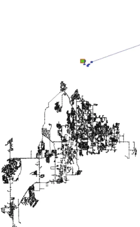
Fig. 2 Placement of Network2 in BWSN (12,523 nodes, 2 sources, 2 tanks, 14,822 pipes, 4 pumps, 5 valves) [8]
In Fig.1, we are mainly concerned with which node should be deployed with sensors. For a small or medium scale WSN, it is easy to give the optimal placement of sensors by exhaus-tive search. However, it is a difficult task to obtain the optimal sensor placement for a large scale WSN. As shown in the example of Fig.2, if we deploy 20 sensor to the WSN with 10,000 nodes, there areC1020,000 placement schemes of sen-sors.
2.1 Some approaches for sensor placement problem in WDS
For the SPP in WDS, a variety of different sensor place-ment optimization algorithms have been used to address the problem. They includes deterministic or heuristic algorithm, such as integer programming, genetic algorithm, simulated annealing and ant colony optimization [17].
As a high dimensional combination optimization prob-lem, SPP is too computationally-intensive to find an exact solution. However, sometimes a near-optimal solution can be sufficient. Therefore, some effective heuristic random algo-rithms such as evolutionary techniques should be explored.
Evolutionary algorithms are typically used to provide good approximate solutions to problems that cannot be solved easily using other techniques, such as graph classi-fication applications [18,19]. Due to their random nature, evolutionary algorithms are never guaranteed to find an opti-mal solution for any problem, but they will often find a good solution if the one exists.
Guan et al. [20] first proposed a genetic algorithm simu-lation optimization methodology based on a single objective function approach in which the four quantitative design objectives were embedded. Liu and Pierre [21] used a multi-objective genetic algorithm to optimize the placement of sensor networks. Schwartz et al. [22] presented a genetic algorithm to find the optimal sensor placement. Ant colony optimization algorithm was also used for the optimization of the position of water quality sensors [23].
iterative fitness evaluations. For large scale drinking WSNs, the solution space increases exponentially with the size of WSNs, which need much more fitness evaluations, thus caus-ing high computation overhead.
To address the intensive computation challenge, an evolu-tionary algorithm in parallel is studied as an alternative way to improve both performance and quality of the solutions. Spark is an emerging popular parallel computation frame-work, and characterized by fast in-memory computing, high performance, good scalability. Genetic algorithm, as one of the evolutionary algorithms, requires a large number of itera-tive operations, and in line with the CPU-intensive computing features. Thus, it can benefit from Spark’s in-memory com-puting ability. Our goal is to design a Spark-based parallel GA which is suitable for sensor placement [24].
2.2 MapReduce and Spark
As two very popular open source cluster and cloud computing frameworks for large scale data processing, MapReduce and Spark expose a simple programming API to users. But the major architectural components such as shuffle, execution model, and caching lead to different performance between MapReduce and Spark.
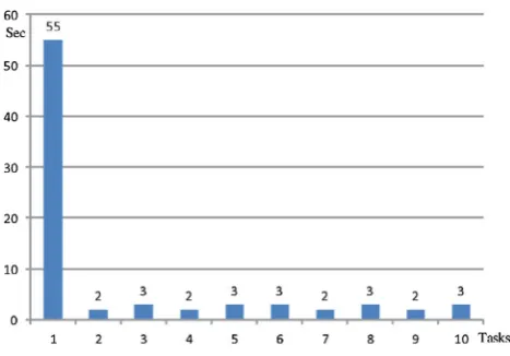
MapReduce is a popular programming model for Cloud computing and big data computing [25–27]. It exposes a simple programming API in terms of map and reduce func-tions. The simplicity of MapReduce is attractive for users, but the framework has several limitations. Applications such as machine learning and graph analytics iteratively process the data, which means multiple rounds of computation are performed on the same data. In MapReduce, every job reads its input data, processes it, and then writes it back to Hadoop Distributed File System (HDFS). For the next job to con-sume the output of a previously run job, it has to repeat the read, process, and write cycle. For iterative algorithms, which want to read once, and iterate over the data many times, the MapReduce model poses a significant overhead. As a typi-cal iterative algorithm, genetic algorithm needs many times iterative computations for evaluation of fitness function. To overcome the above limitations of MapReduce, Spark uses resilient distributed datasets (RDDs) which implement in-memory data structures and cache intermediate data across a set of nodes [28]. Since RDDs can be kept in memory, algo-rithms can iterate over RDD data many times very efficiently. In the paper, we make a simple experiment by evaluating the fitness function as a computing task. In Figs.3 and4, the horizontal axis is the number of tasks, and the vertical axis is the execution time. We can see that each Mapreduce task takes about 120 s, with 50 s for map and reduce operations and 70 s for shuffle and I/O jobs. In comparison, each Spark task takes only 3 s except for the first task, due to the first load data.
Fig. 3 Execution time of each task using MapReduce model
Fig. 4 Execution time of each task using Spark model
3 System model and problem formulation
3.1 System model
WDS, which consists of thousands of pipes, junctions and hydro-valves, may have a loop or branch network topology, or a combination of both. It is often modeled as a graph G=(V,E), where vertices inV represent junctions, tanks, or other sources, and edges inErepresent pipes, pumps, and valves. Drinking water flows are driven by pumping rates and pressure, which may vary frequently.
A contaminant eventa refers to the injection of poison substance by malicious attacks and may occur at any node, any time with uncertain dose of toxic chemicals or biological substance. The set of all possible contaminant scenarios A is infinite because of uncertainty, a representative set of sce-narios and quantify damages can be listed by enumeration or produced by random sampling.
assumed water demand. Most researchers rely on EPANET, a computer program developed by EPAs Water Supply and Water Resources Division as the main simulation tool [29].
For the convenience of analyzing sensor placement prob-lem, We make the following assumptions.
– A contamination event occurs at a single point in the network.
– The contaminant is conservative, i. e., it does not react with the substance in the water.
– Sensors are fixed at the junctions and protect downstream populations. A population is considered exposed if it could be reached by a flow path from the contamination point without passing a sensor.
– Water quality sensors work with two-value measurement, which means only a discrete yes/no indication of contam-ination is available from these sensors.
– Sensors are perfect, which mean they can detect con-taminants of any concentration with no false negatives and false positives; or they are capable to instantaneously detect a contaminant as soon as its concentration exceeds a minimum accepted value.
– A contamination warning is raised once a sensor detects a contamination event, and then response reactions are taken to isolate and flush contaminated water without any delay.
3.2 Problem formulation
Generally speaking, the objective of sensor placement in WDS is to detect contamination events and thus to mitigate the impact of contamination events. A typical mixed-integer programming (MIP) formulation for expected-impact sensor placement design is as follows.
min
a∈A αa
i∈La
daixai (1)
Constraint of equalities and inequalities are as follows:
i∈La
xai =1 ∀a∈ A (2)
xai ≤si ∀a ∈ A,i ∈La (3)
i∈L
cisi ≤ p (4)
si ∈ {0,1} ∀i ∈ L (5)
0≤xai ≤1 ∀a ∈ A,i ∈La (6)
This MIP minimizes the expected impact of a set of con-tamination incidents defined byA. For each incidenta∈ A,
αais the weight of incidenta, which is a probability of con-taminant injection.dai is the impact by contaminant eventa at nodei,L is a set of locations from the full set, where a location refers to a network node. For each incidenta,Lais the set of locations that can be contaminated by an incident a.
xaiis the decision variable, which indicates whether inci-dentais witnessed by a sensor at locationi. It is defined as continuous variables between 0 and 1. In practice, there is always an optimal solution wherexai is binary.
si is a binary decision variable, si = 1 indicates that a sensor are deployed atinode. Collectively, all of thesi vari-ables indicate where sensors are placed in the network; ci is the cost of placing a sensor at location i, and p is the budget. If the sensors are isomorphic, then pis a fixed num-ber.
The constraints of Eq. (2) assures that one sensor will send alerts for each incident. The constraints of inequal-ities (3) forbids a location from sending alerts if there is no sensor installed there. The third set of constraints enforces the limited budget for the total number of sen-sors.
Ostfeld et al. [8] defined four quantitative design objec-tives as contamination impact such as average detection time, average population affected prior to detection, aver-age consumption of contaminated water prior to detection, and average detection likelihood. These different objectives functions can be described by the impactdai. In the paper, we use average detection time as the performance criterion. That is, the lesser the average detection time is, the quicker we can detect the contaminant. Minimum average detection time can be defined as Eq. (7):
minαa
a∈A
Ti∈La(xai) (7)
where,Ti∈La(xai)is the minimum detection time when the incident a occurs and L nodes are deployed with sensors. Ideally, if the number of sensors is enough to deploy at each node in WSN, then they will give the earliest alarm to the full population as soon as the contaminants are injected into the WSN.
4 Algorithm design
4.1 Optimization framework
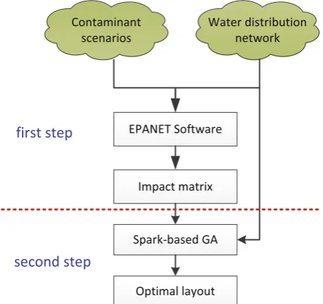
Fig. 5 Framework of optimization for SPP
first step is to simulate contamination incidents and compute contamination impact by the simulator EPANET [29], which is used to perform simulation of the hydraulic and water quality behavior within pressurized pipe network. Generally speaking, this process is time-consuming because contami-nation incidents are simulated for all network junctions, one for each hour of the day. After the simulation, the results of risk are stored in an impact matrix, and then the optimiza-tion algorithm can search the optimal placement of sensors according to the impact matrix. The framework of our method is shown in Fig.5.
From Fig.5, we can see that optimization process for SPP can be divided into two steps. The first step is to generate the contaminant events and use simulator (EPANET) to compute the impact matrix. And the second step is using optimization algorithm to select an optimal placement of sensors from the potential solution set.
4.2 Spark-based genetic algorithm
Genetic algorithm is inherently parallel since its fitness eval-uation and evolution process can be carried out concurrently. There are four parallel models for distribution algorithm: global model, distributed model, cellular model, and hybrid model [30].
As a master-slave distributed computing, Spark is suitable for the parallelization of the global and distributed model of genetic algorithm. Therefore, aiming to improve the perfor-mance and effectiveness of genetic algorithm, we use Spark to parallelize it. The proposed parallel genetic algorithm is based on Spark resilient distributed datasets. The whole
pop-ulation is stored as RDD and is cached in memory, which accelerates the subsequent processing.
We roughly divide our proposed algorithm into two phases. In the first phase, we initialize population, paral-lelize it into different partitions of RDD, and then evaluate fitness function of each individual on different workers. In the second phase, we perform the genetic operation on each indi-vidual after the parallel fitness evaluation value is returned to the driver. Then, we check whether the stop condition is satisfied. If it’s not met, the algorithm continues the fitness evaluation in Phase 1.
Algorithm 1 details the pseudo-code of our proposed approach. The required inputs include the impact matrix, the maximum generation, the size of population, the crossover rate and the mutation rate. The output is an optimal or near-optimal solution, which is the best placement of sen-sors.
As seen in Algorithm 1, the population is first initial-ized with popsize individuals, each individual is made up of s sensors that are deployed in WSN, then they are cached into different partitions of populationRDD (line 1–4). Subsequently, SGA performs the evaluation of the fitness function in parallel (line 6–8), the population with fitness value are counted by the driver. Next, SGA enters the second phase and executes evolution operations, such as crossover and mutation. And then a roulette selection operation is carried out according to the fitness value of each individual (line 9–14). Finally, if the results meet the stop condition, we output the best individual. Other-wise, SGA returns to the fitness evaluation phase (line 5).
As the evaluation of fitness function is the most time-consumed part, we implement the parallel algorithm on the Spark cluster. Algorithm2describes the pseudo-code of the process of fitness function evaluation.
Algorithm 1Spark-based Genetic algorithm Require:matrix. txt, maxgeneration,popsize, pc,pm
Ensure:optimal placement of sensors. 1:matrixRDD←parallelize(“matrix. txt”) 2:matrixRDD.persist();
3:population←initializePop(popsize);
4:populationRDD←Parallelize(population);
5:whilet< maxgenerationdo
6: foreach Individual Ij∈populationRDDdo
7: fitnessRDD←Ij.map(−.assessFitness())
8: end for
9: result←fitnessRDD.collect()
10: population(t)←sortByValue(result)
11: Selection:Ps(t)←select[population(t)]
12: Crossover:Pc(t)←crossover[(Ps(t),pc]
13: Mutation:Pm(t)←mutate[Pc(t),pm]
14: population(t+1)←Pm(t)
Algorithm 2Fitness Evaluation Require:matrixRDD,population
Ensure:population with fitness value
1:populationRDD←parallelize(“population”) 2:foreach Individual Ij∈populationRDDdo
3: foreach row∈matrixRDDdo
4: ftemp(t)←min(detection time)
5: ifftemp(t) >maxTimethen
6: ftemp(t)=0
7: rowNum←(rowNum−1)
8: else
9: f(t)=f(t)+ftemp(t)
10: end if
11: end for
12: fitnessRDD←f(t)÷rownNum
13:end for
14:fitness←fitnessRDD.collect()
15:return population with fitness value
In Algorithm2, the required inputs include the population and matrixRDD and the output is the population with fitness value. For the contaminant impact matrix, we first sort each rows and get the minimal detection time. Second, we sum up the minimal detection time for each rows and return the mean value as the fitness value (line 2–13). As the matrix has more than 25,000 rows and 10,000 columns, this part has the most significant computation overhead for our proposed SGA.
5 Experiment results and analysis
5.1 Experiment settings
In the experiment, we deploy 5 or 20 sensors in a large scale WSN as shown in Fig.2. In order to evaluate the placement of sensors, we first simulate the contamination scenarios. Each contaminant intrusions occur at random time with an injection flow rate of 125 L/h, contamination concentration of 230,000 mg/L, and injection duration of 2 h. The contaminant was assumed conservative after injection. Each contamina-tion scenario involved a single injeccontamina-tion locacontamina-tion, which may occur at any network node and begin at any time with equal probability. For purposes of design evaluation, contaminant concentrations were evaluated using a 5-min time step. A ran-domized impact matrix of 25,054 events (two injections at each node of the system, at two random times) was generated. To verify the performance of SGA, we implemented SGA on a cluster with eight servers. Each server is equipped with a 2.0 GHZ dual-core processor and 16 GB memory, as sum-marized in Table1.
The default parameters of SGA are listed in Table2.
5.2 Accuracy evaluation
To test and evaluate the accuracy of SGA, we performed two categories of experiments with 5 and 20 sensors in water
dis-Table 1 Cluster configuration
Number of servers 8
Processor 2.0 GHZ
Memory 16 GB
Operation System Ubuntu 12.04
Hadoop Hadoop-2.4.0
Spark Spark-1.4.0
Table 2 Spark-based Genetic
Algorithm Settings Crossover probability 0.95 Mutation probability 0.1 Elite strategy 10 Population size 80 Evolution generation 50
Fig. 6 Fitness value versus evolution generation, 5 sensors or 20 sen-sors are deployed in large scale WSN)
tribution network. Then we compared the performance with two other algorithms, i. e., the traditional genetic algorithm and the greedy algorithm [8].
Figure6shows that fitness function value decreases as the evolution generation increases from 1 to 50. The reason is that all of the three algorithms are convergent. In addition, it can be seen that the more sensors will lead to the reduction of average detection time. It should note that if we equip each node with one sensor, the average detection time is zero.
Table 3 Solution for 5 sensors
in a large WSN Algorithm Sensor location Average detection time Genetic algorithm 321, 3770, 4084, 4939, 7762 795
Greedy algorithm 10874, 4684, 11304, 3357, 11184 789 SGA 5240, 5665, 5883, 6107, 8897 257
Table 4 Solution for 20 sensors in a large WSN
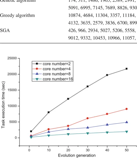
Algorithm Sensor location Average detection time Genetic algorithm 174, 311, 1486, 1905, 2589, 2991, 3548, 3757, 3864, 4184, 4238
5091, 6995, 7145, 7689, 8826, 9308, 9787, 10614, 12086 645 Greedy algorithm 10874, 4684, 11304, 3357, 11184, 1478, 9142, 1904, 4032, 9364, 4240
4132, 3635, 2579, 3836, 6700, 8999, 3747, 8834, 3229 665 SGA 426, 966, 2934, 5027, 5206, 5558, 5858, 6034, 6117, 6710, 7010, 7256
9012, 9332, 10453, 10966, 11057, 11126, 11431, 11753 130
Fig. 7 Task execution time versus the number of evolution generation, 20 sensors are deployed in water distribution networks)
5.3 Efficiency evaluation
After showing the accuracy of our SGA, we further evaluate its efficiency in the metric of task execution time as well as the derived fitness value.
We first varied the generation number under cluster size (i. e., the number of CPU cores) 2, 4, 8 and 16 to check how it affects the task execution time in the metric of seconds. Figure7shows the task execution time under different gen-eration numbers ranging from 1 to 50. It can be first seen that the task execution time is proportional to the generation number in SGA. This is simply because larger generation numbers require longer evolution time, which further incurs longer task execution time. On the other hand, we can also see that larger cluster size also indicates shorter task exe-cution time. This implies that SGA efficiently explores the available cloud resources.
Fig. 8 Average detection time versus evolution generation, 20 sensors are deployed in large scale water distribution networks)
Next, we investigated how the generation number affects the optimization objective, i.e., average detection time. The results are shown in Fig.8. On the contrary, we can see that increasing the generation number is beneficial to the fitness value. However, the benefit becomes marginal when the gen-eration number is large enough. The nature of the evolution computation determines that the quality of the generation may finally converge. Although average detection time of four cases reduces with the increment of the number of gen-erations, their rates of convergence are different because of the randomness of genetic algorithm.
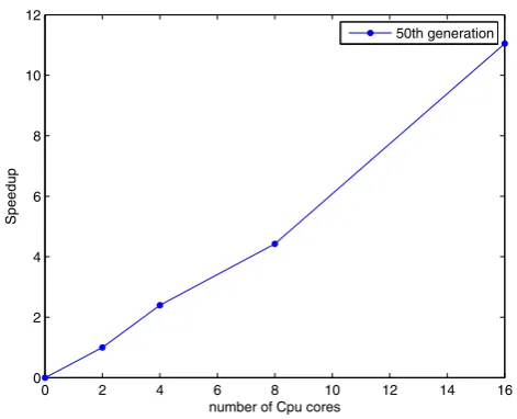
Finally, we check how the cluster size influences the task execution time in the metric of speedup ratioSpeedup, we defineSpeedupas the formula (8).
0 2 4 6 8 10 12 14 16 0
2 4 6 8 10 12
number of Cpu cores
Speedup
50th generation
Fig. 9 Speedup versus the number of CPU cores
In formula (8),T1is the task execution time of one server with
two CPU cores, andTpis the task execution time of cluster withpCPU cores. Figure9presents evaluation results with the number of CPU cores ranging from 2 to 16. We note that the speedup scales well with the cluster size.
6 Conclusion
In this paper, we proposed a Spark-based genetic algorithm for sensor placement in water distribution system. Based on the global and distributed model of GA Parallelization, SGA is divided into two phases. The first phase is the fitness evalua-tion that calculates each individual’s fitness value on workers. The second phase is the genetic operations which run on the driver node. We evaluated the performance of SGA in terms of accuracy, efficiency and speedup. Results show that SGA outperforms the other two algorithms in the term of accuracy. We also find that SGA has a nearly linear speed-up for the parallel processing of sensor placement problem.
We have also identified a number of issues to be investi-gated in future studies with the following being noteworthy:
1. Investigation of the robustness of the proposed algorithm by applying it to a larger scale drinking water distribution networks and test it on a large size cluster.
2. Incorporation of the ability of sensors and accuracy of the hydraulic model into the proposed algorithm for realistic applications.
Acknowledgements This research was supported in part by the NSF of China (Grant No. 61305087, 61673354, 61672474, 61501412). Ming Li’s research is partially supported by US National Science Founda-tion Award (Grant No. 1626586). This paper has been subjected to Hubei Key Laboratory of Intelligent Geo-Information Processing within School of Computer Science, China University of Geosciences, Wuhan,
China, 430074. It was also supported by Open Research Project of The Hubei Key Laboratory of Intelligent Geo-Information Processing (KLIGIP201603, KLIGIP201607).
References
1. Hrudey, S., Payment, P., Huck, P., Gillham, R., Hrudey, E.: A fatal waterborne disease epidemic in Walkerton, Ontario: comparison with other waterborne outbreaks in the developed world. Water Sci. Technol.47(3), 7–14 (2003)
2. Kou, J.: Drinking water reservoirs were poisoned in Ruyang City of Henan Province. http://news.china.com/zh_cn/social/ 1007/20031004/11549967.html
3. Hart, W.E., Berry, J.W., Boman, E.G., Phillips, C.A., Riesen, L.A., Watson, J.: Limited-memory techniques for sensor placement in water distribution networks. In: Learning and Intelligent Optimiza-tion. Springer, Berlin (2008)
4. Zeng, D., Gu, L., Lian, L., Guo, S., Yao, H., Hu, J.: On cost-efficient sensor placement for contaminant detection in water distribution systems. IEEE Trans. Ind. Inf.11, 112–121 (2016)
5. Xu, J., Johnson, M.P., Fischbeck, P.S., Small, M.J., Vanbriesen, J.M.: Robust placement of sensors in dynamic water distribution systems. Eur. J. Oper. Res.202(3), 707–716 (2010)
6. Bergerwolf, T.Y., Hart, W., Saia, J.: Discrete sensor placement problems in distribution networks. Math. Comput. Model.42(13), 1385–1396 (2005)
7. Carr, R.D., Greenberg, H.J., Hart, W.E., Konjevod, G., Lauer, E., Lin, H., Morrison, T., Phillips, C.A.: Robust optimization of con-taminant sensor placement for community water systems. Math. Program.107(1–2), 337–356 (2006)
8. Ostfeld, A., Uber, J.G., Salomons, E., Berry, J.W., Hart, W.E., Phillips, C.A., Watson, J.-P., Dorini, G., Jonkergouw, P., Kapelan, Z., et al.: The battle of the water sensor networks (BWSN): a design challenge for engineers and algorithms. J. Water Resour. Plan. Manag.134(6), 556–568 (2008)
9. Krause, A., Leskovec, J., Guestrin, C., VanBriesen, J., Faloutsos, C.: Efficient sensor placement optimization for securing large water distribution networks. J. Water Resour. Plan. Manag.134(6), 516– 526 (2008)
10. Chang, N.-B., Prapinpongsanone, N., Ernest, A.: Optimal sen-sor deployment in a large-scale complex drinking water network: comparisons between a rule-based decision support system and optimization models. Comput. Chem. Eng.43, 191–199 (2012) 11. Gong, W., Cai, Z.: Differential evolution with ranking-based
muta-tion operators. IEEE Trans. Syst. Man Cybernet.43(6), 2066–2081 (2013)
12. Yang, M., Li, C., Cai, Z., Guan, J.: Differential evolution with auto-enhanced population diversity. IEEE Trans. Syst. Man Cybernet.
45(2), 302–315 (2015)
13. Von Laszewski, G., Wang, L., Wang, F., Fox, G.C., Mahinthakumar, G.K.: Threat detection in an urban water distribution systems with simulations conducted in grids and clouds. In: Proceedings of the Second International Conference on Parallel, Distributed, Grid and Cloud Computing for Engineering, Ajaccio, Corsica, France (2011) 14. Wu, Z., Khaliefa, M.: Cloud computing for high performance opti-mization of water distribution systems. In: Proceedings of Albu-querque, New Mexico, World Environmental and Water Resources Congress (2012)
15. Shen, H., McBean, E.A.: Application of parallel computing in data mining for contaminant source identification in water distribution systems. Can. Water Resour. J.38(1), 34–39 (2013)
17. Rathi, S., Gupta, R.: A critical review of sensor location methods for contamination detection in water distribution networks. Water Qual. Res. J. Can.50(2), 95–108 (2015)
18. Wu, J., Zhu, X., Zhang, C., Yu, P.S.: Bag constrained structure pattern mining for multi-graph classification. IEEE Trans. Knowl. Data Eng.26(10), 2382–2396 (2014)
19. Wu, J., Pan, S., Zhu, X., Zhang, P., Zhang, C.: SODE: self-adaptive one-dependence estimators for classification. Pattern Recogn.51, 358–377 (2016)
20. Guan, J., Aral, M.M., Maslia, M.L., Grayman, W.M.: Optimization model and algorithms for design of water sensor placement in water distribution systems. In: 8th Annual Symposium on Water Dis-tribution Systems Analysis. Environmental and Water Resources Institute of ASCE (EWRI of ASCE) New York, pp. 1–16 (2006) 21. Liu, S., Auckenthaler, P.: Optimal sensor placement for event
detec-tion and source identificadetec-tion in water distribudetec-tion networks. J. Water Supply63(1), 51–57 (2014)
22. Schwartz, R., Lahav, O., Ostfeld, A.: Optimal sensor placement in water distribution systems for injection of chlorpyrifos. In: World Environmental and Water Resources Congress 2014@ sWa-ter Without Borders. ASCE, pp 485–494 (2014)
23. Afshar, A., Mariño, M.A.: Multi-objective coverage-based aco model for quality monitoring in large water networks. Water Resour. Manag.26(8), 2159–2176 (2012)
24. Ma, Y., Wang, L., Liu, D., Liu, P., Wang, J., Tao, J.: Generic par-allel programming for massive remote sensing data processing. In: International Conference on Cluster Computing, pp 420–428 (2012)
25. Dean, J., Ghemawat, S.: MapReduce: simplified data processing on large clusters. In: Operating Systems Design and Implementation, vol. 51(1), pp 107–113. Prentice-Hall, Upper Saddle River (2008) 26. Wang, L., Tao, J., Ranjan, R., Marten, H., Streit, A., Chen, J., Chen, D.: G-Hadoop: Mapreduce across distributed data centers for data-intensive computing. Future Gen. Comput. Syst.29(3), 739–750 (2013)
27. Zhao, J., Wang, L., Tao, J., Chen, J., Sun, W., Ranjan, R., Kolodziej, J., Streit, A., Georgakopoulos, D.: A security framework in G-Hadoop for big data computing across distributed cloud data centres. J. Comput. Syst. Sci.80(5), 994–1007 (2014)
28. Zaharia, M., Chowdhury, M., Das, T., Dave, A., Ma, J., Mccauley, M., Franklin, M.J., Shenker, S., Stoica, I.: Resilient distributed datasets: a fault-tolerant abstraction for in-memory cluster com-puting. Technical Report (2012)
29. U.S. EPA: Tutorial threat ensemble vulnerability analysis—sensor placement optimization tool TEVA-SPOT graphical user interface, version 2.2.0 Beta, EPA-600-R-08-147. Office of Research and Development, National Homeland Security Research Center, vol. 1(1), pp. 1–183 (2009)
30. Luque, G., Alba, E.: Parallel Genetic Algorithms: Theory and Real World Applications, vol. 367. Springer, Berlin (2011)