Article
A Comparison of Streamflow and Baseflow Responses
to Land-Use and Climate Change Using SWAT
Mohamed Aboelnour 1,2, Margaret W. Gitau 1 and Bernard Engel 1,*
1 Department of Agricultural & Biological Engineering, Purdue University, West Lafayette, IN, 47906; USA; [email protected]; [email protected]
2 Geology Department, Faculty of Science, Suez Canal University, Ismailia, 41511, Egypt * Correspondence: [email protected];
Abstract: Alteration of land use and climate change are among the main variables affecting watershed hydrology. Characterizing the impacts of climate variation and land use alteration on water resources is essential in managing watersheds. Thus, in this research, streamflow and baseflow responses to climate and land use variation were modeled in two watersheds, the Upper West Branch DuPage River (UWBDR) watershed in Illinois and Walzem Creek watershed in Texas. The variations in streamflow and baseflow were evaluated using the Soil and Water Assessment Tool (SWAT) hydrological model. The alteration in land use between 1992 and 2011 was evaluated using transition matrix analysis. The non-parametric Mann-Kendall test was adopted to investigate changes in meteorological data from 1980-2017. Our results indicated that the baseflow accounted for almost 55.3% and 33.3% of the annual streamflow in the UWBDR and Walzem Creek watersheds, respectively. The contribution of both land use alteration and climate variability on the flow variation is higher in the UWBDR watershed. In Walzem Creek, the alteration in streamflow and baseflow appears to be driven by the effect of urbanization more than that of climate variability. The results reported herein are compared with results reported in recent work by the authors in order to provide necessary information for water resources management planning, as well as soil and water conservation, and to broaden the current understanding of hydrological components variation in different climate regions.
Keywords: Streamflow, baseflow, SWAT, urbanization, climate alteration, Mann-Kendall.
1. Introduction
Ecosystems and humans are fundamentally dependent on different water resources. Thus, for the general development of any country, the quality and the quantity of these water resources flowing through rivers is of vital importance to socio-economic development [1]. Issues related to changes in water resources are commonly evaluated around the globe [2,3,4]. In the United States, evaluation of streamflow and baseflow have been documented [5,6,7]. However, the quantitative change in streamflow and baseflow has yet to be evaluated across different climatic conditions.
Climate alterations and human actions both act as stressors to place severe pressure on water resources [8,9]. The variations in climate and land use directly impact total streamflow, interflow, surface runoff and baseflow, causing events of droughts and floods that impact the sustainability of these resources and the social ecosystem [10]. Several studies have examined alterations in streamflow due to changes in temperature and precipitation [11,12,13], urbanization [14] and land use change [2,15]. Baseflow is the portion of streamflow sustained in a river by delayed pathways. Baseflow is often assumed to be equal to groundwater recharge [16]. It provides a relatively high water quality with a high clarity and stable temperature, and is considered indicative of sustained streamflow during dry periods of the season, which is important to stream biota and helps recreation based industries [17]. This low-flow data is essential in understanding the current and future changes
to watershed hydrology. Several reports have indicated that the change in baseflow over time is due to variations in agricultural management [18], climate change [8], urbanization [19], and land use alteration [20]. Therefore, in order to develop scenarios for water resources evaluation, land use change and climate variation are usually chosen as the main influencing factors. The impacts of climate variation and urbanization on streamflow and baseflow are reviewed in Aboelnour et al. [8] and Price [21].
Different methods have been used to evaluate the response of watershed streamflow and baseflow to human activities and climate change. These techniques include hydrologic similarities within the watersheds, paired catchments, statistical methods and hydrological modeling [22]. Since climate and land use change need to be investigated on a local scale and can vary from place to place [23], there is a need to use comprehensive and physical tools to evaluate as much information as possible from the limited existing data [24]. Hence, hydrological models are considered the most appealing approach to carry out impact assessment studies. They provide a conceptualized framework and are suitable for use as part of scenario studies on the relationship between hydrological components, climate variability, and land use change [25,26]. Among these models is the Soil and Water Assessment Tool (SWAT) model.
The SWAT model, developed by the United States Department of Agricultural (USDA) Agriculture Research Service, is designed to model hydrology at the scale of a watershed [27]. SWAT is widely used around the world to evaluate the influences of ecological and environmental alterations and for hydrological processes at different catchment scales, even with a limited amount of data [10,28]. In addition, it offers several software tools, and was therefore selected for this research. Each watershed was divided into smaller sub-basins in the SWAT model. These sub-basins were then divided into smaller HRUs that were fundamentally based on land use, soil type and slope [29]. Within each HRU, the Soil Conservation Service (SCS) curve number and Green-Ampt infiltration are adapted to compute surface runoff using daily precipitation. In addition, SWAT subdivides the groundwater system into deep confined aquifers that contribute to flow outside of the catchment, and shallow unconfined ones, in which the groundwater and baseflow return back to the stream [30]. The SWAT model has proven to perform well in streamflow and baseflow simulations around the world and in complex catchments with extreme events [31], since it allows the interconnections of different physical processes [32,33,34]. Therefore, in this research, the SWAT model was adopted to assess the impacts of land use and climate change.
Streamflow and baseflow responses to human activities, urbanization and climate variation are different in various basins with respect to climate regions, geographical variances, scale and urbanization levels [21,35]. However, the need to fully understand the streamflow and baseflow responses to external stimuli is of vital importance. Many studies in the last few years have been carried out to investigate the hydrological response to urbanization and climate change [36,13]. Outputs of these studies can help in understanding the cause of shifts in water resources. However, these studies mainly focus on the single impact of either land use change or climate variation, but neglect the combined effects of climate alteration and human activities and their contributions to the change. Thus, the combined effects are still not fully understood over different climatic conditions and geographical regions. For this reason, the responses of streamflow and baseflow to urbanization and climate variation will be evaluated for varying climate conditions with different urbanization levels. Two watersheds, the Upper West Branch DuPage River (UWBDR) watershed, Illinois, and Walzem Creek watershed, Taxes, will be used as examples to quantify the changes in streamflow and baseflow as a response to climate and land use change.
watersheds in Cook County, northeastern Illinois. They found that urbanization had a greater impact than climate on the increase in flood discharge, and due to increasing urbanization, discharge volume may become even higher in the future. In addition to floodplain management, wetland protection, bank stabilization, stream restoration, water quality, and groundwater recharge are also concerns within the catchments. Some sections of the stream are supplied with a substantial amount of their baseflow from local groundwater discharge, while other sections release baseflow to groundwater due to the presence of a large outwash plain at the base of West Chicago Moraine that creates conditions that promote rapid flooding and groundwater movement from the border of the moraine through the outwash [37].
The second watershed is the Walzem Creek, San Antonio, Texas. The city of San Antonio, Bexar County and other partners initiated a watershed protection plan in 2006 for the Upper San Antonio basin, including the Walzem Creek watershed, to track efforts that enhance urban outreach, and to bring the basin back into compliance with water resource and water quality recreation standards. In 2015, the Environmental Protection Agency (EPA) approved this protection plan, making the state eligible for project funding within the watershed to address nonpoint source runoff. The report can be viewed at https://www.brwm-tx.org/. A combination of rocky and clay soils contribute to larger runoff than groundwater flow in this watershed. Rock, clay, and slopes create nearly impervious conditions in the northern portion of the watershed and thus reduce the effect of development and its associated impervious cover on storm water flow [39].
The main target of this study is to evaluate the impact of separate and combined impacts of land use changes and climate alteration on streamflow and baseflow in two watersheds under different land use and climatic conditions. The specific goals of this research are: (1) identify the long term trend and the abrupt changes in hydrological and meteorological data; (2) determine the change in land use maps from 1992 to 2011; (3) use the new calibrated and validated SWAT model to assess the individual and combined impacts of land use change and climate variation on streamflow and baseflow; and (4) compare the outputs of this study with the findings of Aboelnour et al. [8]. Information gleaned from this study can be used to understand the variations in hydrological flow components, and are necessary for water resources management and planning, as well as water and soil conservation in geographically different watersheds.
2. Study areas
2.1 Upper West Branch DuPage River watershed
The Upper West Branch DuPage River watershed (UWBDR) is located in northeast Illinois, within the six-county Chicago metropolitan region. The watershed is located approximately in the western one third of DuPage County (Figure 1). The headwaters originate in the northwestern part of Cook County where the water flows generally to the south into and through DuPage County. The UWBDR is part of the West Branch DuPage River (WBDR) watershed that divides into upper, middle and lower branches within the DuPage catchment and belongs to the Des Plaines River basin. The UWBDR covers approximately 91.7 km2 (USGS Gauge 05539900) with mean annual precipitation
ranging from 612 to 1293 mm from 1980 to 2017, and average annual temperatures ranging from 8.4 to 12.5 °C. The minimum, maximum and mean elevations in the area are 217, 298 and 240 meters above sea level, respectively. Land use varies from residential (77.2%) to forest (4%), vacant (4.1%), and cultivated (2.4%). The river network in the watershed receives treated effluent and wastewater from the cities of West Chicago, Illinois [40].
2.2 Walzem Creek
Gauge 08178800), with a mean annual precipitation ranging from 320 to 1200 mm and average annual temperatures ranging 19.3 to 22.3 °C. Mean elevation in the area is 204 meters, with a minimum and maximum of 152 and 266 meters above sea level, respectively. Similar to the UWBDR watershed, most of Walzem Creek is covered with developed areas (92.5%); however, other land uses varies from wetlands (7.8%), shrublands (4.5%) and forests (2.8%). This area is a large portion of the Upper San Antonio Watershed, hence, it contributes a large amount of total streamflow. According to the main Koppen-Geiger climate classes for US counties, the San Antonio, Bexar County area lies at the border between warm, humid, equatorial zone and fully hot arid and steppe zone [41]. Therefore, this watershed will be representative of semi-arid regions.
Figure 1: Index map showing location of the study watersheds: Upper West Branch DuPage River in Illinois (right) and Walzem Creek in Texas (left)
3. Materials and Methods
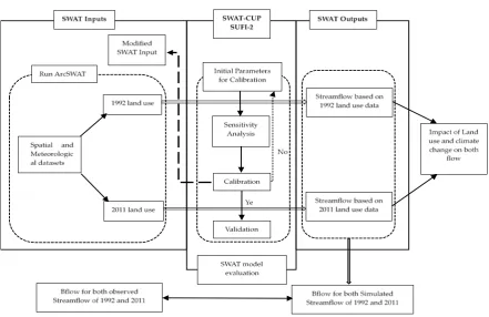
The data described herein includes spatial topography, Digital Elevation Model (DEM), land use and soil data, and hydro-meteorological data. Data analysis procedures and methods used are detailed extensively in Aboelnour et al. [8]. A flow chart depicting procedures used in this study is summarized in Figure. 2.
3.1 Data development
3.1.1 Spatial data
Two raster land use maps for the years 1992 and 2011 were obtained from the National Map Viewer (NMV). Digital Elevation Model (DEM) data were acquired from the Geospatial Data Gateway (GDG) with a resolution of 10 m. Soil Survey Geographic Data (SSURGO) data were used in this research with a resolution ranging from 1:12,000 to 1:63,630. Land use, soil type and slope were then used to divide the delineated sub-basins into a small series of uniform Hydrologic Response Units (HRUs) that represent the smallest representative units within the watershed [42].
3.1.2 Hydro-meteorological data
(NCDC). The meteorological weather stations were 12 kilometers and 0.8 kilometer away from the borders of the UWBDR and Walzem Creek watersheds, respectively.
3.2 Mehodology
3.2.1 Baseflow separation
Baseflow measurements were separated from daily streamflow data acquired from USGS gauged stations using the automatic baseflow digital filter method (Bflow). The Bflow filter separates streamflow data into baseflow and surface runoff by passing the observed streamflow through the filtering equation three times [43,44]:
𝐵𝐵𝐵𝐵𝑡𝑡=𝛼𝛼×𝐵𝐵𝐵𝐵𝑡𝑡−1+1− 𝛼𝛼2 × (𝑄𝑄𝑡𝑡+𝑄𝑄𝑡𝑡−1) (1)
where 𝐵𝐵𝐵𝐵 is the baseflow, 𝛼𝛼 is the filter parameter (0.925), 𝑄𝑄 is the total streamflow, and t is the time step. Equation 1 is applied only when BF ≤ Qt [45].
3.2.2 Soil and Water Assessment Tool (SWAT) model calibration and validation
The monotonic trends in the historical meteorological data were evaluated using the modified Mann-Kendall (MK) test developed by Hamed and Rao [46]. Based on the abrupt change in the trends in precipitation and temperature using the MK test, the study period from 1980 to 2017 was split into two time spans, 1980 to1998 and 1999 to 2017, with a breakpoint in 1998. The period 1980-1998 was assigned as a baseline for model calibration and validation. The model simulation time was segmented into a warm up period (1980-1983), calibration period (1984-1993), and validation period (1994-1998). The SWAT model calibration and validation were performed using the land use map of 1992 and streamflow data from 1980 to 1998 for each of the selected watersheds. Model optimization, sensitivity analysis, calibration, validation and uncertainty analysis of parameters were carried out using the Sequential Uncertainty Fitting program algorithm (SUFI-2) approach within the SWAT-CUP interface developed by Abbaspour et al. [47]. Based on Aboelnour et al. [8], the twenty hydrologic parameters listed in Table 1 were used in this study for the UWBDR and Walzem Creek watersheds calibration of streamflow and baseflow. However, sensitivity analysis using the SUFI-2 global sensitivity analysis was carried out in the first stage due to the presence of a large number of parameters within the SWAT model [44]. Only parameters sensitive for the watersheds were then used in the calibration process and optimized based on monthly values [48]. Both automatic and manual calibration were carried out to allow qualitative and quantitative comparisons of the values, to fine tune the values of the auto-calibrated parameters, as well as to decrease the differences between the observed and simulated outputs [49].
3.2.3 Model sensitivity analysis
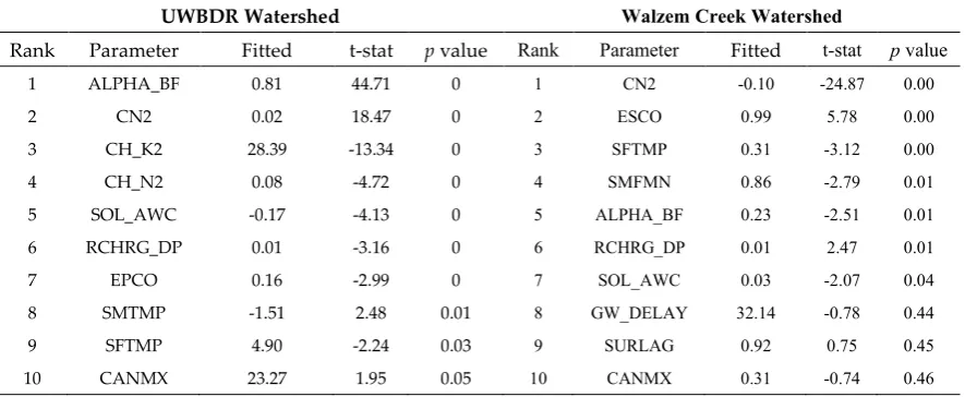
The global sensitivity analysis procedures showed that the sensitive parameters obtained from the LEC in Aboelnour et al. [8] were critical in the case of the UWBDR watershed, but with a different rank order. It was also found that these rankings were impacted by the selected objective function in the model. For example, curve number (CN2), soil evaporation compensation factor (ESCO), snowfall temperature (SFTMP), melt factor for snow (SMFMN), baseflow recession constant (ALPHA_BF), and deep aquifer percolation fraction (RCHRG_DP) were the most critical parameters in UWBDR when KGE was selected to be the objective function incorporated in the model (Table 2). These parameters characterize surface runoff, soil properties and groundwater.
indicated a rapid response to groundwater recharge. However, the lower baseflow recession constant in the UWBDR indicated large storage discharge and slow drainage in the shallow aquifer, which might be attributed to the complex geological structure of the watershed such as the presence of folds and faults [36]. The high deep aquifer percolation parameter (RCHRG_DP) in Walzem Creek indicated the increase of water movement to the deep aquifer. SOL_AWC represented the soil moisture content and hence played a role in surface runoff and was considered to be directly proportional to the soil’s ability to hold water, affecting streamflow.
Table 1. SWAT input parameters used for the UWBDR and Walzem Creek watersheds calibration of streamflow and baseflow [8]
Parameter 1Ext. Description Adjustment 1IV 1LB 1UB
Parameters controlling water balance
ESCO hru Soil evaporation compensation factor R 0.95 0.01 1
EPCO hru Plant uptake compensation factor R 1 0.01 1
CANMX hru Max canopy storage R 0 0 25
SFTMP bsn Snowfall temp R 1 -5 5
SMTMP bsn Snowmelt base temp R 0.5 -5 5
TIMP bsn Snow back temp lag factor R 1 0.01 1
SMFMX bsn Melt factor for snow on June 21 R 4.5 0.01 10
SMFMN bsn Melt factor for snow on Dec. 21 R 4.5 0.01 10
Parameters controlling surface water response
CN2 mgt Initial SCS Curve number V -- -0.25 0.25
SURLAG bsn Surface runoff lag coefficient R 4 0.1 10
Parameters controlling sub-surface water response
ALPHA_BF gw Baseflow alpha factor R 0.048 0.01 1
GWQMN gw Depth of water for return flow R 1000 0.01 5000
GW_DELAY gw Groundwater delay time R 31 0.1 50
REVAPMN gw Depth of water for evaporation R 750 0.01 250
GW_REVAP gw Groundwater evaporation coefficient R 0.02 0.02 0.2
RCHRG_DP gw Deep aquifer percolation fraction R 0.05 0.01 1
Parameters controlling soil’s physical properties
SOL_AWC sol Available water capacity of the soil water V -- -0.25 0.25
SOL_K sol Saturated hydraulic conductivity V -- -0.15 0.15
Parameters controlling channel’s physical properties
CH_K2 rte Effective hydraulic conductivity R 0 5 300
CH_N2 rte Main channel Manning’s “n” R 0.014 0.01 0.15
1Ext: Extension, R: Replace by value, V: Multiply by value, IV: Initial values, LB: Lower bound, UB: Upper bound
3.2.4 Statistical criteria and model evaluation performance
The performance of the SWAT model can be computed using statistical indices and graphical comparisons [52]. For the simulated streamflow and baseflow, the coefficient of determination (R2),
Nash–Sutcliffe model efficiency (ENS), PBIAS and modified Kling–Gupta Efficiency (KGE) were adopted to evaluate the model performance [53,54]. The monthly statistical streamflow and baseflow values for the calibrated models were adopted to evaluate the model performance. The performance of the SWAT model is considered good on a monthly basis when R2 > 0.75; ENS and KGE > 0.7; and
Table 2. Top 10 optimized SWAT sensitive parameter values in the UWBDR watershed and Walzem Creek watershed
UWBDR Watershed Walzem Creek Watershed
Rank Parameter Fitted t-stat p value Rank Parameter Fitted t-stat p value
1 ALPHA_BF 0.81 44.71 0 1 CN2 -0.10 -24.87 0.00
2 CN2 0.02 18.47 0 2 ESCO 0.99 5.78 0.00
3 CH_K2 28.39 -13.34 0 3 SFTMP 0.31 -3.12 0.00
4 CH_N2 0.08 -4.72 0 4 SMFMN 0.86 -2.79 0.01
5 SOL_AWC -0.17 -4.13 0 5 ALPHA_BF 0.23 -2.51 0.01
6 RCHRG_DP 0.01 -3.16 0 6 RCHRG_DP 0.01 2.47 0.01
7 EPCO 0.16 -2.99 0 7 SOL_AWC 0.03 -2.07 0.04
8 SMTMP -1.51 2.48 0.01 8 GW_DELAY 32.14 -0.78 0.44
9 SFTMP 4.90 -2.24 0.03 9 SURLAG 0.92 0.75 0.45
10 CANMX 23.27 1.95 0.05 10 CANMX 0.31 -0.74 0.46
3.2.5 Scenarios separating the impact of land use change and climate change
In this research, the “change-fix” approach used in Aboelnour et al. [8] was applied in order to evaluate the streamflow and baseflow as a response to separate and combined impacts of urbanization and climate alteration. Land use maps of 1992 and 2011 were used to represent the two time periods. The land use map of 1992 was adopted to represent the patterns in the first period (1980-1998), herein called TS1. On the other hand, the 2011 land use map was used to represent the second time span (1999-2017), herein called TS2.
A combination of four simulations were developed to evaluate the natural and human impacts on hydrology: (1) 1992 land use and TS1 climate data of 1980–1998 (X1); (2) 2011 land use and TS1 climate data of 1980–1998 (X2); (3) 1992 land use and TS2 climate data of 1999–2017 (X3); and (4) 2011 land use and TS2 climate data of 1999–2017 (X4). The well-calibrated SWAT model, using the land use data of 1992 and first climate period, was used to run the other four scenarios (X1 to X4). The simulated output values obtained from these scenarios were compared to the corresponding baseline model. X1 represents the baseline scenario with the corresponding circumstances, while the difference between X4 and X1 simulation describes the combined effects of land use change and climate variation. The comparison between X1 and X2 attempts to depict the separate impact of land use change. Finally, the differences between X3 and X1 outputs emphasize the individual impact of climate alteration.
3. Results and discussion
3.1. Trends in hydrologic components
Figure 2: Flow chart showing the methodology used in this study (modified from Aboelnour et al. [8])
Table 3. Temporal trends in annual streamflow and baseflow in the study areas
Streamflow Baseflow
UWBDR watershed
τ
-Stat 2.238 1.848Slope 3.195 1.301
α 0.001 > 0.1
Walzem Creek
τ
-Stat 0.277 -1.961Slope 2.043 -3.335
α > 0.1 0.001
The increase in average precipitation played an important role in the increasing trend of streamflow for the UWBDR watershed, while the slight increase in streamflow at Walzem Creek was accompanied by decreased precipitation. Moreover, human activity, such as construction of urban areas on agricultural areas, played a vital role in the amount of streamflow and baseflow.
(a) (b)
(c)
(d)
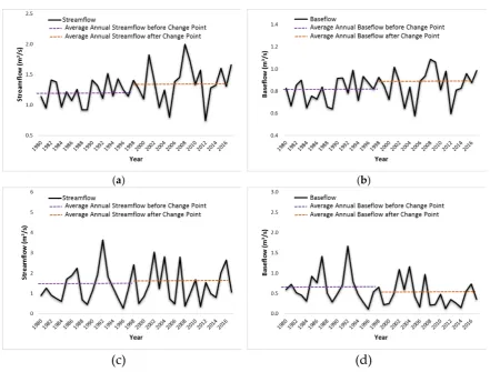
Figure 3. The MK trends for average daily streamflow (a) and baseflow (b) in the UWBDR watershed; average daily streamflow (c) and baseflow (d) in the Walzem Creek watershed
3.2. Trends in climatic components
The MK test was furthermore employed to quantify the monotonic trends of precipitation and temperature in the selected watersheds. Compared to the first climate period (1980-1998), statistical results indicated that the mean air temperature increased by 0.7 ᴼC (from 9.7 °C to 10.4 °C) and 0.6
ᴼC (from 20.7 °C to 21.3 °C) during TS2 at the UWBDR and Walzem Creek watersheds, respectively. Average annual precipitation increased by 9.1% (82 mm, from 890 mm to 972 mm) during TS2 in the UWBDR, while decreasing by 6.5% (56 mm, from 858 mm to 802 mm) in Walzem Creek (Figure 4).
(a) (b)
(c)
(d)
Figure 4. The MK trends forannual precipitation (a) and temperature (b) in the UWBDR watershed; and annual precipitation (c) and temperature (d) in the Walzem Creek watershed
Table 4. Temporal trends in annual precipitation and temperature in the study areas
Precipitation Temperature
UWBDR
τ
-Stat 0.503 2.709Slope 0.821 0.037
α > 0.1 0.001
Walzem
τ
-Stat 0.327 3.640Slope 1.179 0.036
Table 5. Summary of significance test and trend analysis for monthly precipitation and temperature in the UWBDR and Walzem Creek watersheds
UWBDR Walzem Creek
τ
-Stat Slope Sig p-valueτ
-Stat Slope Sig p -valueJan PRCP 1.245 0.551 NS 0.106 0.704 0.564 NS 0.240 TEMP 0.805 0.045 NS 0.210 1.722 0.051 NS 0.042
Feb PRCP 0.905 0.409 NS 0.183 -0.905 -0.142 NS 0.183 TEMP 0.339 0.005 NS 0.367 2.351 0.071 S 0.009
Mar PRCP 0.126 0.035 NS 0.450 0.855 0.248 NS 0.196 TEMP 0.729 0.043 NS 0.233 1.685 0.048 NS 0.046
Apr PRCP 0.805 0.425 NS 0.211 0.629 0.992 NS 0.265 TEMP 1.383 0.036 NS 0.083 1.722 0.038 NS 0.043
May PRCP 1.584 0.988 NS 0.057 -0.704 -0.268 NS 0.241 TEMP 0.981 0.024 NS 0.163 0.893 0.017 NS 0.186
Jun PRCP 1.534 1.364 NS 0.061 -1.282 -1.678 NS 0.100 TEMP 2.012 0.051 S 0.022 1.798 0.03 NS 0.036
Jul PRCP -0.427 0.581 NS 0.335 0.729 0.741 NS 0.233 TEMP 0.465 0.014 NS 0.321 1.031 0.013 NS 0.151
Aug PRCP -0.805 -1.349 NS 0.210 -0.641 0.493 NS 0.261 TEMP 1.358 0.021 NS 0.087 1.585 0.025 NS 0.056
Sep PRCP -0.855 -0.442 NS 0.196 1.383 1.52 NS 0.083 TEMP 2.364 0.054 S 0.009 1.245 0.019 NS 0.107
Oct PRCP 0.151 0.25 NS 0.440 -0.930 -0.547 NS 0.176 TEMP 2.087 0.058 S 0.018 1.207 0.031 NS 0.114
Nov PRCP -2.024 -1.669 S 0.021 -1.471 -0.504 NS 0.071 TEMP 1.320 0.043 NS 0.093 1.886 0.042 NS 0.030
Dec PRCP -0.226 -0.324 NS 0.411 0.176 -0.238 NS 0.430 TEMP 0.566 0.051 NS 0.286 1.119 0.04 NS 0.132
1 Significant level (α) = 0.05. S: Significant. NS: Not significant 3.3. Changes in land use characteristics
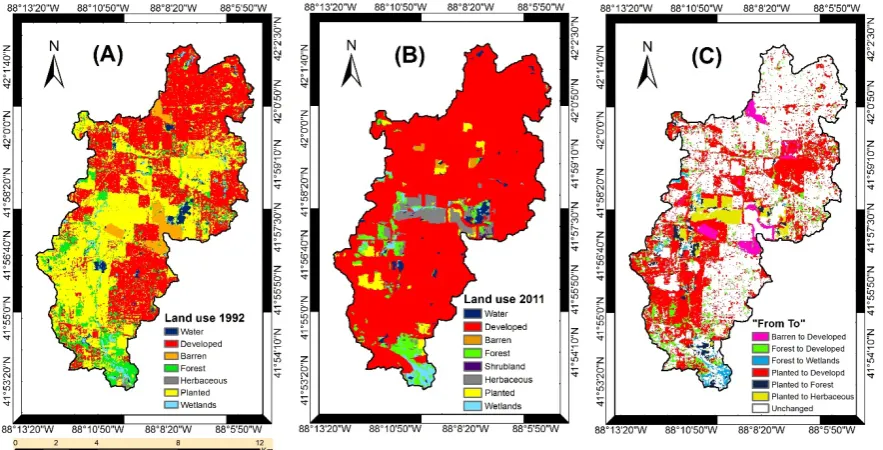
Cross tabulation analysis and post classification comparison were applied to evaluate the quantity of temporal conversions and nature of changes from one land cover category to another in land use maps of 1992 and 2011 [61,62]. In the UWBDR, a comparison of land use maps for the years 1992 and 2011 indicated that the most significant changes occurred in three classes: developed urban, planted and forest (Figure 5). In 1992, the main land use types were planted and developed areas, which occupied 76.1% of the total watershed area. However, owing to urban expansion, the proportional extent of developed areas increased from 44% to 77% from 1992 to 2011. Conversely, the proportional extent of planted and forest decreased from 35.8% to 2.7% and from 8.1% to 4.4%, respectively. The transition matrix of UWBDR land use in Table 6 explains these changes in detail. 43.6% or 39.9 km2 of the developed area in 1992 remained unchanged, whereas 27.7 km2 (30.2%) and
5.38 km2 (5.9%) of the planted and forest areas, respectively, were primarily converted to developed
Therefore, the presence of low percentages of land use changes between 1992 and 2011 will be omitted. Uncertainties and accuracies in NLCD data are also dependent on the interpretation of the person(s) collecting the information and therefore may be assessed differently depending on how it was analyzed. Some uncertainties, therefore, might be applicable to the intended application, while others may have no effects [63].
Figure 5. Land use types in the UWBDR watershed in (A) 1992; (B) 2011 and (C) the transition between 1992 and 2011
Table 6. Transition matrix (in percentages) of land use change in UWBDR from 1992 to 2011
1992 2011
Water Developed Barren Forest Shrubland Herbs Planted Wetlands Total
Water 0.77 0.82 0.01 0.08 0.00 0.07 0.14 0.11 2.00
Developed 0.04 43.56 0.00 0.22 0.00 0.08 0.14 0.01 44.06
Barren 0.01 2.59 0.07 0.03 0.01 0.65 0.21 0.02 3.59
Forest 0.07 5.87 0.00 1.52 0.01 0.11 0.16 1.09 8.82
Herbs 0.01 0.39 0.00 0.16 0.00 0.02 0.00 0.10 0.69
Planted 0.20 30.25 0.47 2.03 0.23 3.52 1.96 0.35 39.01
Wetlands 0.24 0.76 0.01 0.36 0.01 0.07 0.03 0.36 1.84
Total 1.34 84.24 0.56 4.40 0.26 4.52 2.65 2.04
The Walzem Creek watershed also underwent some land use changes over the past few decades (Figure 6). During the 20-year period, developed and planted areas were the two largest land use types, and they accounted for approximately 64% and 17% of the total area, respectively. The planted areas shrunk from 1992 to 2011 by 18.3 km2. Developed and wetland areas had the greatest increase
from 64% to 92% and from approximately 0% to 7.8%, respectively. These increases were due to a large scale, continuous decrease in planted areas (19.2% to 0.8% of the watershed area) and a gradual decrease in forests (9.5% to 2.5%). The increase in wetland areas mostly occurred after 2006 (from 0.06 km2 to 7.82 km2) due to the ecological restoration program for watershed protection that enhanced
Figure 6. Land use types in the Walzem Creek watershed in (A) 1992; (B) 2011 and (C) the transition between 1992 and 2011
Table 7. Transition matrix (in percentages) of land use change in Walzem Creek from 1992 to 2011
1992 2011
Water Developed Barren Forest Shrubland Herbs Planted Wetlands Total
Water 0.09 0.09 0.00 0.00 0.00 0.00 0.00 0.00 0.18
Developed 0.00 62.63 0.05 0.26 0.38 0.05 0.09 0.95 64.40
Barren 0.00 0.09 0.00 0.00 0.00 0.00 0.00 0.00 0.09
Forest 0.00 3.42 0.00 1.15 0.61 0.05 0.11 3.32 8.66
Herbs 0.00 1.32 0.00 0.05 0.43 0.12 0.21 0.00 2.13
Shrubland 0.00 4.79 0.00 0.23 1.47 0.09 0.12 0.26 6.95
Planted 0.00 12.15 0.00 0.87 1.26 0.29 0.29 2.64 17.50
Wetlands 0.00 0.09 0.00 0.00 0.00 0.00 0.00 0.00 0.09
Total 0.09 84.57 0.05 2.55 4.16 0.59 0.82 7.17
3.4. SWAT Model calibration and validation results
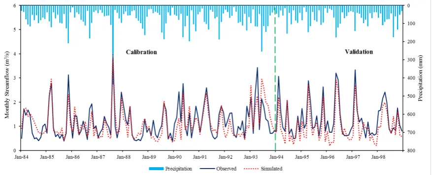
At the UWBDR, the total observed and simulated streamflow during the calibration period were 7.52 m3/s and 7.60 m3/s, respectively. The resulting hydrograph from SWAT streamflow in the
UWBDR also showed agreement in trends between the two (Figure 7). The best calibration achieved was an R2 of 0.69, PBIAS of 4.86, ENS of 0.67 and KGE of 0.82. Note that KGE was used as an objective
function type in the SUFI-2 calibration and validation because it could be decomposed into three terms that represented the correlation, bias and relative variability between the measured and simulated values [64]. Hence, it allowed the simultaneous use of baseflow and streamflow in calibration and enabled comparison between different strategies. The summed observed and simulated streamflow during the validation period were 9.03 m3/s and 8.27 m3/s, respectively.
Streamflow validation showed a higher performance than the calibration with an R2 of 0.84, PBIAS
of 23.1, ENS of 0.68 and KGE of 0.67 (Table 8).
measures were evaluated to test the performance of baseflow predictions. The R2 for the calibration
period was 0.67, with a PBIAS of -1.08, ENS of 0.60 and KGE of 0.80 (Table 8). Figure 8 shows the results of model calibration and validation of baseflow at the UWBDR. Overall, there was reasonably good agreement between computed and simulated baseflow. Further, the model performance was validated using data for the subsequent time period. It was observed that the computed baseflow from the USGS streamflow values were reasonably close to the simulated ones. The evaluation indices R2, PBIAS, ENS and KGE were 0.79, 8.43, 0.58 and 0.79 for the baseflow of the validation
period, respectively.
In general, the results suggested that the SWAT model performed satisfactorily in the UWBDR watershed according to the criteria set by Moriasi et al. [52]. However, the model underestimated the simulated streamflow for the validation period at a monthly time step during low streamflow, which indicates that there may be uncertainty in the results of SWAT simulations for urban watersheds. The lower performance of the SWAT model in the UWBDR may be attributed to the fact that the climate data obtained from the main weather station were located outside the basin, and the distribution of the climate stations with a complete record was sparse. In addition, the overestimation of some peaks in baseflow could be related to the existence of the West Chicago Moraine outwash plain, creating circumstances that promote fast groundwater movement from the moraine through the outwash. Ratios of baseflow to the total annual streamflow were 55.3% and 60.8% for both measured and simulated streamflow, respectively. This discrepancy is acceptable because all of the separation methods of baseflow using different filters are subject to uncertainties [36].
Figure 7. Observed and simulated time series streamflow for the UWBDR watershed during calibration and validation periods
Unlike the UWBDR and the LEC watersheds in Aboelnour et al. [8], the baseflow proportion of the observed and simulated streamflow at the Walzem Creek watershed were 33.3% and 26.8%, respectively, which indicated that surface runoff was a major supply component for the stream. Figure 9 shows the comparison between the simulated and observed monthly streamflow for the calibration and validation periods. USGS records show that the total monthly streamflow for Walzem Creek was 18.7 m3/s, while the simulated one was 19.5 m3/s. However, streamflow was overestimated
for most of the light rainfall events (dry climate periods) and showed very good agreement with the large rainfall events (wet periods). Previous studies have shown that SWAT performed better under more humid climatic conditions [65,66]. In addition, SWAT has some problems with precisely accounting for water loss through infiltration and evapotranspiration, especially during dry climate seasons, and evaluating the soil moisture storage [67,68].
During the streamflow calibration period, the R2, ENS, PBIAS and KGE were 0.87, 0.87, -4.31 and
0.91, respectively, while they were 0.83, -3.83, 0.70 and 0.52 during the validation period (Table 8). The SWAT performance for the monthly streamflow during both the calibration and validation periods was very good [52]. Moreover, the high values of R2 and ENS in the calibration and validation
periods indicated that, with calibrated parameters, the SWAT model was useful to simulate streamflow in semi-arid regions and to further quantify the hydrological impacts of climate variation and land use change over water balance components. Although the SWAT performance for the streamflow validation period was not as good as the calibration period, results showed that its performance was still good, implying that SWAT is applicable to Walzem Creek. The reason that SWAT validation performance was less than the calibration performance is most likely due to the occurrence of an extreme flooding event in October 1998, in which a strong flood killed at least 25 people and caused hundreds of millions of dollars in damages across counties in the southern and eastern regions of San Antonio. The SWAT model poorly matched the peak flow of this large event.
Results also indicated that the simulated values of baseflow were slightly lower than those of the computed ones from observed USGS records. The computed monthly baseflow from USGS records and the simulated one were 6.23 m3/s and 5.22 m3/s, respectively, during the whole calibration
and validation periods. Figure 10 shows the comparison between the simulated and the computed monthly baseflow values at the Walzem Creek watershed in the calibration and validation periods. In the calibration period, the baseflow of the computed and simulated results had a similar trend. Meanwhile, the values of R2, ENS, PBIAS and KGE were 0.85, 21.65, 0.76 and 0.70, respectively, with
a P-factor of 70% and R-factor of 0.62. In the validation period, these measures were 0.70, -5.12, 0.68 and 0.79, respectively. The statistical measure results indicated a ‘very good’ to ‘good’ match between the simulated baseflow in the calibration and validation periods and the computed records [52]. However, SWAT overestimated the computed baseflow during the validation period, which was exemplified in the negative values of PBIAS. The statistical indicator and the similar trend between the computed and simulated results showed that the SWAT model was adequate in the semi-arid region of Walzem Creek, and confirmed that the optimized and calibrated model can be applied to evaluate the responses of the basin’s hydrology to land use and climate change.
Figure 9. Observed and simulated time series streamflow for the Walzem Creek watershed during calibration and validation periods
Figure 10. Observed and simulated time series baseflow for the Walzem Creek watershed during calibration and validation periods
Table 8. Statistical indicators for calibration and validation periods for streamflow and baseflow in the UWBDR watershed and Walzem Creek watershed
Period Streamflow (m3/s) Baseflow (m3/s)
R2 ENS PBIAS KGE R2 ENS PBIAS KGE
UWBDR Calibration (1984-1993) 0.69 0.67 4.9 0.82 0.67 0.60 -1.1 0.80 Validation (1994-1998) 0.84 23.09 0.7 0.67 0.79 0.58 8.4 0.79 Walzem Calibration (1984-1993) 0.87 0.87 Validation (1994-1998) 0.83 0.70 -4.3 -3.8 0.91 0.85 0.76 0.54 0.70 0.68 -5.12 0.79 21.6 0.70
3.5. Impacts of land use change
It was observed that baseflow increased by 2 mm (accounting for 3.0%) when only the effect of land use dynamics between the two different periods was considered.
Figures 11 and 12 show the distribution of the monthly average water yield and baseflow simulated by SWAT, respectively, for the four scenarios for the UWBDR. We observed that the average monthly water yield was concentrated in the late fall/spring seasons and accounted for 29% in the land use change scenario (X2). The change in water yield tended to be positive under the X2 scenario except for the winter season. On the other hand, land use change had minimal effect on baseflow, with no obvious change between X1 and X2. Baseflow variation showed increasing trends in warm months from May to September, then decreased from October to April. Such increase may be attributed to leakage from an outwash plain at the base of West Chicago Moraine and the increased precipitation during the wet season.
The results in Table 10 show that the average annual water yield increased by 15.5% due to the urbanization effect in Walzem Creek (X2-X1). Meanwhile, urbanization caused the baseflow to experience a dramatic increase by 186.8%. Based on the proposed approach, the average annual evapotranspiration and surface runoff variability during the three scenarios were further analyzed to provide deeper insight into how climate and land use dynamics interacted with hydrologic systems in Walzem Creek watershed. In semi-arid regions, hydrologic systems could be very sensitive to climate variability. Evapotranspiration was an important component of the hydrologic process, often nearly equaling precipitation in the catchment water balance, and under given climate conditions, it was mainly affected by vegetation cover [69]. Under the same precipitation conditions, decreased evapotranspiration brought an increase in baseflow and streamflow, while increased evapotranspiration led to the reduction in both [70]. This is illustrated in our finding shown in Table 12, in which evapotranspiration experienced a reduction by 2.4% due to the land use alteration.
Figure 13 illustrates the monthly impacts of land use change, climate and their joint effect on Walzem Creek’s water yield. Land use change had a more pronounced effect for all months in conjunction with a higher monthly average of rainfall in the first period of time (TS1). For example, the monthly average precipitation in June was 120.2 mm in TS1, and decreased to 75.0 mm in TS2. The contribution of land use impacts on monthly water yield were the highest in February, June, October, and December. Conversely, deforestation and urban expansion resulted in a major increase in monthly baseflow in all months from January to July with a total of 68.8% (Figure 14).
Table 9. Average annual change in water yield and baseflow in the UWBDR watershed.
Scenario Land Use Climate Water Yield (mm) Baseflow (mm) Evapotranspiration (mm) Surface Runoff (mm)
Av. Ch. Δ (%) Av. Ch. Δ (%) Av. Ch. Δ (%) Av. Ch. Δ (%)
X1 1992 TS1 312.6 - - 65.9 - - 568.6 - - 238.3 - -
X2 2011 TS1 314.1 1.5 0.5 67.9 2.0 3.0 567.8 -0.8 -0.1 240.86 2.59 1.1 X3 1992 TS2 343.4 30.8 9.9 119.7 53.8 81.6 608.6 40 7.0 265.24 26.97 11.3 X4 2011 TS2 347.1 34.6 11.1 73.0 7.1 10.8 605.2 36.6 6.4 268.38 30.11 12.6
Table 10. Average annual change in water yield and baseflow in Walzem Creek watershed.
Scenario Land Use Climate Water Yield (mm) Baseflow (mm) Evapotranspiration (mm) Surface Runoff (mm)
Av. Ch. Δ (%) Av. Ch. Δ (%) Av. Ch. Δ (%) Av. Ch. Δ (%)
X1 1992 TS1 289.2 - - 30.5 - - 541.3 - - 252.2 - -
X2 2011 TS1 334.1 44.9 15.5 87.3 56.9 186.8 520 -21.3 -3.9 239.5 -12.7 -5.0 X3 1992 TS2 291.8 2.70 0.9 82.2 51.7 169.9 514.9 -26.4 -4.9 202.6 -49.6 -19.7 X4 2011 TS2 300.5 11.3 3.9 74.6 44.1 144.9 505.1 -36.2 -6.7 219.1 -33.0 -13.1
Figure 11. Monthly water yield change for the UWBDR watershed under different scenarios
3.6. Impacts of climate variation
In comparison to the land use change scenario, the climate variation scenario caused the average annual water yield to increase by 9.9% as a result of a prominent increase in precipitation. Baseflow also showed an increase when only climate variation was considered (X3), however this increase was much more pronounced than the change in water yield, with an amount of 53.8 mm (81.6%) (Table 9). These results indicate that both land use change and climate variability played a role in increasing baseflow. However, climate change played a more pronounced role than land use change in impacting the hydrologic regime of the UWBDR during the recent past, due mainly to the increase in precipitation. This can also be seen in Table 9, in which the surface runoff and evapotranspiration increased by 11.3% and 7.0%, respectively. Together, these results indicate that the climate alteration contributes more substantially to the effects observed on hydrological components compared to urbanization.
Similar to the land use change scenario, the average monthly water yield was predominantly observed in late fall/spring. Of note, the highest change in monthly water yield is observed in July (39%) due to the X3 (climate change) scenario. The change in water yield tended to be positive in months that experienced a significant increase in precipitation in the second period (TS2) compared to the first one (TS1) (Figure 11). On the other hand, results showed an increase in average monthly baseflow under the effect of climate change only, impacts of S3 in all months, though the highest growth was detected in the warmest months of the year (May to September) (Figure 12).
The climate change scenario had a minimal impact on the average annual water yield, causing it to increase by only 0.9% at Walzem Creek, while it caused the average annual baseflow to increase by 169.9% (51.7 mm) compared to the baseline scenario (X1) (Table 10). This may be attributed to the significant reduction in the precipitation pattern and the increase in temperature in TS2 as compared to TS1, where the climate became warmer and drier. Therefore, these likely played an important role in the contribution to the total streamflow for Walzem Creek. Climatic variables, specifically precipitation, largely determined the runoff hydrograph. Precipitation reduction in the second climatic period (TS2) resulted in the significant decline of surface runoff by 49.6 mm (19.7%), and a reduction in evapotranspiration by 4.9%, within the X3 scenario (Table 10).
On a monthly basis, the highest impacts of climate change were detected in July, August and September, where the average monthly precipitation was higher in TS2 as compared to TS1. It could be inferred that climate variation had a lasting negative effect on water yield (Figure 13). However, the climate change scenario (X3) caused an increase in monthly baseflow from August to December by an amount of 43.9%. The increase of baseflow in the second half of the year was mainly due to changes in precipitation and temperature patterns from TS1 to TS2. For example, TS2 experienced less precipitation as compared to TS1, while the temperature was higher in TS2 compared to TS1. Hence, baseflow played a role in water contribution to total streamflow when the weather got warmer and drier in the semi-arid watershed (Figure 14).
the main contributor to the total streamflow considering the sole effect of climate variation at the Walzem Creek watershed.
Figure 13. Monthly water yield change for the Walzem Creek watershed under different scenarios
Figure 14. Monthly baseflow change for the Walzem Creek watershed under different scenarios
3.7. Combined impacts of both land use change and climate variations
impacts for the LEC watershed, in contrast to the significant positive effects of climate variation for the UWBDR watershed.
Similar to the climate scenario, we observed that the average monthly water yield was concentrated in the late fall and early spring in the X4 scenario, totaling 39% of the annual yield. In general, positive changes were detected in all months under different scenarios except for November, January and February. However, the variation due to the joint effects tended to be higher in all months with a higher precipitation pattern in the second period of time (TS2) than in TS1 (Figure 11). For instance, the effect of land use scenario (X2) was higher than those of X3 and X4 in August, as the average monthly rainfall was 127.2 mm in TS1, while it was only 99.8 mm in TS2. Meanwhile, the combined effect of land use change and climate variability and the sole effect of climate change had greater impacts on water yield in July, as the average monthly precipitation was 83.7 in TS1, increasing to 114.8 mm in TS2. Baseflow variations showed increasing trends in warm months from May to September, then decreased from October to April in conjunction with the joint effect of climate variation and land use change (Figure 12). The increase in baseflow may be mostly due to an increase in rainfall, and could be explained by fluctuations in both precipitation and temperature between TS1 and TS2. The freeze-thaw processes of the active layer could have changed the soil infiltration capacity and the volume of subsurface water storage, thus impacting baseflow as well [71].
Results from the X4 scenario in the Walzem Creek watershed indicate that the average annual water yield increased by only 3.9%, while the average annual baseflow showed a significant increase of 144.9% (Table 10). Additionally, the annual evapotranspiration was negatively impacted by the joint effect of climate variation and land use change, decreasing by 6.7%. The decline in evapotranspiration is mainly caused by reduction in green cover (Table 7). Compared to X1, the combined effects of land use change and climate variability under X4 decreased surface runoff by 33.0 mm (13.1%). Therefore, with the decline in precipitation and increase in water yield, baseflow was the predominant contributor to the total streamflow in Walzem Creek. These findings indicate that, with the concurrent reduction in evapotranspiration, average annual water yield and baseflow had a remarkable increase under the X4 scenario. However, the joint effect of climate variability and land use change on water yield and baseflow was lower than the sole impact of the land use change scenario. On the other hand, X4 had the greatest negative impact on evapotranspiration. Furthermore, on a monthly basis, the contribution of the joint effect of both climate variability and land use change tended to be similar to the contribution of climate change impacts. Therefore, it should be noted that the impact of land use change was the dominant contributor to both water yield and baseflow expansion for Walzem Creek, and was greater than the sole effects of climate change and the combined effects of land use and climate change.
At a monthly timescale, the streamflow increased in January, July, August, September and November for all three scenarios, with the highest increase in November by 66.5% (X2), 85.13% (X3), and 89.4% (X4). Note that streamflow in Walzem Creek showed a significant increase in all months when considering the impacts of land use change (X2), except for May and a minor reduction in October (Figure 16), which was caused by the reduction in rainfall and the insignificant increase of temperature for these months. Moreover, the streamflow rate tended to decrease when considering scenarios X3 and X4, except in January, July, August, September and November, due to the increase in precipitation during these months. The impact of the combined effect of land use change and climate variability showed the same behaviors as the sole impact of climate variability in the Walzem Creek watershed. This situation is well demonstrated by the monthly streamflow variation in the watershed (Figure 16), with the greatest streamflow increase estimated in September by 92.8%. Meanwhile, the highest reduction in monthly streamflow when considering the combined impacts was estimated in June by 22.35%. These changes were mainly the result of incremental, dynamic precipitation patterns between the two periods, TS1 and TS2. For instance, September experienced the highest increase in rainfall with an amount of 40.4 mm, while June showed the highest reduction in monthly precipitation with an amount of 45.2 mm in TS2 as compared to TS1.
land use change and climate change had an impact on streamflow and baseflow. However, our study showed that land use dynamics and urban expansion played a more important role on streamflow and baseflow in semi-arid regions than solely climate change impacts.
Figure 15. Absolute change in mean monthly streamflow for the UWBDR watershed under different scenarios.
Figure 16. Absolute change in mean monthly streamflow for the Walzem Creek watershed under different scenarios.
4. Summary and Conclusions
Urbanization and climate change play an important role in altering the spatiotemporal distribution of water resources and hydrologic components. Streamflow and baseflow are two critically important components of hydrology that are essential to sustain water demands by various sectors, such as agriculture and industry, and are vulnerable to these changes. Therefore, it is of vital significance to understand the behaviors of these components under the separate and combined impacts of climate variation and land use dynamics in different climate regions. In this research, we followed the methodology discussed by Aboelnour et al. [8] for computing streamflow and baseflow for diverse watersheds.
break point and the trends in hydrological and meteorological components. The SWAT model exhibited high-quality results for calibrating and validating models in the selected watersheds as indicated by evaluation criteria, and proved versatile in modeling the effects of environmental change in complex catchments. In addition, the automated SUFI-2 approach helped in minimizing the discrepancies between the observed and simulated data.
Findings of this research indicated that the climate became warmer and wetter for both the UWBDR and LEC watersheds evaluated in Aboelnour et al. [8] but warmer and drier at the Walzem Creek watershed. The combined effect of these changes showed nonlinear responses to the water balance component. Changes at the UWBDR watershed were remarkably similar to those for the LEC watershed, with the exception that the climate variation was shown to have the greater impact on both streamflow and baseflow, while land use change exerted a relatively small influence on either flow. On the other hand, urbanization influenced streamflow and baseflow in the semi-arid Walzem Creek watershed, possibly because of the change in rainfall pattern between the two climate periods. The small reduction in mean annual precipitation in the TS2 produced a considerable reduction in runoff.
Generally, with the variation in spatio-temporal properties of precipitation, and increasing hazardous events associated with water, such as droughts and floods, stress on water resources will increase and will further encourage the development of mitigation approaches. Based on this research, findings will provide practical suggestions for policy makers on how to sustain water resources more efficiently in relation to its variability as a response to urbanization, land use and climate change. These changes can be problematic and incur great cost to establish new infrastructure, especially in undeveloped nations. Therefore, policy makers need to develop policies to address these types of changes, taking into account the individual influences of human activities and climate variation, for instance, improving infrastructure to be more resilient to human activities, constructing dams following proper regulations on water resources, and limiting the amount of deforestation, which threatens some hydrological components. In addition, outcomes of this study can be used in quantifying the potential impacts of future projected climate change and land use change. Nevertheless, it might be found that the driving factors interact to impact streamflow and baseflow through chain effects, in which one factor is trying to increase/decrease the magnitude of the other. Hence, more studies are crucial to evaluate this potential future impact on the hydrological system, with the emphasis on the interactive effect of environmental change drivers when predicting future change.
While this research showed the separate and combined impacts of human activity and climate alteration using the SWAT model, modelers should be aware that other types of uncertainties associated with the model exist that may result from observed data, the parameterization process, or from the conceptual model itself. One of the potential shortcomings of this study is that the urbanization processes is an integrated part of the watershed, along with climate alteration. Therefore, it is difficult to discern whether the separate effects of human action and climate change were able to be truly simulated and this issue might therefore create a biased condition. Thus, a suggestion to avoid this limitation in future research is to hypothesize an extreme land use/land cover change that is sensitive to the change instead of a natural system simulated by the model.
Author Contributions: Writing original draft, M.A; Methodology, M.A. and M.W.G; Formal analysis, M.A and B.E; Editing-review M.W.G and B.E.; Conceptualization M.W.G; Supervision B.E.
Funding: This research was funded by Egyptian Government General Scholarship Programme (Ministry of Higher Education), administrated by the Egyptian Cultural and Education Bureau, Washington, DC, USA (Call 2013/2014)
Acknowledgments The authors would like to thank Celena Alford and Erin Sorlien for their critical reviews of the manuscript, and the Egyptian Government for financial support through the General Scholarship Program.
Conflicts of Interest: The authors declare no conflict of interest.
1. Ficklin, D.L.; Robeson, S.M.; Knouft, J.H. Impacts of recent climate change on trends in baseflow and stormflow in United States watersheds. Geophys. Res. Lett.2016, 43, 5079–5088.
2. Zhang, D.; Liu, X.; Liu, C.; Bai, P. Responses of runoff to climatic variation and human activities in the Fenhe River, China. Stoch. Environ. Res. Risk Assess.2013, 27, 1293–1301.
3. Tong, S.T.Y.; Sun, Y.; Ranatunga, T.; He, J.; Yang, Y.J. Predicting plausible impacts of sets of climate and land use change scenarios on water resources. Appl. Geogr.2012, 32, 477–489.
4. Duan, W.; He, B.; Nover, D.; Fan, J.; Yang, G.; Chen, W.; Meng, H.; Liu, C. Floods and associated socioeconomic damages in China over the last century. Nat. Hazards2016, 82, 401–413.
5. Zhang, Y.K.; Schilling, K.E. Increasing streamflow and baseflow in Mississippi River since the 1940 s: Effect of land use change. J. Hydrol.2006, 324, 412–422.
6. Kumar, S.; Merwade, V.; Kam, J.; Thurner, K. Streamflow trends in Indiana: Effects of long term persistence, precipitation and subsurface drains. J. Hydrol.2009, 374, 171–183.
7. Aboelnour, M.; Engel, B.A. Responses of Streamflow and Baseflow Hydrology to Climate Variability and Land Use Dynamics in an Urban Watershed. In Proceedings of the AGU Fall Meeting Abstracts; 2018.
8. Aboelnour, M.; Engel, B.A.; Gitau, M.W. Hydrologic Response in an Urban Watershed as A ff ected by Climate and Land-Use Change. Water (Switzerland)2019, 11, 1603.
9. Abdi, R.; Yasi, M. Evaluation of environmental flow requirements using eco-hydrologic-hydraulic methods in perennial rivers. Water Sci. Technol.2015, 72, 354–363.
10. Jin, H.; Zhu, Q.; Zhao, X.; Zhang, Y. Simulation and prediction of climate variability and assessment of the response of water resources in a typical watershed in china. Water (Switzerland)2016, 8, 490. 11. Novotny, E. V.; Stefan, H.G. Stream flow in Minnesota: Indicator of climate change. J. Hydrol.2007, 334,
319–333.
12. Frans, C.; Istanbulluoglu, E.; Mishra, V.; Munoz-Arriola, F.; Lettenmaier, D.P. Are climatic or land cover changes the dominant cause of runoff trends in the Upper Mississippi River Basin? Geophys. Res. Lett.
2013, 40, 1104–1110.
13. Duan, W.; He, B.; Takara, K.; Luo, P.; Nover, D.; Hu, M. Impacts of climate change on the hydro-climatology of the upper Ishikari river basin, Japan. Environ. Earth Sci.2017, 76, 1–16.
14. Chen, J.; Theller, L.; Gitau, M.W.; Engel, B.A.; Harbor, J.M. Urbanization impacts on surface runoff of the contiguous United States. J. Environ. Manage.2017, 187, 470–481.
15. Xu, X.; Scanlon, B.R.; Schilling, K.; Sun, A. Relative importance of climate and land surface changes on hydrologic changes in the US Midwest since the 1930s: Implications for biofuel production. J. Hydrol.
2013, 497, 110–120.
16. Gebert, W.A.; Radloff, M.J.; Considine, E.J.; Kennedy, J.L. Use of streamflow data to estimate base flowground-water recharge for Wisconsin. J. Am. Water Resour. Assoc.2007, 43, 220–236.
17. Neff, B.P.; Day, S.M.; Piggott, A.R.; Fuller, L.M. Base flow in the Great Lakes basin. U.S. Geol. Surv. Sci. Investig. Rep.2005, 32.
18. Charles, D. Assessing regional land-use/cover influences on New Jersey Pinelands streamflow through hydrograph analysis. Hydrol. Process.2007, 21, 185–197.
19. King, R.S.; Scoggins, M.; Porras, A. Stream biodiversity is disproportionately lost to urbanization when flow permanence declines: Evidence from southwestern North America. Freshw. Sci.2016, 35, 340–352. 20. Price, K.; Jackson, C.R.; Parker, A.J.; Reitan, T.; Dowd, J.; Cyterski, M. Effects of watershed land use and
geomorphology on stream low flows during severe drought conditions in the southern Blue Ridge Mountains, Georgia and North Carolina, United States. Water Resour. Res.2011, 47.
21. Price, K. Effects of watershed topography, soils, land use, and climate on baseflow hydrology in humid regions: A review. Prog. Phys. Geogr.2011, 35, 465–492.
22. Dey, P.; Mishra, A. Separating the impacts of climate change and human activities on streamflow: A review of methodologies and critical assumptions. J. Hydrol.2017, 548, 278–290.
23. Khoi, D.N.; Thom, V.T. Impacts of climate variability and land-use change on hydrology in the period 1981-2009 in the central highlands of vietnam. Glob. Nest J.2015, 17, 870–881.
24. Li, Z.; Liu, W. zhao; Zhang, X. chang; Zheng, F. li Impacts of land use change and climate variability on hydrology in an agricultural catchment on the Loess Plateau of China. J. Hydrol.2009, 377, 35–42. 25. Jothityangkoon, C.; Sivapalan, M.; Farmer, D.L. Process controls of water balance variability in a large
semi-arid catchment: Downward approach to hydrological model development. J. Hydrol.2001, 254, 174–198.
26. Gitau, M.W.; Chaubey, I. Regionalization of SWAT Model Parameters for Use in Ungauged Watersheds. Water2010, 2, 849–871.
Part I: Model development. JAWRA J. Am. Water Resour. Assoc.1998, 34, 73–89.
28. Liu, G.; He, Z.; Luan, Z.; Qi, S. Intercomparison of a lumped model and a distributed model for
streamflow simulation in the Naoli River Watershed, Northeast China. Water (Switzerland)2018, 10. 29. Arnold, J.G.; Moriasi, D.N.; Gassman. P. W; Abbaspour, K.C.; White, M.J.; Srinivasan, R.; Santhi, C.;
Harmel, R.D.; Van Griensven, A.; Van Liew, M.W.; et al. SWAT: Model Use, Calibration, and Validation. Trans. ASABE2012, 55, 1491–1508.
30. Neitsch, S..; Arnold, J..; Kiniry, J..; Williams, J.. Soil and Water Assessment Tool Theoretical Documentation - Version 2009, Technical Report no 406. 2009, 618.
31. Abbaspour, K.C.; Rouholahnejad, E.; Vaghefi, S.; Srinivasan, R.; Yang, H.; Kløve, B. A continental-scale hydrology and water quality model for Europe: Calibration and uncertainty of a high-resolution large-scale SWAT model. J. Hydrol.2015, 524, 733–752.
32. Zhang, X.; Srinivasan, R.; Arnold, J.; Izaurralde, R.C.; Bosch, D. Simultaneous calibration of surface flow and baseflow simulations: A revisit of the SWAT model calibration framework. Hydrol. Process.2011, 25, 2313–2320.
33. Luo, Y.; Arnold, J.; Allen, P.; Chen, X. Baseflow simulation using SWAT model in an inland river basin in Tianshan Mountains, Northwest China. Hydrol. Earth Syst. Sci.2012, 16, 1259–1267.
34. Yan, T.; Bai, J.; Lee Zhi Yi, A.; Shen, Z. SWAT-simulated streamflow responses to climate variability and human activities in the Miyun Reservoir basin by considering streamflow components. Sustain.2018, 10. 35. Mwakalila, S.; Feyen, J.; Wyseure, G. The influence of physical catchment properties on baseflow in
semi-arid environments. J. Arid Environ.2002, 52, 245–258.
36. Zhang, L.; Nan, Z.; Xu, Y.; Li, S. Hydrological impacts of land use change and climate variability in the headwater region of the Heihe River Basin, northwest China. PLoS One2016, 11, 1–25.
37. Burke, C.B.; West, E.; Street, W.M.; Charles, S.; Burke, C.B. West branch dupage river watershed plan; 2006; Vol. 60174;.
38. Hejazi, M.I.; Markus, M. Impacts of Urbanization and Climate Variability on Floods in Northeastern Illinois. J. Hydrol. Eng.2009, 14, 606–616.
39. Clean River Program San Antonio River Basin Watershed Characterizations for the Upper San Antonio River, Salado Creek and Upper Cibolo Creek Watersheds; 2017;
40. Drury, B.; Rosi-Marshall, E.; Kelly, J.J. Wastewater treatment effluent reduces the abundance and diversity of benthic bacterial communities in urban and suburban rivers. Appl. Environ. Microbiol.2013, 79, 1897–1905.
41. Kottek, M.; Grieser, J.; Beck, C.; Rudolf, B.; Rubel, F. World map of the Köppen-Geiger climate classification updated. Meteorol. Zeitschrift2006.
42. Mehan, S.; Neupane, R.P.; Kumar, S. Coupling of SUFI 2 and SWAT for Improving the Simulation of Streamflow in an Agricultural Watershed of South Dakota. Hydrol. Curr. Res.2017, 8.
43. Jung, Y.; Shin, Y.; Won, N. Il; Lim, K.J. Web-based BFlow system for the assessment of streamflow characteristics at national level. Water (Switzerland)2016, 8.
44. Lee, J.; Kim, J.; Jang, W.S.; Lim, K.J.; Engel, B.A. Assessment of baseflow estimates considering recession characteristics in SWAT. Water (Switzerland)2018, 10, 1–14.
45. Eckhardt, K. A comparison of baseflow indices, which were calculated with seven different baseflow separation methods. J. Hydrol.2008, 352, 168–173.
46. Hamed, K.H.; Rao, R.A. A modified Mann-Kendall trend test for autocorrelated data. J. Hydrol.1998, 204, 182–196.
47. Abbaspour, K.C. SWAT-CUP: SWAT Calibration and Uncertainty Programs; 2015; Vol. 130;.
48. Welde, K.; Gebremariam, B. Effect of land use land cover dynamics on hydrological response of
watershed: Case study of Tekeze Dam watershed, northern Ethiopia. Int. Soil Water Conserv. Res.2017, 5, 1–16.
49. Ghazal, K.A.; Leta, O.T.; El-Kadi, A.I.; Dulai, H. Assessment of wetland restoration and climate change impacts on water balance components of the Heeia coastalwetland in Hawaii. Hydrology2019, 6. 50. T. L. Veith; M. W. Van Liew; D. D. Bosch; J. G. Arnold Parameter Sensitivity and Uncertainty in SWAT:
A Comparison Across Five USDA-ARS Watersheds. Trans. ASABE2010.
51. Yuan, E.; Nie, W.; Sanders, E. Problems and Prospects of SWAT Model Application on an Arid/Semi-arid Watershed in Arizona. SEDHYD 2014 Jt. Conf.2015.
52. Moriasi, D.N.; Arnold, J.G.; Van Liew, M.W.; Bingner, R.L.; Harmel, R.D.; Veith, T.L. Model Evaluation
Guidelines for Systematic Quantification of Accuracy in Watershed Simulations. Trans. ASABE2007, 50, 885–900.
54. Nie, W.; Yuan, Y.; Kepner, W.; Nash, M.S.; Jackson, M.; Erickson, C. Assessing impacts of Landuse and Landcover changes on hydrology for the upper San Pedro watershed. J. Hydrol.2011, 407, 105–114. 55. Moriasi, D.N.; Gowda, P.H.; Arnold, J.G.; Mulla, D.J.; Ale, S.; Steiner, J.L.; Tomer, M.D. Evaluation of the
Hooghoudt and Kirkham Tile Drain Equations in the Soil and Water Assessment Tool to Simulate Tile Flow and Nitrate-Nitrogen. J. Environ. Qual.2013, 42, 1699.
56. Thirel, G.; Andréassian, V.; Perrin, C.; Audouy, J.N.; Berthet, L.; Edwards, P.; Folton, N.; Furusho, C.; Kuentz, A.; Lerat, J.; et al. Hydrologie sous changement: un protocole d’évaluation pour examiner comment les modèles hydrologiques s’accommodent des bassins changeants. Hydrol. Sci. J.2015, 60, 1184–1199.
57. Sen, P.K. Estimates of the Regression Coefficient Based on Kendall’s Tau. J. Am. Stat. Assoc.1968, 63, 1379–1389.
58. Hirsch, R.M.; Slack, J.R.; Smith, R.A. Techniques of trend analysis for monthly water quality data. Water Resour. Res.1982, 18, 107–121.
59. Bhaskar, A.S.; Beesley, L.; Burns, M.J.; Fletcher, T.D.; Hamel, P.; Oldham, C.E. Will it rise or will it fall ? Managing the complex e ff ects of urbanization on base fl ow. 2016, 35, 293–310.
60. Sekaluvu, L.; Zhang, L.; Gitau, M. Evaluation of constraints to water quality improvements in the Western Lake Erie Basin. J. Environ. Manage.2018, 205, 85–98.
61. Aboelnour, M.; Engel, B.A. Application of Remote Sensing Techniques and Geographic Information Systems to Analyze Land Surface Temperature in Response to Land Use/Land Cover Change in Greater Cairo Region, Egypt. J. Geogr. Inf. Syst.2018, 10, 57–88.
62. Gitau, M.; Bailey, N. Multi-Layer Assessment of Land Use and Related Changes for Decision Support in a Coastal Zone Watershed. Land2012, 1, 5–31.
63. Castilla, G.; Hay, G.J. Uncertainties in land use data. Hydrol. Earth Syst. Sci.2007, 11, 1857–1868.
64. Lazzari Franco, A.C.; Bonumá, N.B. Multi-variable SWAT model calibration with remotely sensed
evapotranspiration and observed flow. Rev. Bras. Recur. Hídricos - Brazilian J. Water Resour.2017, 22, ISSN 2318-0331.
65. Liew, M.W. Van; Arnold, J.G.; Bosch, D.D. Problem and Potential of Autocalibrating a Hydrlogic Model. Trans. ASABE2005, 48, 1025–1040.
66. Van Liew, M.W.; Veith, T.L.; Bosch, D.D.; Arnold, J.G. Suitability of SWAT for the Conservation Effects Assessment Project: Comparison on USDA Agricultural Research Service Watersheds. J. Hydrol. Eng.
2007, 12, 173–189.
67. Feyereisen, G.W.; Strickland, T.C.; Bosch, D.D.; Sullivan, D.G. Evaluation of SWAT Manual Calibration and Input Parameter Sensitivity in the Little River Watershed. Trans. Am. Soc. Agric. Biol. Eng.2007, 50, 843–856.
68. Tobin, K.J.; Bennett, M.E. Using SWAT to model streamflow in two river basins with ground and satellite precipitation data. J. Am. Water Resour. Assoc.2009, 45, 253–271.
69. Zhang, L.; Karthikeyan, R.; Bai, Z.; Srinivasan, R. Analysis of streamflow responses to climate variability and land use change in the Loess Plateau region of China. Catena2017, 154, 1–11.
70. Schilling, K.E.; Jha, M.K.; Zhang, Y.-K.; Gassman, P.W.; Wolter, C.F. Impact of land use and land cover change on the water balance of a large agricultural watershed: Historical effects and future directions. Water Resour. Res.2008, 44, 1–12.
71. Qin, J.; Ding, Y.; Han, T.; Liu, Y. Identification of the factors influencing the baseflow in the permafrost

![Table 1. SWAT input parameters used for the UWBDR and Walzem Creek watersheds calibration of streamflow and baseflow [8]](https://thumb-us.123doks.com/thumbv2/123dok_us/1089215.1609508/6.595.79.519.203.529/table-parameters-uwbdr-walzem-watersheds-calibration-streamflow-baseflow.webp)