Data-Informed Decomposition for Localized Uncertainty Quantification of Dynamical Systems

(1)

Article

Data-Informed Decomposition for Localized

Uncertainty Quantification of Dynamical Systems

Waad Subber˚_{, Sayan Ghosh, Piyush Pandita, Yiming Zhang and Liping Wang}

1 2 3 4

5 6 7 8

9 10 11

12 13 14 15

16 17 18 19

20

ProbabilisticDesignandOptimizationGroup,GEResearch,1ResearchCircle,Niskayuna,NY12309,USA * Correspondence:[email protected]

Abstract: Industrial dynamical systems often exhibit multi-scale response due to material

heterogeneities, operation conditions and complex environmental loadings. In such problems, it is the

case that the smallest length-scale of the systems dynamics controls the numerical resolution required

to effectively resolve the embedded physics. In practice however, high numerical resolutions is only

required in a confined region of the system where fast dynamics or localized material variability are

exhibited, whereas a coarser discretization can be sufficient in the rest majority of the system. To

this end, a unified computational scheme with uniform spatio-temporal resolutions for uncertainty

quantification can be very computationally demanding. Partitioning the complex dynamical system

into smaller easier-to-solve problems based of the localized dynamics and material variability can

reduce the overall computational cost. However, identifying the region of interest for high-resolution

and intensive uncertainty quantification can be a problem dependent. The region of interest can be

specified based on the localization features of the solution, user interest, and correlation length of

the random material properties. For problems where a region of interest is not evident, Bayesian

inference can provide a feasible solution. In this work, we employ a Bayesian framework to update

our prior knowledge on the localized region of interest using measurements and system response. To

address the computational cost of the Bayesian inference, we construct a Gaussian process surrogate

for the forward model. Once, the localized region of interest is identified, we use polynomial

chaos expansion to propagate the localization uncertainty. We demonstrate our framework through

numerical experiments on a three-dimensional elastodynamic problem.

Keywords: Bayesian inference; Uncertainty Quantification; Dynamical Systems; Inverse Problem;

System Identification ; Gaussian process regression; Polynomial chaos.

21

1. Introduction

22

With the increase in demand for high-performance and highly-efficiency systems, the complexity

23

of industrial design and manufacturing process is increasing proportionally; exposing many

24

opportunities for novel technologies as well as many associated technical challenges. For example,

25

advancements in the design of composite structures allows us to reduce weight, advancements in

26

additive manufacturing enables us to reduce cost, and optimal computational material design pushes

27

the boundary in the discovery of new alloys with desirable electro-mechanical properties. Introducing

28

a new technology typically happens at the lowest level of the systems hierarchy (e.g., at the parts or

29

sub-component levels). Extending the new technologies to the system level requires rigorous testing.

30

For example, in 1980’s composite material was only used for limited components of an aircraft (i.e,.

31

the wing and tail [1]). Recently however, after multiple test flights, about 50% of the materials used in

32

the Boeing 787 Dreamliner are composite materials [2].

33

In the industrial setting, the process of adaptation of a new technology can be accelerated by a

34

proper assessment of uncertainty at various aspects of the product ’s life cycle spanning the design,

35

manufacturing and maintenance stages. For example, at the design stage of an aircraft wing rib, it

36

is crucial to consider the effect of uncertainty in the material and operation conditions on the safety

37

factor and aeroelastic dynamics of the wing [3]. At the manufacturing stage, it is important to consider

38

Preprints (www.preprints.org) | NOT PEER-REVIEWED | Posted: 17 August 2020 doi:10.20944/preprints202008.0358.v1

(2)

the impact of manufacturing uncertainties on quality control [4] and non-destructive testing [5]. The

39

maintenance stage requires a holistic assessment of the effect of measurement uncertainty on the static

40

and dynamic responses of the wing during structural health monitoring [6].

41

Quantifying uncertainty at the system level often requires a physics-based computational model

42

for the entire structure. However, in structures such as an aircraft wing, traditional computational

43

models may become too complex and costly for simulating the multi-scale dynamical response

44

especially due to material heterogenity at the sub-component level. The effect of the sub-component

45

on the entire structure depends on the size, location and loading conditions of the part. It is therefore,

46

necessary to consider a different level of fidelity for the analysis of the sub-components in order to

47

reduce the cost and complexity of uncertainty quantification. To this end, the concept of localized

48

uncertainty propagation for dynamical systems having muti spatio-temporal scales can be utilized to

49

address such issues [7–9].

50

In this work, we consider assessing the effect of localized uncertainty in a region of interest

51

within the entire structure. For structures composed of distinct parts that can be clearly identified,

52

the localized region for uncertainty propagation may become obvious. When the distinguished

53

components of a structure are not clear, measurement data can be utilized within Bayesian framework

54

to identify the localized region of interest. The Bayesian paradigm integrates thedomain-knowledge,

55

physics-based computational models and observational data in one framework to update the current

56

state of knowledge [10,11]. The Bayesian methods offer two major advantages namely: a) allow

57

quantification of epistemic uncertainty under limited-data, and b) retain physical sense for the

58

parameters and the quantity-of-interest. Conditioning apriori physics beliefs on the available data,

59

Bayes rule provides aposteriori distribution on the model parameters. A robust method to estimate

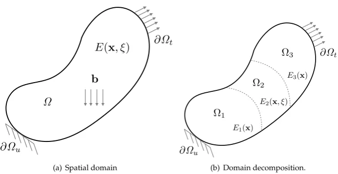
60

the posterior distribution in the Bayesian inference (i.e. sampling values of the model parameters from

61

the posterior probability) is Markov Chain Monte Carlo (MCMC) [12,13]. Estimating the posterior

62

probability density function in the Bayesian method requires solving the forward model many times,

63

which may become challenging for limited computing resources. This issue is often addressed by

64

building a data-driven probabilistic surrogate model using Gaussian process (GP) regression [14].

65

Constructing a GP model requires executing the forward model only few number of times. The

66

GP models are non-parametric and Bayesian in nature, and they provide uncertainty bound on

67

their predictions. Nevertheless, for problems with stochastic field representation of the variability

68

in the propagation media, uncertainty quantification using GP models may become challenging for

69

general non-Gaussian description of the underlying random variability. Polynomial Chaos (PC), on

70

the other hand, provides an effective framework to represent and propagate an arbitrary random

71

variable through complex computational models [15,16]. In PC, the response of the physical model is

72

represented as spectral expansion in a polynomial series with basis function being orthogonal with

73

respect to the probability density function of the underlying random variables of the propagation

74

media.

75

The rest of this work is organized as follows: in Section2, we provide the problem statement

76

and the associated mathematical formulations. Our numerical demonstrations for the mathematical

77

framework are provided in Section3. We provide the conclusions of the current work in Section4.

78

2. Methodology

79

In this section, we present the mathematical framework of our approach for data-driven

80

partitioning scheme for localized uncertainty quantification. In particular, in Subsection 2.1, we

81

introduce the problem statement in the Bayesian setting. As mentioned previously, for problems where

82

the localized region of interest is not defined explicitly, we rely on measurement data of a response

83

quantity (aided by a computational model) to infer the localized region of interest. The Bayesian

84

framework requires a computational model (the forward problem) to estimate the response of the

85

system for a given set of the input parameters that to be inferred. Consequently, in Subsection2.2

86

we discuss the stochastic elastodynamic problem and its finite element discretization. Estimating

(3)

3 of 16

the localized region of interest in the Bayesian setting necessitates many solutions to the stochastic

88

elastodynamic problem which can become computationally demanding. Furthermore, it is worth

89

noting that for the Bayesian calculation the entire solution field of the stochastic elastodynamic problem

90

is not required, only a realization at the measurement location is needed. Thus, a surrogate model

91

for the realization of the response can be used to reduce the computational cost of the Bayesian

92

framework. In Subsection2.3, we present the Gaussian process surrogate to emulate the solution to

93

the stochastic elastodynamic problem with less cost. Once the localized region of interest is estimated,

94

a confined uncertainty representation of the material properties within the region of interest can be

95

performed. The localized uncertainty is propagated forward through the model in order to estimate

96

its effect on the variability of the response. For this task, we use the polynomial chose expansion for

97

efficient assessment of uncertainty with less cost. The polynomial chose expansion is reviewed in

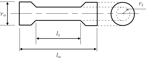
98

Subsection2.4.

99

2.1. Bayesian Inference

100

In Bayesian inference, the prior knowledge is updated to posterior using noisy measurements and the response of a physical model [10,11]. The update is based on the Bayes’ rule defined as

ppθ|dq “ ppθqppd|θq

ppdq , (1)

whereθis the uncertain parameters to be estimated,dis the measurement of an observable quantity,

ppθ|dqis the posterior probability density function,ppθqis the prior probability density function, and

ppd|θqdenotes the likelihood of the observations given the parameter. We assume that the measured

datadis generated from a statistical model composed of a physical modelMpθqplus an additive

measurements noiseeas

d“Mpθq `e. (2)

Here we represent the measurement noise as a Gaussian random variable with unknown variance

e„Np0,σ_n2q. For a Gaussian noise, the likelihood function becomes

ppd|θq “ 1

`

2πσ2

n

˘´N{2exp

˜

´ 1

2σ2

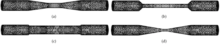
n N ÿ

i

rdi´Mpθiqs2

¸

. (3)

The task in hand is to utilize the measurementdand the physical modelMpθqto estimate the system

parametersθthat best satisfy Eq.(1). The process requires many executions to the physical modelMpθq,

which can be computationally expensive. It is often, the expensive computational model is emulated

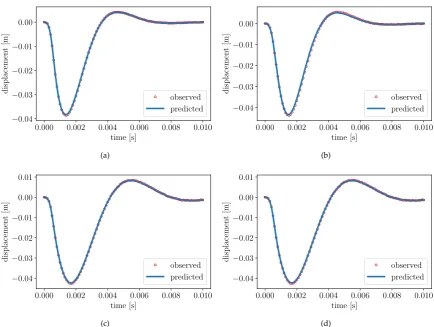
by a simplereasy-to-evaluatemodel that can estimate the response with a quantified accuracy as:

Mpθq »Mpθq, (4)

whereMpθqdenotes the surrogate model that is constructed using a limited runs of the physical model

101

Mpθq. In our work, we representMpθqas Gaussian process surrogate model [17]. Once we constructed

102

and validate the surrogate model, the parameterization of the localized featuresθis estimated using

103

Bayes’ rule evaluated by Markov Chain Monte Carlo (MCMC) sampling technique. Having the

104

localized region of interest identified, a localized uncertainty quantification of the confined variability

105

of the material properties can be performed efficiently using polynomial chaos expansion [15].

106

2.2. The Forward Problem

107

In this section, we give a brief summary of the mathematical formulation to the linear stochastic

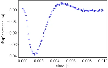
108

dynamical system considered in this work. The framework is presented for localized uncertainty

109

(4)

propagation work-flow, whereby the decomposition of the physical domain is based on the variability

110

of the material properties. Consequently, we consider an arbitrary physical domainΩP_RdwithBΩ

111

being its boundary as shown in Fig. (1-a), and define the following problem:

112

Find a random functionupx,t,ξq:Ωˆ r0,Tfs ˆΞÑR, such that the following equations hold

ρpξq:upx,t,ξq “ ∇¨σ`b in Ω ˆ r0,Tfs ˆΞ,

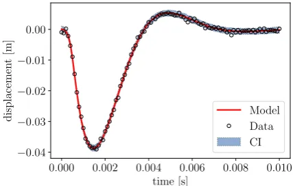
upx,t,ξq “ u¯ on BΩu ˆ r0,Tfs ˆΞ,

σ¨n“ ¯t on BΩt ˆ r0,Tfs ˆΞ,

upx, 0,ξq “ u0 in Ω ˆ Ξ,

9

upx, 0,ξq “ u90 in Ω ˆ Ξ,

(5)

whereρpξqis the mass density,σis the stress tensor,uis the displacement field,bis the body force

113

per unit volume, ¯uis the prescribed displacement onBΩu, ¯tis the prescribed traction onBΩt,nis a

114

unit normal to the surface, andu0andu90are the initial displacement and velocity, respectively. Here,

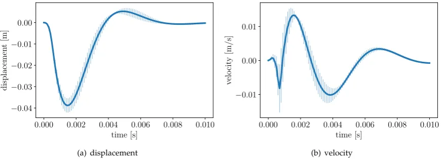
115

we define the stochastic space by (Θ,Σ,Pq, whereΘdenoting the sample space,Σbeing theσ-algebra

116

ofΘ, andPrepresenting an appropriate probability measure. The stochastic space is paramatrized

117

by a finite set of standardized identically distributed random variablesξ“ tξ_ipθqu_iM_“₁, whereθPΘ.

118

The support of the random variables is defined asΞ“Ξ1ˆΞ2ˆ ¨ ¨ ¨ΞMPRMwith a joint probability

119

density function given asppξq “p1pξ1q ¨p2pξ2q ¨ ¨ ¨pMpξMq.

120

For linear isotropic elastic martial, the constitutive relation between the stress and strain tensors is given by:

σ “λpξqtrpεqI`2¯pξqε, (6)

whereλpξqandµpξqare the Lemaé’s parameters,Iis an identity tensor andεis the symmetric strain

tensor defined as

ε“ 1

2 ´

∇u`∇uT

¯

. (7)

For a random Young’s modulusEpx,ξqand deterministic Poisson’s ratioν, the Lemaé’s parameters

can be expressed as

λpξq “ Epx,ξqν

p1`νqp1´2νq, µpξq “

Epx,ξq

2p1`νq. (8)

We consider the case that uncertainty steams from a localized variability in a confined region

121

within the physical domain. For example as shown in Fig. (1-b), the variability in the quantity of interest

122

can be attributed to the material random properties within the subdomainΩ2. The artificial martial

123

boundaries shown in Fig.(1-b) for subdomainΩ2is estimated using Bayesian inference. Localizing

124

random variability in the neighborhood of the quantity of interest reduces the computational cost

125

of uncertainty propagation in problems where a region of interest can be specified. Depending

126

on the interest in the region, each subdomain can have its local uncertainty representation and

127

the corresponding mesh and time resolutions. As a results the Asynchronous Space-Time Domain

128

Decomposition Method with Localized Uncertainty Quantification (PASTA-DDM-UQ) [7–9] can be

129

utilized. In PASTA-DDM-UQ, spatial, temporal and material decompositions are considered. In

130

this work however, we only consider material decomposition and apply non-intrusive approach for

131

uncertainty propagation.

132

Consequently, let the physical domainΩbe partitioned based on the martial variability intons

non-overlapping subdomainsΩs, 1ďsďnsas shown in Fig. (1-b) and such that:

Ω“

ns ď

s“1

Ωs, Ωsč

Ωr“ Hfors‰r, Γ“

ns ď

s“1

(5)

5 of 16

b

∂Ω

u

∂Ω

t

Ω

E(

x

, ξ)

(a) Spatial domain

@⌦u

@⌦t

⌦<latexit sha1_base64="2cHE4hOBMX049bWJt+9B26w2a/Y=">AAAB73icbVA9SwNBEJ2LXzF+RS1tFoNgFe5E0DJoY2cEEwPJEfY2c8mS3b1zd08IIX/CxkIRW/+Onf/GTXKFJj4YeLw3w8y8KBXcWN//9gorq2vrG8XN0tb2zu5eef+gaZJMM2ywRCS6FVGDgitsWG4FtlKNVEYCH6Lh9dR/eEJteKLu7SjFUNK+4jFn1Dqp1bmV2KfdoFuu+FV/BrJMgpxUIEe9W/7q9BKWSVSWCWpMO/BTG46ptpwJnJQ6mcGUsiHtY9tRRSWacDy7d0JOnNIjcaJdKUtm6u+JMZXGjGTkOiW1A7PoTcX/vHZm48twzFWaWVRsvijOBLEJmT5Pelwjs2LkCGWau1sJG1BNmXURlVwIweLLy6R5Vg38anB3Xqld5XEU4QiO4RQCuIAa3EAdGsBAwDO8wpv36L14797HvLXg5TOH8Afe5w+IR4+f</latexit><latexit sha1_base64="2cHE4hOBMX049bWJt+9B26w2a/Y=">AAAB73icbVA9SwNBEJ2LXzF+RS1tFoNgFe5E0DJoY2cEEwPJEfY2c8mS3b1zd08IIX/CxkIRW/+Onf/GTXKFJj4YeLw3w8y8KBXcWN//9gorq2vrG8XN0tb2zu5eef+gaZJMM2ywRCS6FVGDgitsWG4FtlKNVEYCH6Lh9dR/eEJteKLu7SjFUNK+4jFn1Dqp1bmV2KfdoFuu+FV/BrJMgpxUIEe9W/7q9BKWSVSWCWpMO/BTG46ptpwJnJQ6mcGUsiHtY9tRRSWacDy7d0JOnNIjcaJdKUtm6u+JMZXGjGTkOiW1A7PoTcX/vHZm48twzFWaWVRsvijOBLEJmT5Pelwjs2LkCGWau1sJG1BNmXURlVwIweLLy6R5Vg38anB3Xqld5XEU4QiO4RQCuIAa3EAdGsBAwDO8wpv36L14797HvLXg5TOH8Afe5w+IR4+f</latexit><latexit sha1_base64="2cHE4hOBMX049bWJt+9B26w2a/Y=">AAAB73icbVA9SwNBEJ2LXzF+RS1tFoNgFe5E0DJoY2cEEwPJEfY2c8mS3b1zd08IIX/CxkIRW/+Onf/GTXKFJj4YeLw3w8y8KBXcWN//9gorq2vrG8XN0tb2zu5eef+gaZJMM2ywRCS6FVGDgitsWG4FtlKNVEYCH6Lh9dR/eEJteKLu7SjFUNK+4jFn1Dqp1bmV2KfdoFuu+FV/BrJMgpxUIEe9W/7q9BKWSVSWCWpMO/BTG46ptpwJnJQ6mcGUsiHtY9tRRSWacDy7d0JOnNIjcaJdKUtm6u+JMZXGjGTkOiW1A7PoTcX/vHZm48twzFWaWVRsvijOBLEJmT5Pelwjs2LkCGWau1sJG1BNmXURlVwIweLLy6R5Vg38anB3Xqld5XEU4QiO4RQCuIAa3EAdGsBAwDO8wpv36L14797HvLXg5TOH8Afe5w+IR4+f</latexit><latexit sha1_base64="2cHE4hOBMX049bWJt+9B26w2a/Y=">AAAB73icbVA9SwNBEJ2LXzF+RS1tFoNgFe5E0DJoY2cEEwPJEfY2c8mS3b1zd08IIX/CxkIRW/+Onf/GTXKFJj4YeLw3w8y8KBXcWN//9gorq2vrG8XN0tb2zu5eef+gaZJMM2ywRCS6FVGDgitsWG4FtlKNVEYCH6Lh9dR/eEJteKLu7SjFUNK+4jFn1Dqp1bmV2KfdoFuu+FV/BrJMgpxUIEe9W/7q9BKWSVSWCWpMO/BTG46ptpwJnJQ6mcGUsiHtY9tRRSWacDy7d0JOnNIjcaJdKUtm6u+JMZXGjGTkOiW1A7PoTcX/vHZm48twzFWaWVRsvijOBLEJmT5Pelwjs2LkCGWau1sJG1BNmXURlVwIweLLy6R5Vg38anB3Xqld5XEU4QiO4RQCuIAa3EAdGsBAwDO8wpv36L14797HvLXg5TOH8Afe5w+IR4+f</latexit> 1

⌦<latexit sha1_base64="AwQbo8yMj1uYX/9t1oWv1WZu44M=">AAAB73icbVBNS8NAEJ3Ur1q/qh69LBbBU0mKoMeiF29WsB/QhrLZTtqlm03c3Qgl9E948aCIV/+ON/+N2zYHbX0w8Hhvhpl5QSK4Nq777RTW1jc2t4rbpZ3dvf2D8uFRS8epYthksYhVJ6AaBZfYNNwI7CQKaRQIbAfjm5nffkKleSwfzCRBP6JDyUPOqLFSp3cX4ZD2a/1yxa26c5BV4uWkAjka/fJXbxCzNEJpmKBadz03MX5GleFM4LTUSzUmlI3pELuWShqh9rP5vVNyZpUBCWNlSxoyV39PZDTSehIFtjOiZqSXvZn4n9dNTXjlZ1wmqUHJFovCVBATk9nzZMAVMiMmllCmuL2VsBFVlBkbUcmG4C2/vEpatarnVr37i0r9Oo+jCCdwCufgwSXU4RYa0AQGAp7hFd6cR+fFeXc+Fq0FJ585hj9wPn8AicuPoA==</latexit><latexit sha1_base64="AwQbo8yMj1uYX/9t1oWv1WZu44M=">AAAB73icbVBNS8NAEJ3Ur1q/qh69LBbBU0mKoMeiF29WsB/QhrLZTtqlm03c3Qgl9E948aCIV/+ON/+N2zYHbX0w8Hhvhpl5QSK4Nq777RTW1jc2t4rbpZ3dvf2D8uFRS8epYthksYhVJ6AaBZfYNNwI7CQKaRQIbAfjm5nffkKleSwfzCRBP6JDyUPOqLFSp3cX4ZD2a/1yxa26c5BV4uWkAjka/fJXbxCzNEJpmKBadz03MX5GleFM4LTUSzUmlI3pELuWShqh9rP5vVNyZpUBCWNlSxoyV39PZDTSehIFtjOiZqSXvZn4n9dNTXjlZ1wmqUHJFovCVBATk9nzZMAVMiMmllCmuL2VsBFVlBkbUcmG4C2/vEpatarnVr37i0r9Oo+jCCdwCufgwSXU4RYa0AQGAp7hFd6cR+fFeXc+Fq0FJ585hj9wPn8AicuPoA==</latexit><latexit sha1_base64="AwQbo8yMj1uYX/9t1oWv1WZu44M=">AAAB73icbVBNS8NAEJ3Ur1q/qh69LBbBU0mKoMeiF29WsB/QhrLZTtqlm03c3Qgl9E948aCIV/+ON/+N2zYHbX0w8Hhvhpl5QSK4Nq777RTW1jc2t4rbpZ3dvf2D8uFRS8epYthksYhVJ6AaBZfYNNwI7CQKaRQIbAfjm5nffkKleSwfzCRBP6JDyUPOqLFSp3cX4ZD2a/1yxa26c5BV4uWkAjka/fJXbxCzNEJpmKBadz03MX5GleFM4LTUSzUmlI3pELuWShqh9rP5vVNyZpUBCWNlSxoyV39PZDTSehIFtjOiZqSXvZn4n9dNTXjlZ1wmqUHJFovCVBATk9nzZMAVMiMmllCmuL2VsBFVlBkbUcmG4C2/vEpatarnVr37i0r9Oo+jCCdwCufgwSXU4RYa0AQGAp7hFd6cR+fFeXc+Fq0FJ585hj9wPn8AicuPoA==</latexit><latexit sha1_base64="AwQbo8yMj1uYX/9t1oWv1WZu44M=">AAAB73icbVBNS8NAEJ3Ur1q/qh69LBbBU0mKoMeiF29WsB/QhrLZTtqlm03c3Qgl9E948aCIV/+ON/+N2zYHbX0w8Hhvhpl5QSK4Nq777RTW1jc2t4rbpZ3dvf2D8uFRS8epYthksYhVJ6AaBZfYNNwI7CQKaRQIbAfjm5nffkKleSwfzCRBP6JDyUPOqLFSp3cX4ZD2a/1yxa26c5BV4uWkAjka/fJXbxCzNEJpmKBadz03MX5GleFM4LTUSzUmlI3pELuWShqh9rP5vVNyZpUBCWNlSxoyV39PZDTSehIFtjOiZqSXvZn4n9dNTXjlZ1wmqUHJFovCVBATk9nzZMAVMiMmllCmuL2VsBFVlBkbUcmG4C2/vEpatarnVr37i0r9Oo+jCCdwCufgwSXU4RYa0AQGAp7hFd6cR+fFeXc+Fq0FJ585hj9wPn8AicuPoA==</latexit> 2 ⌦3

<latexit sha1_base64="J4cuhFiqUQi7Ienv95dNColJIkE=">AAAB73icbVBNS8NAEJ3Ur1q/qh69BIvgqSQq6LHoxZsV7Ae0oWy2k3bp7ibuboQS+ie8eFDEq3/Hm//GbZuDtj4YeLw3w8y8MOFMG8/7dgorq2vrG8XN0tb2zu5eef+gqeNUUWzQmMeqHRKNnElsGGY4thOFRIQcW+HoZuq3nlBpFssHM04wEGQgWcQoMVZqd+8EDkjvvFeueFVvBneZ+DmpQI56r/zV7cc0FSgN5UTrju8lJsiIMoxynJS6qcaE0BEZYMdSSQTqIJvdO3FPrNJ3o1jZksadqb8nMiK0HovQdgpihnrRm4r/eZ3URFdBxmSSGpR0vihKuWtid/q822cKqeFjSwhVzN7q0iFRhBobUcmG4C++vEyaZ1Xfq/r3F5XadR5HEY7gGE7Bh0uowS3UoQEUODzDK7w5j86L8+58zFsLTj5zCH/gfP4Ai0+PoQ==</latexit>

E2(x, ⇠)

E1(x)

E3(x)

(b) Domain decomposition.

Figure 1.An arbitrary computational domainΩwith a random material property (i.e.,Epx,ξq) and its partitioning into non-overlapping subdomains. The partitioning is based on material variability.

According to the decomposition in Eq.(9), the stochastic dynamical problem in Eq.(5) can be

133

transformed into the following minimization problem:

134

Find a random functionupx,t,ξq:Ωˆ r0,Tfs ˆΞÑR, such that

Lpu,u9q “

ns ÿ

s“1

pTspu9q ´Vspuqq Ñmin, s“1,¨ ¨ ¨ ,ns, (10)

whereLpu,u9qis the Lagrangian of the system,Tspu9qdenotes the subdomain kinetic energy andVspuq

135

is the subdomain potential energy defined as:

136

Tspu9q “

ż

Ξ

ż

Ωs 1

2ρspξqu9 ¨u9 dΩdΞ, (11)

Vspuq “

ż

Ξ

ˆż

Ωs 1

2ε:σsdΩ`

ż

Ωs

u¨bsdΩ` ż

BΩt

u¨¯tsdΓ ˙

dΞ, (12)

The Hamilton’s principle with a dissipation term reads

żT_f

0 ˆ

δL´BQ

Bε9 :δε

˙

dt“0, (13)

whereδLis the first variation of the augmented Lagrangian defined as

δL“

ns

ÿ

s“1

ż

Ξ

ˆż

Ωs

ρspξqδu9 ¨u9 dΩ´

ż

Ωs

δε:Dspξq:εdΩ`

ż

Ωs

δu¨bsdΩ`

ż

BΩt

δu¨¯tsdΓ

˙

dΞ, (14)

here we defineDspξqas the uncertain linear elasticity tensor. The dissipation functionQpu9qin the

Hamilton is defined as

Qpu9q “

ns ÿ

s“1

1 2 ż

Ξ

ż

Ωs 9

ε:Dps :ε9dΩdΞ, s“1,¨ ¨ ¨,ns, (15)

(6)

whereDp_s is the damping tensor assumed to be deterministic. Substituting Eqs.p15and14qinto the Hamilton’s principle Eq. (13) gives the following stochastic equation of motion for a typical subdomain Ωs

ż

Ξ

ż

Ωs

ρspξq:u¨δudΩdΞ`

ż

Ξ

ż

Ωs 9

ε:Dp_s :δεdΩdΞ`

ż

Ξ

ż

Ωs

ε:Dspξq:δεdΩdΞ (16)

“ ż

Ξ

ż

Ωs

δu¨bsdΩdΞ`

ż

Ξ

ż

BΩt

δu¨¯tsdΓdΞ.

In the next section, we describe the finite element discretization of the weak form Eq.(16).

137

2.2.1. Spatial and Temporal Discretizations

138

Let the spatial domainΩbe triangulated with finite elements of sizehand let the associated

finite element subspace be defined asXhĂH₀1pΩq, then an approximate deterministic finite element

solution can be expressed as

uh“

n_i

ÿ

i

Nipxqu˜iptq. (17)

Substituting the discrete field, Eq.(17) in the weak form Eq.(16) gives the following semi-discretized

139

stochastic equation of motion :

140

ż

ΞpMu:ptq `Cu9ptq `KuptqqdΞ“

ż

ΞFptqdΞ. (18)

We drop the nodal finite element marks (tilde) for brevity of the representation and define the following matrices:

M“

ns

ÿ

s“1

ż

Ωs

ρsNTNdΩ, C“

ns

ÿ

s“1

ż

Ωs

BTDp_sBdΩ,

K“

ns

ÿ

s“1

ż

Ωs

BTDisBdΩ, Fptq “

ns

ÿ

s“1

ˆż

Ωs

bTsNdΩ` ż

BΩs

¯tT

sNdΓ

˙ .

Here,Bis the displacement-strain matrix. For time discretization, we use the Newmark time integration

scheme to advance the stochastic system one time step as

9

uk`1_“_u₉k_{` p1}_´_γq_∆_t_:_uk_`_γ∆_t_u_:k`1_, ₍₁₉₎

uk`1“uk`∆tu9k` ˆ

1

2´β

˙

∆t2u:k`β∆t2u:k`1, (20)

whereγandβare the integration parameters, and∆t“ Tf_nt´T0. Substituting he Newmark scheme into

141

the semi-discretized stochastic equation of motion Eq.(18), gives the following fully discretized linear

142

system for a give realization of the random vectorξ:

143

(7)

7 of 16

where for compact representation, we define

Apξq “

»

— –

Mpξq C Kpξq

´γ∆TI I 0

´β∆T2_I ₀ _I

fi

ffi

fl, G“

»

— –

0 0 0

´p1´γq∆TI ´I 0

´p1₂´βq∆T2_I _´_∆_T_I _´_I

fi

ffi

fl,

Upξq “

$ ’ & ’ % : upξq 9 upξq upξq , / . /

-, F“

$ ’ & ’ % f 0 0 , / . / -.

For the data-driven decomposition approach, many solutions to the forward problem Eq. (21) are

144

required in estimating the appropriate decomposition for localized uncertainty propagation. To

145

mitigate the computational cost involved with identifying the underlying localized region of interest, a

146

Gaussian Process (GP) surrogate model is utilized as explained in the next section.

147

2.3. Surrogate Modeling

148

The Gaussian Process (GP) surrogate model is widely used for engineering problems as a

149

cost-effective alternative to costly computer simulator [18]. In the authors’ previous work [19], a

150

fully-Bayesian industrial-level implementation for GP-based metamodeling and model calibration has

151

been exhaustively covered. This implementation, called GE’s Bayesian hybird modeling (GEBHM),

152

has been rigorously tested and validated on numerous benchmark problems and the impact of using

153

Bayesian surrogate modeling has been demonstrated on several challenging industrial problems. In GP

154

for dynamical systems, we considerD“ tpxi,yiq |i“1, 2,¨ ¨ ¨,Nuto be a set of training data consists

155

ofNsamples, wherexiPRdrepresents the input samplei, andyiis the corresponding output vector

156

of sizenT. For time-series data, the output is observed at a sequence of time stepstjP rt1,t2,¨ ¨ ¨,tnTs.

157

We concatenate all the input and output into the design matrixX and the corresponding observation

158

matrixY, respectively as:

159 X “ » — — — — — — — — — — — — –

t1 x1 ..

. ...

tnT x1 ..

. ...

t1 xN ..

. ...

tnT xN fi ffi ffi ffi ffi ffi ffi ffi ffi ffi ffi ffi ffi fl

, Y “

» — — — — — — — — — — — — –

y1₁

.. .

y1nT .. .

y₁N

.. .

ynNT fi ffi ffi ffi ffi ffi ffi ffi ffi ffi ffi ffi ffi fl , (22)

whereyi_jis the response at timetjfor the input parametersxi. The sizes of the design matrixX and

the observation matrixYarepNˆnTq ˆ pd`1qandpNˆnTq ˆ1, respectively. In compact form, the

training dataset (X,Y) can be rewritten as:

X “

”

1NbT Xb1nT ı

, Y “vecpYq, (23)

where1Nis an identity vector of sizeN,X“ rx1,¨ ¨ ¨ ,xNsT,T“ rt1,¨ ¨ ¨tnTs

T_,₁

nT is an identity vector

of sizenT, Y “

”

y1 ¨ ¨ ¨ yN

ı

and yi “ ryi₁,¨ ¨ ¨yinTs

T_{. Here the symbols}_b_{and vecp‚q}_represent

Kronecker product and vectorization operators, respectively. Consequently, a general regression model

for time-dependent data can be expressed as a function fpXqthat maps the inputX to time-series

observationY. In GP regression, the goal is to infer the function fpXqfrom noisy observation of the

the outputY. To this end, the function fpXqis viewed as a random realization of Gaussian processes

fpXq „GPpµpXq,KpX,X1_{qq, where}_µp_X_q_and_K_p_X_,_X1_q_{are the mean and covariance matrix of the}

(8)

process, respectively. Training the GP model can be performed by finding the optimal values to the covariance parameters. Systematically, this is done by maximizing the evidence or the marginal likelihood with respect to the hyperparameter parameters of the kernel. The prediction of the GP for a

new inputx˚, is a Gaussian process with the following posterior mean and covariance

µpx˚q “kpx˚,XqrKpX,X1

q `σn2Is´1Y, (24)

σ2px˚q “kpx˚,x˚q ´kpx˚,XqrKpX,X1

q `σ_n2Is´1kpX,x˚q (25)

The covariance function in the GP framework encodes the smoothness and it measures the

160

similarity of the process between two points. The covariance function also encodes the prior belief over

161

the regression function to model the measurements. The prior belief can be on the level of the function

162

smoothness, or behavior and trend such as periodicity, for example. Selecting the right covariance

163

kernel can be challenging for time-dependent data and may require a composition of several covariance

164

functions together to model the right behavior of the data. On the other hand, for problems where the

165

training data is given in the form as in Eq.(22), the size of the data may grow exponentially demanding

166

large computational budged. In this case a scaleable framework for the GP regression of large dataset

167

can be exploited to efficiently address the computational cost [20].

168

In this work, the ultimate goal of the GP model is to serve as a surrogate to the costly simulation

169

code in the Bayesian inference. Thus, we follow a simplified approach to reduce the cost of building

170

the surrogate [21]. For the case when the time index of measurement is set a priori and prediction at

171

intermediate time instant is not required, the inter correlation between the time steps can be relaxed.

172

Specifically, the prediction of the model in this case is always set at the location of the measured

173

data, and the model only considers the correlation among the input variablesxi. Thus the GP can be

174

constructed on on the subset of the data (X,Y) instead of (X,Y) as GPpµpXq,KpX,X1_{qq, where}

175

X“ »

— –

x1 .. .

xN fi

ffi

fl, Y“

»

— –

y1₁, . . . , y1nT

.. .

y1_N, . . . , yNnT

fi

ffi

fl (26)

2.4. Polynomial Chaos

176

The Polynomial Chaos (PC) expansion is based on the spectral decomposition of a stochastic

177

process into deterministic coefficients scaling random functions. In particular, the PC approximates a

178

stochastic process as a linear combination of stochastic orthogonal basis functions as

179

upt,ξq “ N ÿ

j“0

Ψjpξqujptq, (27)

whereΨjpξqare a set of multivariate orthogonal random polynomials andujptq, are the deterministic

180

projection coefficients. The PC coefficients can be estimated non-intrusively as

181

ujptq “ ş

Ξupt,ξqΨjpξqdΞ

ş

ΞΨ2jpξqdΞ

, (28)

whereş_Ξp‚qdΞdenotes the expectation operator with respect to the probability density function of the

182

underlying random variables. The expectation integral can be estimated using random sampling or

183

deterministic quadrature rule [22]

(9)

9 of 16

3. Numerical Example

185

For the numerical demonstration, we consider the problem of detecting the desired geometry

186

(e.g. localized features) for a given specimen from noisy measurements of its dynamical response. We

187

paramatrize the geometry by the dimensions of the inner section (the inner lengthliand radiusri) as

188

shown in Fig. (2). The inner dimensions are inferred from noisy measurement of the beam deflection

189

at the mid-span. Once the dimensions are estimated, we perform a localized uncertainty propagation

190

of the material parameters of the inner core.

191

3.1. The Forward Problem

192

We consider a 3-D Aluminum beam with mean elastic properties ofE “70 GPa,ν “0.3 and

ρ “ 26.25 kN/m3. For the damping representation, we consider Rayleigh damping whereby the

damping is assumed asC“ηmM`ηkK. In the numerical implementation, we consider the proportion

constantsηm“0 andηk “0.001, and we use stiffnessKbased on the mean properties. We utilize

FEniCS for the forward finite element simulations. [23]. Fig. (2) shows a 2D projection of the beam

geometry, whereby we parameterize the inner cylinder by (lengthli and radiusri), and the outer

cylinder by (length lo and radius ro). For the reference case the inner and outer dimensions are

(li“0.45 m,ri “0.025 m) and (ro“0.05 m and,lo“1.0 m), respectively. The beam is subjected to an

impact force defined as:

Fpt,xq “ r0, 0,F0t{tcδpt´tcqsT, (29)

whereF0“ ´5.0 GN and the ramp timetc“0.5 ms. The beam is fixed at both ends and subjected to

193

zero initial displacement and velocity. The dynamics is integrated up to 0.01 s.

194

r

i

2 r

o

l

i

l

o

Figure 2.Schematic showing a 2D projection of a typical beam. For the reference case the inner and outer dimensions are (li“0.45 m,ri“0.025 m) and (ro“0.05 m and,lo“1.0 m), respectively.

We consider the vertical deflection at the mid-span to be the quantity of interest (QoI) in identifying

195

the underlying beam geometry. Fig. (3) shows he mid-span displacement and velocity for a the

196

reference case.

197

(10)

0.000 0.002 0.004 0.006 0.008 0.010 time [s]

−0.02

−0.01 0.00

displacemen

t

[m]

(a) displacement

0.000 0.002 0.004 0.006 0.008 0.010 time [s]

−0.005 0.000 0.005 0.010

velo

cit

y

[m/s]

(b) velocity

Figure 3.The displacement and velocity at the mid-span of the reference casePp0.5, 0.0, 0.0qrmsand using the mean material propertiesE“70 GPa,ν“0.3 andρ“26.25 kN/m3

3.2. The Surrogate Model

198

In order to infer the beam geometry from the QoI, many runs of the forward model (the 3D finite

199

element dynamical code are required. This may cause a computational burden when the computational

200

budget is limited. Thus, a surrogate model can overcome this issue by utilizing a limited number of a

201

prespecified runs. The design of computer experiments concept can be used to optimally select the

202

required runs [24–26]. For multi-fidelity simulations, where a high-cost high-accuracy and a low-cost

203

low-accuracy simulators are available, a balance between the cost and accuracy can be achieved in

204

designing the numerical simulations experiments [27].

205

The surrogate model is constructed based on samples that can represent the variability in the

206

beam geometry due to different values of the inner dimensions. We define the variability of the inner

207

dimensions by assigning a uniform random distribution with a specified bounds asli„Up0.25, 0.75qm

208

andri„Up0.01, 0.05qm. Using Latin hypercube sampling technique [28], we generate 50 independent

209

samples for the inner dimensions. Using these samples, we generate the geometry of the beam followed

210

by constructing the corresponding finite element mesh, and executing the forward model to calculate

211

the mid-span deflection (QoI). Samples of the training geometries are shown in Fig. (4). Clearly, the

212

samples span a wide range of the probable geometries of the beam. The corresponding scatter of the

213

mid-span vertical displacement of the 50 samples are shown in Fig. (5). Of course, the variability of the

214

inner dimensions not only affect the geometry, but also the location and magnitude of the bouncing

215

deflection at around timet“0.002sandt“0.005s.

216

(a) (b)

(c) (d)

(11)

11 of 16

0.000 0.002 0.004 0.006 0.008 0.010 time [s]

−0.04

−0.02 0.00

displacemen

t

[m]

Figure 5.The mid-span vertical displacement of the 50 samples.

We randomly split the 50 samples into 40 samples for training and 10 for testing. For practical

217

numerical implementation and to reflect the reality of the real world, we add a Gaussian random noise

218

of strength 10´3_ˆ_maxp_u_q_{to the deflection measurements}_u_{. The GP surrogate model is trained on the}

219

training samples and used to predict the held-out testing samples. Fig.(6) shows samples of observed

220

and predicted responses for different values of the inner dimensions. The maximum and minutemen

221

values of the mean squared error between the prediction and the observed response are 2.10ˆ10´7

222

and 5.35ˆ10´9_{, respectively. Given the fact that the testing samples are not seen by the model during}

223

the training phase, the GP model can predict the unseen data within the given accuracy.

224

0.000 0.002 0.004 0.006 0.008 0.010 time [s]

−0.04

−0.03

−0.02

−0.01 0.00

displacemen

t

[m]

observed predicted

(a)

0.000 0.002 0.004 0.006 0.008 0.010 time [s]

−0.04

−0.03

−0.02

−0.01 0.00

displacemen

t

[m]

observed predicted

(b)

0.000 0.002 0.004 0.006 0.008 0.010 time [s]

−0.04

−0.03

−0.02

−0.01 0.00 0.01

displacemen

t

[m]

observed predicted

(c)

0.000 0.002 0.004 0.006 0.008 0.010 time [s]

−0.04

−0.03

−0.02

−0.01 0.00 0.01

displacemen

t

[m]

observed predicted

(d)

Figure 6.Observed and predicted QoI for different testing samples. The test samples are not part of the training set.

(12)

To summarize the quality of the prediction, in Fig. (7), we show theL2-norm of the observed and

225

predicted QoI. The observed/predicted validation plot indicates that the coefficient of determination

226

between the prediction and observation is 0.98, and the corresponding mean squared error is 2.53ˆ

227

10´6_{. These statistical metrics indicate that the GP model can estimate the unseen geometry from a}

228

noisy measurement of the QoI within a given accuracy.

229

0.13 0.14 0.15 0.16 0.17 0.18 observed

0.13 0.14 0.15 0.16 0.17 0.18

observ

ed/predicted

observed predicted

Figure 7.The observed/predicted validation plot showing the norm of the observed (test data) and the corresponding model predictions.

Once the GP model is validated, it can be deployed as a low-cost surrogate for the 3D finite

230

element analysis code. The prediction of GP model takes only a fraction of the time that is needed by

231

the finite element code to estimate the QoI with a fair accuracy.

232

3.3. The Backward Problem

233

In the backward problem, we try to estimate the inner dimensions (li,ri) of the beam from noisy

234

measurements of the QoI. To this end, we utilize the GP surrogate model constructed in the previous

235

subsection as a substitute for the forward model within the Bayesian framework.

236

We assume that a noisy measurement for the QoI is available as shown in Fig. (8). The synthetic

237

data is generated using inner dimensionli “ 0.313 m and ri “ 0.055 m plus (σn “0.1ˆmaxpuq)

238

Gaussian noise to mimic a real experiment setting.

239

0.000 0.002 0.004 0.006 0.008 0.010 time [s]

−0.04

−0.03

−0.02

−0.01 0.00

displacemen

t

[m]

Figure 8.Noisy measurement of the QoI

For the Bayesian calculation, we use non-informative prior for both the parametersθ“ rli,risand

240

utilize an adaptive MCMC method (DRAM) [29,30] to estimate the posterior density. In Fig. (9), we

241

show the estimated posterior density of the parametersθ“ rli,ris. We also show the prior density and

242

the true value of the parameters. Note that the true parameters where not part of either the training

243

nor the testing datasets. This highlights the robustness of the framework. The mean of the estimated

(13)

13 of 16

values areli “0.310˘0.048 m andri “0.054˘0.004 m (the confidence bounds are based on two

245

standard deviation).

246

0.28 0.30 0.32 0.34 0.36

length [m] 0

10 20 30 40

densit

y

[1/m

]

posterior prior true

(a) the inner lengthli

0.052 0.054 0.056 0.058 hight [m]

0 100 200 300 400

densit

y

[1/m

]

posterior prior true

(b) the inner radiusri

Figure 9.The estimated posterior density function of the inner dimensionsθ“ rli,ris. The sold line is

the posterior PDF, the dotted line is the prior PDF and the bullet dot represents the true valueli“0.313

m andri“0.055 m.

Next, the uncertainty in the parameter estimation represented by the posterior density in Fig. (9) is

247

propagated forward through the surrogate model to estimate a confidence bound on the prediction of

248

the QoI. In Fig. (10), we show the model prediction and the 95% confidence interval as well as the true

249

measured response. TheL2for the discrepancy between the mean model prediction and the measured

250

data is 0.005 m. This conforms that the response due to the estimated parameters uncertainty agrees

251

reasonably well with the true response.

252

0.000 0.002 0.004 0.006 0.008 0.010 time [s]

−0.04

−0.03

−0.02

−0.01 0.00

displacemen

t

[m]

Model Data CI

Figure 10. The prediction of the surrogate model and its confidence interval due to uncertainty propagation of the variability in the estimated inner dimensions.

3.4. Localized Uncertainty Propagation

253

The QoI is confined within the core cylinder defined by inner dimensionsθ“ rli,ris. Once these

dimensions are available, the effect of the random variability in the material properties of the inner subdomain can be estimated using PC expansion. Without loss of generality, here we assume that for the inner cylinder, the Young’s modulus and material density are random quantities, while Poisson’s ratio is deterministic as

Epx,ξ1q “ #

E0p1`σEξ1q, forxPΩ2

E0, otherwise (30)

(14)

and

ρpx,ξ2q “

#

ρ0p1`σρξ2q, forxPΩ2

ρ0, otherwise

(31)

where the artificial boundary forΩ2are defined by the Maximum A Posteriori (MAP) estimation

254

of the inner dimensionsθ “ rli,ris,E0 “70 GPa,ρ0 “26.25 kN/m3,σE “0.25 andσρ “0.15 and

255

ξ1,ξ2are standard normal random variables. Note that, not only the solution overΩ2is stochastic,

256

but also over all the whole domain since the spatial finite element and stochastic basis functions

257

are continuous across the domains interfaces. We use second order PC expansion to propagate the

258

localized uncertainty due to the random Young’s modulus and material density as shown in Fig. (11).

259

The uncertainty bounds follow the trend of the response, with a higher value near the shock location.

260

Although not explored here, high spatio-temporal resolution solver can be directed toward the region

261

of interest, while a less resolution alternative can be assigned to the regions away from the QoI.

262

As demonstrated in [7–9], PASTA-DDM-UQ approach leads to a customized solver for localized

263

uncertainty propagation with less computational cost.

264

0.000 0.002 0.004 0.006 0.008 0.010 time [s]

−0.04

−0.03

−0.02

−0.01 0.00

displacemen

t

[m]

(a) displacement

0.000 0.002 0.004 0.006 0.008 0.010 time [s]

−0.01 0.00 0.01

velo

cit

y

[m/s]

(b) velocity

Figure 11.The PC prediction of the displacement and velocity at the mid-span. The uncertainty bounds represent two standard deviation.

4. Conclusion

265

We present a data-based partitioning scheme for localized uncertainty quantification in

266

elastodynamic system. The localized region of interest is identified using Bayesian inference framework.

267

Measurement of the system response at one location in conjunction with a physics-based computational

268

model is used to infer the localized features of the region of interested. A data-based surrogate

269

model for the physics-based simulator is constructed using Gaussian process regression in order

270

to reduce the computational cost of the Bayesian inversion. Material uncertainty in the region of

271

interest is propagated through the system using polynomial chaos. We exercise our framework on

272

a three-dimensional beam with localized feature and subjected to an impact load. The presented

273

framework can facilitate quantifying the effect of the sub-component uncertainty on the system-level.

274

Proper assessment of uncertainty at various level can accelerate the adaptation process of a new

275

component introduced to an existing system.

276

References

277

1. Dutton, S.; Kelly, D.; Baker, A.Composite materials for aircraft structures; American Institute of Aeronautics

278

and Astronautics, 2004.

279

2. Mrazova, M. Advanced composite materials of the future in aerospace industry.Incas bulletin2013,5, 139.

(15)

15 of 16

3. Pettit, C.L. Uncertainty quantification in aeroelasticity: recent results and research challenges. Journal of

281

Aircraft2004,41, 1217–1229.

282

4. Munk, C.L.; Nelson, P.E.; Strand, D.E. Determinant wing assembly, 2004. US Patent 6,808,143.

283

5. Katunin, A.; Dragan, K.; Dziendzikowski, M. Damage identification in aircraft composite structures: A

284

case study using various non-destructive testing techniques. Composite structures2015,127, 1–9.

285

6. Diamanti, K.; Soutis, C. Structural health monitoring techniques for aircraft composite structures.Progress

286

in Aerospace Sciences2010,46, 342–352.

287

7. Subber, W.; Matouš, K. Asynchronous space–time domain decomposition method with localized

288

uncertainty quantification. Computer Methods in Applied Mechanics and Engineering2017,325, 369–394.

289

8. Subber, W.; Salvadori, A.; Lee, S.; Matouš, K. Uncertainty quantification of the reverse Taylor impact test

290

and localized asynchronous space-time algorithm. AIP Conference Proceedings. AIP Publishing LLC,

291

2018, Vol. 1979, p. 140005.

292

9. Subber, W.; Matouš, K. Asynchronous space–time algorithm based on a domain decomposition method

293

for structural dynamics problems on non-matching meshes.Computational Mechanics2016,57, 211–235.

294

10. Smith, R.C.Uncertainty quantification: theory, implementation, and applications; Vol. 12, SIAM, 2013.

295

11. Gelman, A.; Carlin, J.B.; Stern, H.S.; Rubin, D.B.Bayesian data analysis; Vol. 2, Chapman & Hall/CRC Boca

296

Raton, FL, USA, 2014.

297

12. Chen, M.H.; Shao, Q.M.; Ibrahim, J.G. Monte Carlo methods in Bayesian computation; Springer Science &

298

Business Media, 2012.

299

13. Gelman, A.; Carlin, J.B.; Stern, H.S.; Dunson, D.B.; Vehtari, A.; Rubin, D.B. Bayesian data analysis; CRC

300

press, 2013.

301

14. Williams, C.K.; Rasmussen, C.E.Gaussian processes for machine learning; Vol. 2, MIT press Cambridge, MA,

302

2006.

303

15. Ghanem, R.G.; Spanos, P.D.Stochastic finite elements: a spectral approach; Courier Corporation, 2003.

304

16. Le Maître, O.; Knio, O.M.Spectral methods for uncertainty quantification: with applications to computational

305

fluid dynamics; Springer Science & Business Media, 2010.

306

17. Rasmussen, C.E. Gaussian processes in machine learning. Summer School on Machine Learning. Springer,

307

2003, pp. 63–71.

308

18. Ghosh, S.; Pandita, P.; Subber, W.; Zhang, Y.; Wang, L. Efficient bayesian inverse method using robust

309

gaussian processes for design under uncertainty. AIAA Scitech 2020 Forum, 2020, p. 1877.

310

19. Ghosh, S.; Pandita, P.; Atkinson, S.; Subber, W.; Zhang, Y.; Kumar, N.C.; Chakrabarti, S.; Wang, L. Advances

311

in Bayesian Probabilistic Modeling for Industrial Applications.ASCE-ASME J Risk and Uncert in Engrg Sys

312

Part B Mech Engrg2020,6.

313

20. Zhang, Y.; Ghosh, S.; Pandita, P.; Subber, W.; Khan, G.; Wang, L. Remarks for scaling up a general gaussian

314

process to model large dataset with sub-models. AIAA Scitech 2020 Forum, 2020, p. 0678.

315

21. Shabouei, M.; Subber, W.; Williams, C.W.; Matouš, K.; Powers, J.M. Chemo-thermal model and gaussian

316

process emulator for combustion synthesis of ni/al composites. Combustion and Flame2019,207, 153–170.

317

22. Feinberg, J.; Langtangen, H.P. Chaospy: An open source tool for designing methods of uncertainty

318

quantification.Journal of Computational Science2015,11, 46–57.

319

23. Logg, A.; Mardal, K.A.; Wells, G.Automated solution of differential equations by the finite element method: The

320

FEniCS book; Vol. 84, Springer Science & Business Media, 2012.

321

24. Kristensen, J.; Subber, W.; Zhang, Y.; Ghosh, S.; Kumar, N.C.; Khan, G.; Wang, L. Industrial applications

322

of intelligent adaptive sampling methods for multi-objective optimization. InDesign Engineering and

323

Manufacturing; IntechOpen, 2019.

324

25. Kristensen, J.; Bilionis, I.; Zabaras, N. Adaptive simulation selection for the discovery of the ground state

325

line of binary alloys with a limited computational budget. InRecent Progress and Modern Challenges in

326

Applied Mathematics, Modeling and Computational Science; Springer, 2017; pp. 185–211.

327

26. Pronzato, L.; Müller, W.G. Design of computer experiments: space filling and beyond. Statistics and

328

Computing2012,22, 681–701.

329

27. Ghosh, S.; Kristensen, J.; Zhang, Y.; Subber, W.; Wang, L. A Strategy for Adaptive Sampling of Multi-Fidelity

330

Gaussian Processes to Reduce Predictive Uncertainty. International Design Engineering Technical

331

Conferences and Computers and Information in Engineering Conference. American Society of Mechanical

332

Engineers, 2019, Vol. 59193, p. V02BT03A024.

333

(16)

28. Lee, A. pyDOE: The experimental design package for python.Python package version 0.32015,8.

334

29. Haario, H.; Laine, M.; Mira, A.; Saksman, E. DRAM: Efficient adaptive MCMC.Statistics and Computing

335

2006,16, 339–354.

336

30. Miles, P.R. pymcmcstat: A Python Package for Bayesian Inference Using Delayed Rejection Adaptive

337

Metropolis. Journal of Open Source Software2019,4, 1417.