Research and Analysis on Localization of 3-D Single Source in Lossy Medium Using Uniform Circular Array

(1)

Article

Research and Analysis on Localization of 3-D Single

Source in Lossy Medium Using Uniform Circular Array

Bing Xue 1, 2,*, Xiaodong Qu 1, 2, Guangyou Fang 1, 2 and Yicai Ji 1, 2

1 Key Laboratory of Electromagnetic Radiation and Sensing Technology, Chinese Academy of Sciences,

Beijing 100190, China; [email protected] (X.Q.); [email protected] (G.F.); [email protected] (Y.J.) 2 _{University of Chinese Academy of Sciences, Beijing 100039, China}

* Correspondence: [email protected]

Abstract: In this paper, the methods and their analysis for estimating the location of three dimension (3-D) single source buried in lossy medium are presented with uniform circular array (UCA). The mathematical model of the signal in the lossy medium is proposed. Using location information in the covariance matrix obtained by sensors’ output, the equations of the source location (azimuth angle, elevation angle and range) are obtained. The phase and amplitude of the covariance matrix function are used to process these equations respectively. Then, the phase and amplitude of the covariance matrix function are used to process the source localization in the conductive medium together. By analyzing the characteristics of the proposed methods and MUSIC method, the computational complexity and the valid range of these methods are given. From the results, whether the loss is known, we can choose the appropriate method to process the issues (localization in lossless medium or lossy medium).

Keywords: uniform circular array; source localization; least square algorithm; lossy medium

1. Introduction

Source localization has been attracting great attention for a long time, which is used widely in wireless communication, sonar and radar [1-3]. The direction-of-arrivals (DOAs) or locations estimation had been solved by many researchers who used algorithms such as MUSIC [4-6] and ESPRIT [7-8]. Although these algorithms give the super accuracy for localization, calculation complexity in these methods is too high for single source localization [9]. For the single source location issue, in [10], the authors provided a simple and accurate algorithm to estimate two-dimensional angle for a single source with UCA, although the algorithm is limited to even number of sensors. To overcome the restriction, [11] presented a generalized algorithm while the sensor number could be even and odd. The authors in [9] extended the works in [11] for 3-D source location of a single source, in which both the 2-D DOA and the range were estimated. The algorithm is more computationally efficient while the performance is comparable with conventional 3-D MUSIC algorithm. Unfortunately, most of previous works focused mainly on the problem of source localization in free space using an array of sensors. Recently, the low frequency (<30kHz) electromagnetic fields radiating from underwater target as important signatures in target detection [12], in which the source can be in the conductive medium (specific lossy medium). And many situations like that need to be processed to detect the source. In the lossy medium, the method like MUSIC algorithm may be out of work. For this reason, the new methods need to be proposed or applied to process this issue. In particular, uniform circular array (UCA) offers more advantages than other kinds of sensor arrays (two parallel uniform linear arrays (ULA) [13], L-shaped ULA [14]), such as 360o _{azimuthal coverage, identical directional pattern and more angle information [15-16]. In this}

paper, the method is proposed to estimate the 3-D information in lossy medium using UCA. The attenuation in lossy medium has been taken into consideration. The novel solution includes four stages: 1) The target detection in lossy medium is considered in array by using scalar wave signal. We develop the mathematical model for this issue. 2) The phase information is applied for the issue

(2)

and the amplitude information are proposed to process the location estimation 3) Some situations, such as lossless medium (air), weak lossy medium (ionosphere) and conductive medium (ocean), are employed to measure the performance of the proposed methods. 4) Whether the propagation loss is known, the valid range of the proposed method and MUSIC method are analyzed.

2. Mathematical Model

In lossy medium whose permeability, permittivity and conductivity are μ ε σ, , respectively, the propagation constant k of electromagnetic wave with frenqucy f can be writtern as follows:

k= +β jα (1)

where,

2

2 1 1

2 2

f

με σ

α π

π ε

 _ _ 

 

= _ +  − _

 

,

2

2 1 1

2 2

f

με σ

β π

π ε

 _ _ 

 

= _ +  + _

 

, which is different from

the α =0andβ =2π f με in the lossless medium.

The UCA which contains M identical receiver sensors located on a circle array of radius R is impinged by electromagnetic field generated by a single narrow-band source. Both the UCA and source are placed in lossy medium. In spherical coordinate system, the center of UCA is employed as reference point, located at the original point. All sensors are located on xoy plane. The source is located at

(

r, ,θ ϕ

)

, where r is the distance between the reference point and the source, ϕ∈

[

0, / 2π

]

is the elevation angle andθ∈ −

[

π π,

]

is the azimuth angle. The model is shown in Fig.1.

Fig. 1 Single-source localization model using UCA

Thus, the signal received by the mth sensor can be written as follows:

( ) ( )

j( j )(r rk( , ,r))

( )

k m

x t =s t e β α+ − θ ϕ +n t (2)

where m=1,...,M is the mth number of sensor. In the signal model, s t

( )

is the time sequence of source signal andn t

( )

denotes the time sequence of additional noise. In general, n t

( )

is independent of s t

( )

spatially and temporally. β+jα represents the propagation constant in lossy medium.

(

, ,

)

m m

r r r r_{θ ϕ}

Δ = − is the range difference between the distance from source to the center of UCA and the distance from source to the mth sensor, which is given by

(

_{, ,}

)

2 2 ₂ _cos

(

)

_sin

k k

r θ ϕ r = r +R − rR γ θ− ϕ (3)

whereγk =2π

(

k−1 /

)

M is the azimuth angle of the mth sensor.

Under the conditionR<<r, Δrmcan be approximated using Taylor series expansion. Thus, the

(3)

( ) ( )

(

( )

)

( )

2

2 2

j cos sin 1 cos sin

2

k R k

j R

r

k m

x t s t e β α γ θ ϕ γ θ ϕ n t

 

+ _ − − − − _

 

= + (4)

In matrix form, (4) can be written as

( )

t = s t

( )

+

( )

t

X A N (5)

where X and N are M×1dimensional signal and noise matrix. A is the steering vector.

( ) ( ) ( ( ) ) ( ) ( ) ( ( ) ) ( ) ( ) ( ( ) ) 2 2 2 1 1 2 2 2 2 2 2 2 2

j cos sin 1 cos sin 2

j cos sin 1 cos sin 2 ( , , ) M M R j R r R j R r R j R r e e r e β α ψ θ ϕ ψ θ ϕ β α ψ θ ϕ ψ θ ϕ β α ψ θ ϕ ψ θ ϕ θ ϕ   + _ − − − − _     + _ − − − − _     + _ − − − − _             =           A  (6)

Sis 1×Kdimensional signal sequence at reference point with signal power of σs2.

3. Proposed Method

Using (5), the covariance matrix of X can be calculated:

{

H

}

2 H 2 2 2

s n s n

E σ σ σ σ

= ⋅ = + = +

R X X AA I D I (7)

The superscript H is the conjugate transpose operator andσ_ndefines the sensor noise power.

1 1 1 2 1

2 1 2 2 2

1 2

1 1 1

exp exp M M

M M M M

r r r r r r

r r r

j α β  Δ + Δ Δ + Δ Δ + Δ   _{Δ + Δ} _{Δ + Δ} _{Δ + Δ}     = _− _ __     __{Δ + Δ} _{Δ + Δ} _{Δ + Δ} _   Δ − Δ Δ − × D        2 1

2 1 2 2 2

1 2 M M

M M M M

r r r

r r r r r r

  Δ Δ − Δ   _{Δ − Δ} _{Δ − Δ} _{Δ − Δ}            __{Δ − Δ} _{Δ − Δ} _{Δ − Δ} _          (8)

The information of the source location (2D DOA and range) appears in both the amplitude and phase of the sensors’ output.

3.1 Phase Method

Thus, we can use the phase information of R to estimate the source location. We can get:

( )

(

)

( )

(

)

( )

( ) ( )

( )

2 2 arg arg cos sin cos cos sin sin sin sin

cos 2 sin

cos 2 cos 2 ₄

sin 2 sin 2 _{sin 2 sin} 4

mn mn mn m n

T

m n

p R D r r

R R r R r β θ ϕ γ γ _θ _ϕ γ γ β _θ _ϕ γ γ γ γ _θ _ϕ = = = Δ − Δ     −       −     = _ _ ×_ _ − _ _      ₋    _ _   (9)

where, superscript T denotes the transpose operator. Assume l= −m n, p_mnis denoted in matrix form:

=

p Ub (10)

(4)

1,1 2,2 3,3 2 ,

[ , , , , ]T

l l l M l M

p ₊ p ₊ p ₊ p ₋

p =  (11)

( )

(

)

( )

(

)

( )

(

)

( )

(

)

(

)

(

)

( )

(

)

( )

(

)

(

)

(

)

1 1 2 2

cos cos cos cos cos cos

sin sin sin sin sin sin

cos 2 cos 2 cos 2 cos 2 cos 2 cos 2

sin 2 sin 2 sin 2 sin 2 sin 2 sin 2

T

l l M l M

γ γ γ γ γ γ γ γ γ γ γ γ γ γ γ γ γ γ γ γ γ γ γ γ + + − + + − + + − + + −  − − −   ₋ ₋ ₋     ₋ ₋ ₋    − − −     U =     (12)

( ) ( )

( )

2 2 cos sin sin sin

cos 2 sin 4

sin 2 sin 4 R R r R r θ ϕ θ ϕ β _θ _ϕ θ ϕ                  

b = (13)

Then, Rˆmn=

(

1/N

)



iN=₁x i x im

( ) ( )

n can estimate the Rmn, N is the sampling number. the location

of the source can be estimated using Least square algorithm.

( )

1

1 2 3 4

ˆ ₌_b_b _b _b T ₌ T − T_ˆ

 

b     U U U p (14)

So, the parameters of the source location are estimated as

(

1 2

)

2 2 1 2 2 2 1 2 2 2 3 4 ˆ ˆ ˆ arg

1 _ˆ _ˆ

ˆ arcsin

ˆ ˆ

1 ˆ

4 ˆ ˆ

b jb b b R b b r b b θ ϕ β β = +   =  +    + = + (15)

3.2 Amplitude Method

Meanwhile, using the amplitude information of R,

(

)

(

)

( )

2

(

)

ln abs ln

mn mn s m n

q = R = σ +α Δ + Δr r

( )

(

)

( )

2

(

)

ln abs ln

st st s s t

q = R = σ +α Δ + Δr r

(16)

where ln

( )

⋅ represents the natural logarithm, abs

( )

⋅ denotes the absolute operator. Assumingn=s, then

( )

( ) ( )

( )

2 2 cos sin cos cos sin sin sin sin

cos 2 sin

cos 2 cos 2 ₄

sin 2 sin 2 _{sin 2 sin}

4

T

m t

mt mn nt

m t

R

q q q R

r R r θ ϕ γ γ _θ _ϕ γ γ α _θ _ϕ γ γ γ γ _θ _ϕ     −       −     = − =   ×  − _ _      ₋    _ _   (17)

Similarly, ifm n l n t l− = , − = , then m t− =2l. In matrix form, =

q Vb ₍₁₈₎

where,

1,1 2 2,2 2 3,3 2 2 ,

[ , , , , ]T

l l l M l M

q ₊ q ₊ q ₊ q ₋

(5)

( )

(

)

( )

(

)

(

)

( )

(

)

( )

(

)

(

)

( )

(

)

( )

(

)

(

)

(

)

( )

(

)

( )

(

)

(

)

(

)

1 1 2 2 2 2 2

cos cos cos cos cos cos

sin sin sin sin sin sin

cos 2 cos 2 cos 2 cos 2 cos 2 cos 2 sin 2 sin 2 sin 2 sin 2 sin 2 sin 2

l l M l M

γ

+ + − + + − + + − + + −  ₋ ₋ ₋    − − −    ₋ ₋ ₋    − − −     V =     T (20)

( ) ( )

( )

2 2 cos sin sin sin

cos 2 sin 4

sin 2 sin 4 R R r R r θ ϕ θ ϕ α _θ _ϕ θ ϕ                  

b = (21)

Similarly, least square algorithm can be used to find the optimal solution.

(

)

1

1 2 3 4

ˆ ₌_b_b _b _b T ₌ T − T_ˆ

 

b     V V V q (22)

Using (22), the 2D DOA and range of the source can be also estimated as follows:

(

1 2

)

2 2 1 2 2 2 1 2 2 2 3 4 ˆ ˆ ˆ arg

1 _ˆ _ˆ

ˆ arcsin ˆ ˆ 1

ˆ

4 ˆ ˆ

b jb b b R b b r b b θ ϕ α α = +   = _ + _ + = + (23)

3.3. Synthesis Method

Surely, in order to use the information in R adequately, we put the phase and amplitude information together to detect the source location in the conductive medium (α β= = π μσf ).

    =         p U b

q V (24)

So, least square solution can be obtained.

1

1 2 3 4

ˆ ˆ

ˆ

T T

T

b b b b

− _{   } _{   }   _ _ =_ _ =__{   }_ _{   }          

U U U p

b

V V V q

    ₍₂₅₎

3.4. Applicability Analysis

When the propagation constants are known, the proposed methods can be applied in any situations for single-source location. In many situations, the character of the wave propagation is not known accurately and σ →0, which can make the amplitude method lose the accuracy. The phase method can be used in any media, although the results become worse because of the loss in the medium.

(6)

We use the multiplication times to estimate the computational complexity. Assume N is the sampling number. The phase method needs O M l N

(

−

)

multiplications to compute the covariance function and O M

( )

complexity to compute least square algorithm. The amplitude method needs O

(

2

(

M l N−

)

( )

complexity to compute least square algorithm. The synthesis method needs O

(

3

(

M l N−

)

( )

complexity to compute least square algorithm. In the addtion, the MUSIC method has the high computaional comlexity because of the space search.

4. Numerical Results

Five experiments are conducted to show the performance of the proposed algorithm. In the simulation example, UCA contains 12 sensors and l=1. To obtain stable results, 500 Monte-Carlo tests runs are conducted. The simulation results are shown in root mean square errors (RMSEs). The signal-to-noise ratio (SNR) is defined relative to the signal.

In the first experiment, we set R=300 and f = ×5 10 Hz5 . The source is located at

(

, ,

)

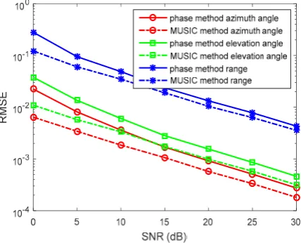
1200, , 6 3

rθ ϕ =_ π π_ in lossless medium system. We determine the SNR from 0 to 30dB, containing N = 1000 snapshots in each run. The RMSEs of the azimuth angles, elevation angles and the range estimations by the phase method are presented in Fig.2. We also determine the N from 500 to 1500 snapshots, containing SNR = 10dB in each run. RMSEs of the azimuth angles, elevation angles and the range estimations by the phase method are presented in Fig.3. The amplitude method and synthesis method are invalid in this situation. MUSIC method is executed to do as the reference.

In the figures, we can see that the accuracy of the phase method is similar to the MUSIC method in the lossless medium situation. For the azimuth angle, elevation angle and range, the phase method can give the accurate results. In the high SNR, the accuracy of the phase method is more close to the MUSIC method. With snapshots increasing, the accuracy of phase method becomes higher.

Fig. 2 RMSEs of location estimations for single-source in the lossless medium versus SNRs.

(

, ,

)

1200, , 6 3

(7)

Fig. 3 RMSEs of location estimations for single-source in the lossless medium versus snapshot.

(

, ,

)

1200, , 6 3

rθ ϕ =_ π π_, the SNR is 10dB & 500 independent trails.

In the second experiment, we set R=300 , f = ×5 10 Hz5 and σ =10−5 . When

12 0 8.8541878 10

ε ε₌ ₌ _× − _{F m}_,₂_{π ε}_f _≈_{2.78 10}_× −5_>_σ _{. The source is located at}

(

_{, ,}

)

_{1200, ,}

6 3

rθ ϕ =_ π π _

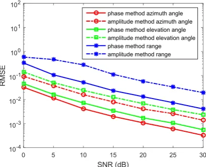
in weak lossy medium system (such as ionosphere). We determine the SNR from 0 to 30dB, containing N = 1000 snapshots. The RMSEs of the azimuth angles, elevation angles and the range estimations by the phase method and amplitude method are presented in Fig.4. We also determine the N from 500 to 1500 snapshots, containing SNR = 10dB in each run. RMSEs of the azimuth angles, elevation angles and the range estimations by the phase method and amplitude method are presented in Fig.5. The synthesis method is invalid because of α β≠ .

In the figures, we can see that the accuracy of the phase method is higher than the amplitude method in the weak lossy medium. With snapshots increasing, the accuracy of phase method and amplitude method becomes higher.

Fig. 4 RMSEs of location estimations for single-source in the weak lossy medium versus SNRs.

(

, ,

)

1200, , 6 3

rθ ϕ =_ π π_, the snapshot number is 1000 & 500 independent trails.

RMS

E

0 5 10 15 20 25 30

SNR (dB)

10-4 10-3 10-2 10-1 100 101 102

RMSE

phase method azimuth angle amplitude method azimuth angle phase method elevation angle amplitude method elevation angle phase method range

(8)

Fig. 5 RMSEs of location estimations for single-source in the weak lossy medium versus snapshot.

(

, ,

)

1200, , 6 3

r_{θ ϕ} =_ π π_

 , the SNR is 10dB & 500 independent trails.

In the third experiment, we set R=30 , f =20Hz and σ =4 . When ε=80ε0 , 3

2π εf _≈2.22 10_× − _<<σ _and _{α β}_{= =} _{π μσ}_f _{. The source is located at}

(

_{, ,}

)

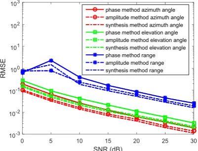
_{120, ,} 6 3

rθ ϕ =_ π π _ in conductive medium system (such as ocean). We determine the SNR from 0 to 30dB, containing N = 1000 snapshots. The RMSEs of the azimuth angles, elevation angles and the range estimations by the phase method, amplitude method and synthesis method are presented in Fig.6. We also determine the N from 500 to 1500 snapshots, containing SNR = 10dB in each run. RMSEs of the azimuth angles, elevation angles and the range estimations by the phase method, amplitude method and synthesis method are presented in Fig.7.

In the figures, we can see that the accuracy of the amplitude method is higher than the phase method in the conductive medium. The synthesis method has the highest accuracy. With snapshots increasing, the accuracy of phase method, amplitude method and synthesis method becomes higher.

Fig. 6 RMSEs of location estimations for single-source in the conductive medium versus SNRs.

(

, ,

)

120, , 6 3

rθ ϕ =_ π π_, the snapshot number is 1000 & 500 independent trails.

0 5 10 15 20 25 30

SNR (dB)

10-3 10-2 10-1 100 101 102 103

RMS

E

(9)

Fig. 7 RMSEs of location estimations for single-source in the conductive medium versus snapshot.

(

, ,

)

120, , 6 3

r_{θ ϕ} =_ π π_

 , the SNR is 10dB & 500 independent trails.

In the fourth experiment, we set R=300, f = ×5 10 Hz5 , N = 1000 snapshots and SNR=10dB. When ε ε= 0, 2π εf ≈2.78 10× −5. The source is located at

(

, ,

)

1200, ,

6 3

rθ ϕ =_ π π_ in lossy medium system. We determine

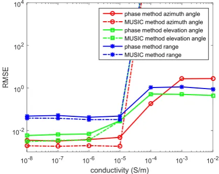
σ

from 10 S m−8 _to_{10 S m}−2 _{. We assume}

σ

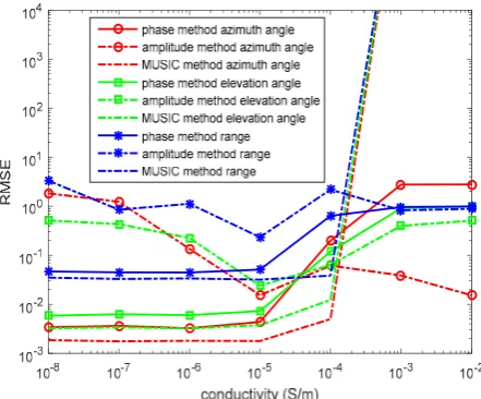
_{is unknown. (the location}

estimations is based on the lossy medium) The RMSEs of the azimuth angles, elevation angles and the range estimations by the phase method and MUSIC method are presented in Fig.8.

In the figure, for the phase method, the location estimations in the low conductive medium is relatively accurate, while the location estimations in the high conductive medium has the low accuracy. The MUSIC method is invalid for estimating the source location in the high conductive medium.

Fig. 8 RMSEs of location estimations for single-source in the lossy medium versus snapshot.

(

, ,

)

1200, , 6 3

rθ ϕ =_ π π_

 ,

σ

is unknown, the SNR is 10dB, the snapshot number is 1000 & 500

independent trails.

In the fifth experiment, we set R=300, f = ×5 10 Hz5 , N = 1000 snapshots and SNR=10dB. When ε ε= 0,

5

2π εf _≈2.78 10_× − _{. The source is located at}

(

_{, ,}

)

_{1200, ,}

6 3

rθ ϕ =_ π π_ in lossy medium system. We determine

σ

from 10 S m−8 _to_{10 S m}−2 _{. We assume}

σ

_{is known. The RMSEs of the}

500 1000 1500

snapshot

10-2 10-1 100 101 102 103

phase method azimuth angle amplitude method azimuth angle synthesis method azimuth angle phase method elevation angle amplitude method elevation angle synthesis method elevation angle phase method range amplitude method range synthesis method range

10-8 10-7 10-6 10-5 10-4 10-3 10-2

conductivity (S/m)

10-2 100 102 104

(10)

azimuth angles, elevation angles and the range estimations by the phase method, amplitude method and MUSIC method are presented in Fig.9.

In the figure, for the phase method, the location estimations in the low conductive medium is relatively accurate, while the location estimations in the high conductive medium have the low accuracy. The MUSIC method is invalid for estimating the source location in the high conductive medium. But the valid range of the MUSIC method with known

σ

is wider than the MUSIC method with unknown

σ

, which we can get from the Fig.8 and Fig.9. The amplitude method has the lower accuracy than phase method in low conductivity, but its results are opposite in the high conductivity.

Fig. 9 RMSEs of location estimations for single-source in the lossy medium versus snapshot.

(

, ,

)

1200, , 6 3

rθ ϕ =_ π π_,

σ

is known, the SNR is 10dB, the snapshot number is 1000 & 500 independent trails.

5. Conclusion

This paper has presented the model and the methods for 3-D single source localization in lossy medium using UCA. And it also analyzes the valid range and computational complexity of the proposed methods and the MUSIC method. We also give the results of methods in lossless medium (air), weak lossy medium (ionosphere) and conductive medium (ocean). In the low conductivity (2π ε σf < ), MUSIC method is valid and the phase method has the higher accuracy than amplitude method. In the low conductivity (2π ε σf > ), MUSIC method is valid and the phase method has the lower accuracy than amplitude method. Of course, in the conductive medium (2π εf >>σ ) the synthesis method has the highest accuracy than phase method and amplitude method.

References

[1] J. H. Lee, D. H. Park, G. T. Park, et al., “Algebraic path following algorithm for localizing 3-D near-field sources in uniform circular array,” Electronics Letters, vol. 39, no. 17, pp. 1283–1285, 2003.

[2] Y. H. Ko, Y. J. Kim, H. I. Yoo, et al., “2-D DoA Estimation with Cell Searching for a Mobile Relay Station with Uniform Circular Array,” IEEE Transaction on Communications, vol. 58, no. 10, pp.2805–2809, 2010. [3] H. Krim, M. Viberg, “Two decades of array signal processing research: The parametric approach,” IEEE Signal

Processing Magazine, vol. 13, no. 4, pp. 67–94, 1996.

[4] R. O. Schmidt, “Multiple emitter location and signal parameter estimation,” IEEE Transactions on Antennas

and Propagation, vol. 34, no. 3, pp. 276–280, 1986.

[5] B. D. Rao, K. V. S. Hari, “Performance analysis of root-MUSIC,” IEEE Transactions on Acoustics Speech & Signal

Processing, vol. 37, no. 12, pp. 1939–1949, 1989.

(11)

theoretical and experimental performance study,” IEEE Transactions on Signal Processing, vol.48, no. 5, pp. 1306–1314, 2000.

[7] R. Rot, T. Kailath, “Esprit-estimation of signal parameters via rotational invariance techniques,” IEEE

Transactions on Acoustics, Speech, and Signal Processing, vol. 37, no. 7, pp. 984–995, 1989.

[8] G. Liu, X. Sun, “Two-Stage Matrix Differencing Algorithm for Mixed Far-Field and Near-Field Sources Classification and Localization,” IEEE Sensors Journal, vol. 14, no. 6, pp. 1957–1965, 2014.

[9] T. Jung, K. Lee, “Closed-Form Algorithm for 3-D Single-Source Localization With Uniform Circular Array,”

IEEE Antennas Wireless Propagation Letters, vol. 13, no. 6, pp. 1096–1099, 2014.

[10] Y. Wu, H. C. So, “Simple and accurate two-dimensional angle estimation for a single source with uniform circular array,” IEEE Antennas Wireless Propag. Lett., vol. 7, pp. 78–80, 2008.

[11] B. Liao, Y. Wu, S. Chan, “A generalized algorithm for fast two dimensional angle estimation of a single source with uniform circular array,” IEEE Antennas Wireless Propagation Letters, vol. 11, pp. 984–986, 2012. [12] Y. Liu, X. Zhang, J. Shao, et al, “Estimation of ship's extremely low frequency electromagnetic signature

based on fuzzy fusion for target detection,” IEEE China Summit & International Conference on Signal and

Information Processing, vol. 158, no. 4, pp. 253–261, 2014.

[13] H. Tao, J. Xin, J. Wang, et al, “Two-dimensional direction estimation for a mixture of noncoherent and coherent signals,” IEEE Transactions on Signal Processing, vol. 63, no. 2, pp. 318–333, 2015.

[14] G. Wang, J. Xin, N. Zheng, et al, “Computationally efficient subspace-based algorithm for two-d imensional direction estimation with L-shaped array,” IEEE Transactions on Signal Processing, vol. 59, no. 7, pp. 3197– 3212, 2011.

[15] B. Xue, G. Fang, and Y. Ji, “Passive localization of mixed far-field and near-field sources using uniform circular array,” Electronics Letters, vol. 52, no. 20, pp. 1690–1692, 2016.

Creative Commons CC BY

, , 1274; doi:10.3390/s17061274