ANALYSIS OF THE TEMPERATURE CHANGES IN
THE ABURRÁ VALLEY BETWEEN 1995 AND 2015
AND MODELING BASED ON URBAN,
METEOROLOGICAL AND ENERGETIC
PARAMETERS.
Enrique Posada1,†,‡and Andrea Cadavid1,‡
1 HATCH INDISA; Carrera 75 No48 A 27 Medellín, Colombia
* Correspondence: [email protected]; Tel.: +57-4-444-6166 Ext:188 † Current address: Affiliation 1
‡ These authors contributed equally to this work.
Version February 5, 2018 submitted to
Abstract: There is a perception among the inhabitants of the Aburrá Valley Region, that this 1
heavily populated region, situated in the Andean mountains of Colombia, has been suffering large 2
temperature elevations in the last years, especially in the last decade. To give perspective about 3
this issue, the authors have gone through the available information about temperature changes in 4
three meteorological stations in the region and have correlated it with a set of variables of urban, 5
climatic and energetic nature, with the intention of developing an approximate model to understand 6
the temperature changes. Changes in the mean temperature, based on the linear correlation of the 7
data were estimated on 0.47oC for the 20 years between 1995 and 2015; the study showed that 60% 8
of change was found to be related to local human activities and 40% was attributed to the impact 9
of global warming. For the local influences some practical mitigation actions are proposed, related 10
to improve the energy management and paying more attention to the temperature changes trough 11
improvements in the number and capability of sampling stations in the urban air and in the river, 12
which serve as clear indicators of the changes and the effect of any mitigation measures. 13
Keywords:Model; Temperature; Urban; Warming. 14
1. Introduction 15
In order to have a better understanding of the temperature behavior of the city of Medellín and its 16
metropolitan area in the Aburrá Valley, situated in the Andean mountains of Colombia, two different 17
urban models are developed, which seek to describe and explain temperature increases and variations 18
in this region in the recent years and how human factors influence this. For the models, the studied 19
time range goes from 1995 to 2015. 20
1.1. Basic model description and objectives 21
Although the models here developed are simplifications of reality, building them is a somewhat 22
complex procedure, considering the type of variables that influence temperature changes and the fact 23
that a populated valley is subjected to climate, topographic, energy and activity factors. To facilitate 24
the understanding and logical following of the steps considered in the models, flow diagrams have 25
been prepared and presented in figuresA1andA2in the AppendixA. The model considers two 26
descriptions of the temperature changes. One of them is the tendency of the change, described by 27
means of the linear correlations of temperature data with time; the other one considers the variations 28
of the temperatures in reference to the linear tendencies. For the prediction of the linear tendency, 29
two models are applied: one based in an energy balance that considers the region as a control volume 30
with energy inputs and outputs; and another one based on factors related to human interactions and 31
activities. For both models, the goal is to have an approximation to the relative importance of the 32
factors influencing the linear tendencies, but first it is required to understand in which grade they 33
depend on local factors or on external (global ones, such as global warming). So, a methodology was 34
developed to isolate these two major influences. Once the local effects are determined, the goal is to 35
propose some mitigation actions, resulting from the relative importance of the causing factors. For 36
the case of the variations of the temperatures with relation to the linear tendencies, correlations were 37
developed based on local variations of sunshine duration and precipitation and on globalLa Niñaand 38
El Niñophenomena. The goal was to get an approximation and understanding of those ups and downs 39
in the temperature change, which difficult the interpretations of temperature data on the short term. 40
Another objective is to contribute to a more objective community perception of the climate change 41
in the region, as there is the common perception of the citizens that the inhabited zone of the Aburrá 42
Valley is notably increasing its temperature [1] [2]. A simple survey of 50 people from the engineering 43
company where the authors work, gives an indication of this perception. They believe that in the last 44
five years the temperature has increased by 1.8±1.3oC and that the average temperature of Medellín 45
corresponds to 23.6±2.8oC. While this shows a good approximation to the average temperature, 46
the increase perceived is grossly exaggerated compared to the reality, as our study shows. It seems 47
that with news continuously mentioning global warming and how the temperatures of the planet are 48
increasing [3], this influences perceptions in the direction the survey indicates. The authors consider 49
that it is important to study these phenomena with an objective view, to really understand what the 50
heating impact of the urban activities on the zone is, as compared to the impact of global warming; 51
and to find which agents could cause the changes. In this way, citizens can better understand the 52
situation and act in some way to assume the changes and mitigate them. This study is a first step in 53
the direction of examining possible solutions at least at the local level. However, it is believed that the 54
same concepts can be applied elsewhere. 55
1.2. Urban temperature changes. Literature and state of the art review. 56
Several scholars around the world have undertaken the task of understanding, studying, 57
quantifying and seeking alternatives to mitigate temperature changes in urban areas and their areas of 58
influence. There are several types of models that have been developed and presented as tools, and they 59
have a certain similarity with the models presented in this paper. In general, these studies contribute 60
to clarify the variables that are taken into account and their importance in the climate of urban areas 61
around the world. In them it is noticed the global interest and the actuality of this type of studies. 62
Several authors seek to characterize urban climate change; Xu et al [4] analyzed five long-term 63
meteorological parameters to characterize climate change in the city of Urumqi, China. Huang and 64
Lu [5] do something similar for the urban agglomeration of the Yangtze River delta, also in China, 65
where with the use of the maximum, average and minimum temperature observations, a heating rate is 66
determined and compared to the averages, also correlations with factors such as speed of urbanization, 67
population and built area are done. Fujibe [6] analyzes data for 561 stations for 27 years in Japan, 68
where the contribution of urban effects to temperature trends are studied, classifying the stations by 69
the population density around them. 70
Another field is the Urban Heat Islands, (UHI) studies. For example, Grimmond [7] seeks 71
to estimate the local effect of cities on climate, as well as their causes, dynamics and mitigation 72
strategies, Lauwaet et al [8] estimate the heat island in Brussels and project it to 2060- 2069, by relating 73
meteorological parameters with the UHI. Fuentes [9] does the same for Tampico, Mexico, characterizing 74
the urban zone and studying the historical macro climate to determine the urban heat island. Stone 75
[10] makes an analysis for 50 metropolitan areas in the United States and establishes the warming per 76
decade for urban and rural areas and heat island intensity for 50 years. In works like Djedjig et al [11], 77
urban climatology; the first two study the mitigation of the heat island effect through the use of green 79
roofs and walls and the latter determines the heating potential of three different land uses. 80
Most of the reviewed models are based on energy balances, these study the energy flows of the 81
city or account the energy inputs as well as its consumption characteristics. In the work of Kiss [14] a 82
model of the city of Pécs, Hungary, is presented, which takes into account the energy from heating, 83
electricity and transport. The study by Chow et al [15] estimates the heat emissions of anthropogenic 84
nature, with inventories of population density, traffic and electricity consumption for the city of 85
Phoenix, United States. Song et al [16] propose a mass and energy balance model, which evaluates 86
the efficiency of 31 Chinese cities and determine their sustainability; inputs and outputs such as 87
energy, materials, investment capital, waste, production and others are considered. In the city of 88
Kiruna, Sweden, Johansson et al [17], analyzed the energy model to see the possibility of achieving the 89
performance goals imposed by the national government. 90
At the national level there are models of determination of energy flows for the city of Pasto by 91
Gómez et al [18], they present it as a tool for the planning of a sustainable city. For the city of Bogotá 92
there is the work of Diaz [19],[20],[21] in which he seeks to understand the urban metabolism, with the 93
quantification of inputs and outputs of energy, food, fuels, among others, versus their methodologies 94
of supply, transformation, consumption and disposal to determine their impact and diagnose the 95
sustainability of the metropolis. No studies on temperature change related to global warming or 96
local activities were found applicable to the Aburrá Valley, nor there are studies that use the specific 97
modeling strategies proposed here. The authors feel that their contribution is a valuable one. 98
1.3. Basic information about the studied region. 99
The region to be studied is the Metropolitan Area of the Valley of Aburrá (AMVA by its acronym 100
in Spanish) that is made up by the municipalities of Caldas, Itagüí, Sabaneta, Bello, Copacabana, 101
Girardota, Barbosa, La Estrella, Envigado and Medellín (which is the major city, with 65% of the 102
population). This is the second largest metropolitan area of Colombia, after the metropolitan area of 103
Bogotá, the capital city. In total it has approximately 3.8 million inhabitants and urban and rural areas 104
of 102 km2and 1054 km2respectively. It is located in the center of the department of Antioquia, on 105
the central chain of the Andes mountain range with an average elevation of 1538 m. Located on the 106
tropic, it has quite constant temperatures and small climate variations throughout the year. The area is 107
located in a valley formed by two mountain ranges one to the east and the other one to the west and is 108
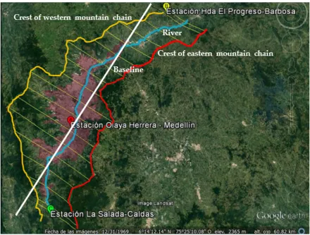
crossed by the Medellín river, as shown in Figure1 109
In the Figure1, three irregular lines are observed, two representing the crests of the mountain 110
ranges on each side of the valley, and a third one, the river that runs through the middle of the valley. 111
A fourth and straight line is a reference, called “baseline”, which is formed by joining a point in the 112
south west with coordinates 6o02’18.51 " North 75o41’38.70" West with a point in the north east with 113
coordinates 6o28 ’ 47.19 " North 75o24’58.90" West. This line serves as the axis for the location of 114
distances from the southern to the northern extremes of the valley, and following the direction of the 115
flow of the river. The figure also shows clear demarcated reddish shade urban areas. The position 116
of the three measuring stations is also displayed. These correspond to meteorological measurement 117
points and are the only stations in the region that have the historical data necessary for the study to be 118
performed. The station Hacienda el Progreso is located in Barbosa, which is an area rural in nature 119
and is the place where the winds enter the valley. The station at the Olaya Herrera Airport, located in 120
the center of the valley, corresponds to an urban area and finally the station La Salada in Caldas, is a 121
more rural area and at a higher elevation than the previous two, so it is cooler; here the wind leaves 122
Figure 1.. Location of the studied region with river line, baseline and distances between crests of the valley, perpendicular to baseline. c2015 Google Inc.
2. Data basis and Methods 124
The starting point is the collection of data from different sources of information for the diverse sets 125
of variables. These have to do with the climate (local and global), the geography, the river temperatures, 126
the demographic, economic and activity variables and indicators. 127
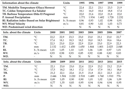
2.1. Information about the climate 128
Table1shows the mean measured values of temperature in the different stations of the Valley 129
and the precipitation, radiation, wind velocity and predominant wind direction in the Olaya Herrera 130
Airport station. The variables in this group are thought to have influence or are associated with the 131
temperatures of the city. 132
The main variable to be studied, temperature, is collected from IDEAM, a reliable data source, 133
"a public institution of technical and scientific support to the National Environmental System, which 134
generates knowledge, produces reliable, consistent and timely information, on the state and dynamics 135
of natural resources and the environment" [22]. This is the national office responsible of scientific data 136
on climate. Historical data was obtained for the three stations mentioned above. The model considers 137
the average annual temperature. Figure2shows the evolution over time for the three measuring 138
stations and their linear adjustment. The shown linear correlations allow observing tendencies and 139
trends. 140
As shown in Figure2, mean temperatures vary from year to year, with variable behaviors that 141
cannot be easily explained. In any case it is observed that there are trends. In the case of Medellín 142
with a very small increase. These observations allow to assert that the causes for the warming in 144
Medellín and Caldas have to do with the human activities in the urban area of the Valley of Aburrá, 145
since these stations somehow have urban nature and receive the influences of the urban activities, 146
stimulated by the predominant direction of the wind, from north to south, from Barbosa to Caldas. In 147
contrast the Barbosa station does not receive this type of influences. But all of this has to be looked at 148
within the context of geographic variables, especially altitude above sea level of the station, since in 149
the mountainous tropical region temperatures tend to change with elevation. 150
Table 1.Values of the different climatic variables to be considered in the study.
Information about the climate Units 1995 1996 1997 1998 1999
TM. Medellín Temperature (Olaya Herrera) oC 22,4 22,1 23,1 23,3 21,9
TC. Caldas Temperature (La Salada) oC 18,1 16,0 18,4 18,8 17,4 TB. Barbosa Temperature (Hda El Progreso) oC 22,0 21,6 22,0 21,8 22,0
P. Annual Precipitation mm 1.771 1.934 1.402 1.728 2.232
RI. Radiation index (based on Solar Brightness) h /h mean 0,96 0,93 1,02 0,98 0,91
WV. Wind Velocity m/s 0,81 0,90 1,02 1,03 0,73
WD. Predominant wind direction - N N N N N
Info. about the climate Units 2000 2001 2002 2003 2004 2005 2006 2007
TM. oC 22,2 22,9 23,3 23,0 23,0 23,1 23,0 22,7
TC. oC 17,4 18,1 18,3 18,2 18,0 18,5 18,6 18,6
TB. oC 22,3 23,0 22,8 22,9 22,8 23,0 22,9 22,3
P. mm 2.132 1.412 1.450 1.650 1.844 1.801 2.025 2.048
RI. h /h mean 1,01 1,05 1,10 1,03 1,06 1,00 0,97 1,01
WV. m/s 0,93 0,98 0,93 0,85 0,92 0,88 0,82 0,83
WD. - N N N N N N N N
Info. about the climate Units 2008 2009 2010 2011 2012 2013 2014 2015
TM. oC 22,1 23,0 23,0 22,4 22,9 23,2 23,2 23,9
TC. oC 17,5 18,2 18,1 17,2 17,6 17,9 18,1 18,6
TB. oC 21,2 22,1 22,6 21,5 21,8 22,1 22,3 22,7
P. mm 2.446 1.504 2.220 2.518 1.489 1.740 1.910 776
RI. h /h mean 0,89 1,05 0,90 0,90 1,01 1,02 1,06 1,09
WV. m/s 0,77 1,35 0,83 0,95 0,94 0,94 0,94 0,95
WD. - N N N N N N N N
2.1.1. Temperatures 151
Figure2shows the average annual temperatures for the three stations: Barbosa (Hda el Progreso), 152
Medellín (Olaya Herrera) and Caldas (La Salada), and their respective linear trends between 1995 and 153
2015. The Medellín station, corresponding to the central zone of the Medellín city, shows the correlation 154
with a higher increase tendency. The Barbosa station, which is situated in a rural area, upwind from 155
the urban areas, shows a very stable tendency, with very small change. The Caldas station, which 156
is situated in an area of mixed rural and urban background and downwind from the main urban 157
Figure 2.Average annual temperatures for Barbosa (Hda el Progreso), Medellín (Olaya Herrera) and Caldas (La Salada) stations and their respective 20 year averages and linear correlations between 1995 and 2015.
2.1.2. Annual precipitation 159
The rains were characterized based on the annual precipitation at the Olaya Herrera Airport 160
station; data is obtained from the IDEAM database. This variable is relevant because it is related to 161
local variations in the temperatures, among others, because of the energy exchanges associated with 162
the evaporation of rainwater. Figure3shows the behavior in the study period, significant annual 163
variations are observed, with a relatively stable average trend during the 20 years, around 1810 mm, 164
with a very slight increase in time. 165
Figure 3.Annual precipitation in the studied years
2.1.3. Sunshine duration 166
This variable is measured by the IDEAM at the Olaya Herrera station, as the daily hours of solar 167
the average of the study time, which for the period of available measurements (since 1998), was 4.94 169
hours daily. The result of the ratio between the average value of each year and this average of all 170
measurements has been taken as an indicator of solar brightness, which is related to solar incident 171
radiation in the region. In Table1the values between 1995 and 1998 were estimated based on a 172
correlation between average temperature and sunshine duration. This variable was taken as indicating 173
solar radiation effects. Figure4shows the behavior. 174
Figure 4.Radiation index in the metropolitan area for the studied years.
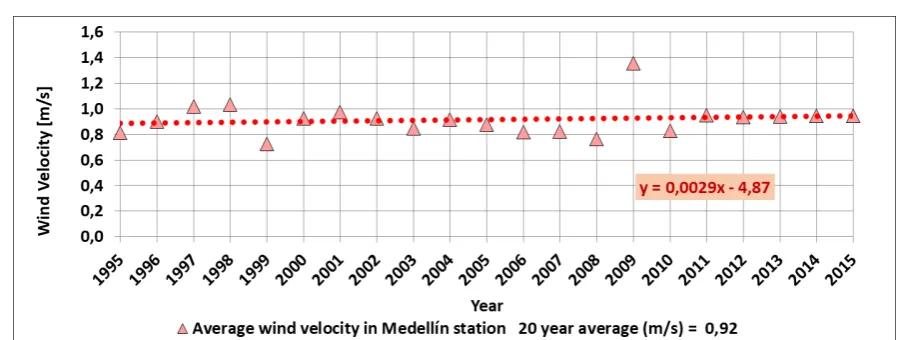
2.1.4. Wind Velocity 175
The average wind velocity data for each of the study years was used and obtained for the Olaya 176
Herrera Airport station from IDEAM. Relatively constant annual mean values were observed in the 177
study period, on which the mean value was 0.92 m/s. In 2009 there is an unusual peak of 1.35 m/s. 178
Figure 5.Average annual wind velocities.
2.2. Geographical information 179
Different geographic features have been considered in the study because of their influence on the 180
climate, like elevation above sea level and also their association with urban activities. Likewise, the 181
temperatures and the flow of the river have been taken into account. The river acts as an important 182
sink of heat taking heat losses from activities in the region. This is evident from its temperature, which 183
2.2.1. Elevation of the topographic levels of the valley 185
The elevation above sea level has an effect on the climate in tropical mountain regions. The 186
following figure shows the geographical situation in the Aburrá Valley, showing the height of the 187
mountain ranges to the east and west of the valley and the height of the river. The graph has taken 188
as a reference the straight line shown in Figure1, called baseline. The elevations of the points of the 189
three considered topography lines were taken at points joined perpendicularly from each line to the 190
baseline. It is observed that the river descends 552 meters in the 51 kilometer length of the baseline, 191
going from 1,862 m to 1,301 m, with an average height of 1,505 m as it passes through the valley. The 192
two mountain ranges have maximum heights of around 3,000 m. The average elevation of the eastern 193
mountain range is 2,584 m and for the western one is 2,529 m. The average elevation in relation to the 194
river is 1,078 m and 1,024 for the eastern and western ranges respectively. 195
Figure 6.Elevation profile for the Aburrá Valley mountain chains and river.
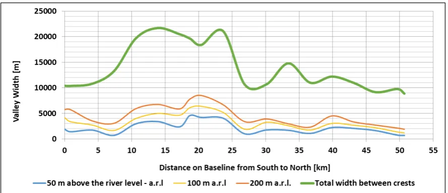
2.2.2. Width of the Valley 196
An analysis of the width of the valley was made at different elevations, 50, 100 and 200 meters 197
above the level of the river, as well as in the ridges of the mountain ranges that form the valley. This 198
was done for different points following the already described reference line that connects two reference 199
points of the valley from south to north. It can be seen in Figure7that the valley it is relatively enclosed, 200
with total areas of 108 km2in the flat zone near the river with less than 50 m above the level of the 201
same, of 166 km2in the zone of less than 100 m above the level of the River, of 227 km2for the zones of 202
less than 200 m above the level of the river and of 718 km2between the ridges of the two mountain 203
ranges that form the valley. The fact that the valley is a box-like system allows it to be seen as a control 204
volume from the point of view of mass and energy flows, in which mountains act as clear boundaries 205
through which energy and air do not flow significantly. On the other hand, the southern and northern 206
ends are inlets and outflows, especially if is taken into account that the winds have predominant 207
directions from the north, following the direction opposite to the flow of the river. 208
2.2.3. River temperature and flow 209
There is evidence that the temperature of a water current, under equilibrium conditions, is related 210
to the ambient air temperature, with a behavior that adjusts to a linear trend [23]. In the case of a river 211
contaminated with hot discharges, it is expected that the current temperatures will move away from 212
the equilibrium curves originated in the ambient air temperatures, with temperature differences (delta 213
T) being related to the levels of thermal contamination. 214
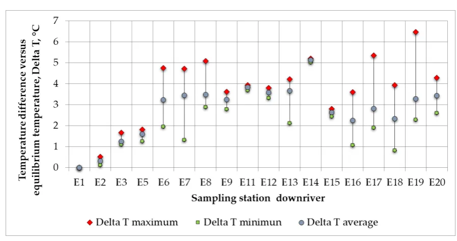
Figure 8.Temperature difference versus equilibrium for the river in each of the measuring stations E1 to E20. Figure taken and adapted from [24].
In that way, it has been considered that the river acts as a sink that evacuates part of the 215
heat generated by the energy systems of the region. This means that the river suffers increases 216
in temperature, additional to the ones expected from equilibrium conditions downriver (which depend 217
on atmospheric pressure). An existing study for the Medellín River [24] is used, which presents these 218
increases in river temperature in zones with urban impact for the year 2006,corresponding to the 219
stretch between stations E2 (called Primavera Station at the south of the valley) and E14 (called the 220
Parque de las Aguas station at the north of the valley, where the Medellín River receives a high flow 221
of water coming from the diversion of the Rio Grande, which causes the cooling of the waters and 222
a new temperature pattern). The temperature difference was on average,4.5oC, as shown in Figure 223
which was 546.4 MW. This magnitude was compared for that year with all the energy coming from 225
the anthropogenic activities and a factor was found that relates the sink to the total of the energetic 226
contributions. This factor was applied to the other considered years since there was no information 227
for river temperatures in the other years of the study. The authors acknowledge that although this 228
is methodologically correct, it is a limitation in the analysis as compared to the fact that for all other 229
considered variables real annual information has been used. On the other hand, it is proposed that the 230
river temperature profile may be used as a real time indicator of city island factor behavior. For this, a 231
temperature measuring system should be put into place. 232
To elaborate the heat flow calculations for the model, it is estimated that, on average, the Medellín 233
River has a medium flow at the entrance to the AMVA of 1.0 m3/s and that after passing through the 234
urban area it has 30 m3/s; this means a medium increase in flow of 29 m3/s. 235
2.3. Information on demographic and economic variables 236
Table 2.Values for the demographic and economic variables considered, every five years.
Variables Units 1995 2000 2005 2010 2015
Living beings
Men millions 0,917 1,023 1,122 1,214 1,299
Women millions 1,096 1,223 1,341 1,451 1,553
Children millions 0,662 0,739 0,810 0,877 0,938
Rodents (rats y mice) millions 36,4 40,8 44,7 47,9 50,5
Cats millions 0,132 0,147 0,161 0,175 0,187
Dogs millions 0,667 0,744 0,816 0,883 0,945
Total equivalent men millions 2,432 2,713 2,975 3,217 3,440
Food and residues
Food consumption million tons/ year 1,01 1,14 1,28 1,41 1,53 Urban Solid Waste generation million tons/ year 0,65 0,73 0,80 0,88 0,96 Economy – annual data
Urban constructed area km2 76,4 83,3 85,4 87,3 88,6
Gross Domestic Product GDP Billon (COP, $) 18,5 21,1 26,0 33,0 42,7 Vehicle fleet
Automobiles thousands 168 209 290 412 575
Motorcycles thousands 50 69 203 437 718
Buses thousands 7,1 8,7 11,4 16,1 22,8
Trucks thousands 12,0 17,0 18,7 26,5 34,3
Taxis thousands 3,6 8,8 20,0 45,3 78,5
Equivalent Vehicles thousands 549 741 1.001 1.549 2.229
Fuels and energy – annual consumption
Gasoline million gallons 124,4 154,8 141,0 140,7 185,9
Diesel million gallons 65,9 82,0 100,5 109,6 148,0
CNG for Vehicles million m3 0,0 1,4 27,2 50,9 65,6
Natural Gas million m3 178 193 218 295 372
Coal million tons 0,319 0,249 0,199 0,188 0,161
Electricity TWh 4,62 4,65 5,37 6,18 7,26
Total Energy million Equivalent
gasoline gallons 438 482 518 578 723
For the modeling, the influence of energy use and human activity has been considered. 237
Demographic variables have been considered, as well as those related to the economic activity of the 238
region. Two models have been developed, one which includes the direct impact of energy variables 239
consuming activities. In the second analysis a change factor was determined to visualize the variables 241
as homogeneous, dimensionless sets. Indexes have been created that correspond to the relation 242
between the real values for each given year divided by the value of the first year of the study and 243
which quantify the relative growth of each variable. Table2shows the data every five years. The model 244
worked with information for each year. In several cases, such as the information on living beings, 245
vehicles and energy, values were processed to obtained equivalent men, equivalent vehicles and 246
equivalent gasoline, respectively, to simplify the modeling. The data used was collected from different 247
public institutions repositories like Banco de la República [25], DANE [26], Alcaldía de Medellín[27] 248
[28] and UPME [29]. 249
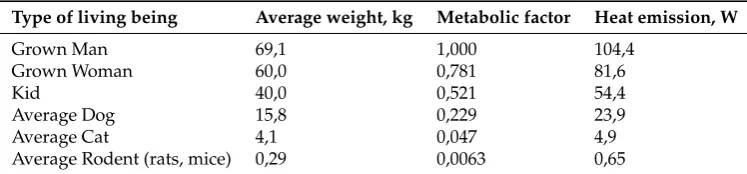
2.3.1. Equivalent Men (Living Beings) 250
The living beings that inhabit the region contribute with their metabolisms to change the 251
temperature of the environment. It has been considered that not only people are contributing in 252
this instance, but also other living beings in a close relationship with humans such as pets and 253
domestic rodents (rats and mice). The equivalent men concept seeks to consolidate the number of men, 254
women, children, pets and rodents in the AMVA region [30] [31]. The equivalence was calculated in 255
accordance to the mean body mass of each type of living being and compared with respect to an adult 256
male weighing 69.1 kg [32]. 257
Table 3.Heat contribution by type of living being.
Type of living being Average weight, kg Metabolic factor Heat emission, W
Grown Man 69,1 1,000 104,4
Grown Woman 60,0 0,781 81,6
Kid 40,0 0,521 54,4
Average Dog 15,8 0,229 23,9
Average Cat 4,1 0,047 4,9
Average Rodent (rats, mice) 0,29 0,0063 0,65
2.3.2. Food 258
This indicator estimates the amount of food consumed by the AMVA inhabitants per year, but it 259
is limited only to humans, the feeding of pets and other living beings is not considered. For calculating 260
this indicator the change over time in food intake per person [33] and the population are considered 261
[34]. 262
2.3.3. Urban Solid Waste 263
It is considered that the amount of waste generated by the population has influence on the heating 264
of the city, since it is an indicator of the consumption habits of a society and its sustainability. The 265
data is taken from a projection made by the AMVA for the formulation of the integrated regional solid 266
waste management plan [35]. 267
2.3.4. Constructed Urban Area 268
The built area of the city is estimated; here a known value reported in a given year is taken 269
into account, starting from this value and an annual indicator of the new constructed area, the total 270
constructed area is estimated [25]. This indicator is important since the built areas have a negative 271
impact on the temperature change (causing it to raise) unlike the green areas and parks; these green 272
areas absorb CO2and heat, so that as the urban area increases, this ecosystem regulation service is 273
2.3.5. Gross Domestic Product – GDP 275
This is an indicator of the total goods and services produced by AMVA annually; it is a 276
representative value of the production and services activity of the city [25]. 277
2.3.6. Equivalent vehicles 278
To calculate this indicator, equivalence factors are found between a light vehicle (automobile) 279
and the other considered vehicles. These equivalences have been estimated based on specific average 280
consumption and daily activity time, for each type compared to a normal automobile. Table4shows 281
the used equivalence factors. 282
Table 4.Equivalence factors between vehicles.
Type of Vehicle Consumption, km/gal urban
Functioning hours
in the day Equivalence factor
Automobiles 30 2 1.00
Motorcycles 100 2 0.30
Buses 8 10 18.75
Trucks 5 6 18.00
Taxis 30 10 5.00
2.3.7. Fuel consumption in terms of equivalent million gallons of gasoline 283
This is an indicator of the city’s energy consumption, since fossil fuels and electricity are counted 284
here. The equivalence is done in relation to the calorific power of each energy source. This indicator 285
can better quantify the influence of transport and energy consumption, because even though the 286
number of vehicles increases, technologies evolve and have better fuel yields, each time requiring less 287
energy per unit distance. The consumption data was obtained from different Statistical Bulletins of 288
Mines and Energy done by UPME (Colombian Energy and Mining Planning Unit) [29]. 289
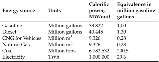
Table 5.Calorific power of the sources and equivalence factor with gasoline gallons.
Energy source Units
Calorific power, MW/unit
Equivalence in million gasoline gallons
Gasoline Million gallons 33.822 1,00 Diesel Million gallons 40.445 1,20 CNG for Vehicles Million m3 9.326 0,28
Natural Gas Million m3 9.326 0,28
Coal Million tons 6.782.532 200,5
Electricity TWh 1.000.000 29,6
Based on the variables that have been described, a model for the annual behavior of the 290
temperature has been developed, which includes the direct impact of energy variables and the indirect 291
impact of demographic and economic variables. 292
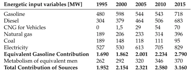
2.4. Information on energetic variables 293
A second model has been developed from a purely energetic point of view, based on energy 294
Table 6.Energy contributions from different sources. Data every five years in MW.
Energetic input variables [MW] 1995 2000 2005 2010 2015
Gasoline 480 598 544 543 718
Diesel 304 379 464 506 683
CNG for Vehicles 0 1,5 29 54 70
Natural gas 189 206 233 314 396
Coal 189 148 118 111 95
Electricity 527 530 613 705 829
Equivalent Gasoline Contribution 1.690 1.862 2.001 2.234 2.790 Metabolism of equivalent men 262 292 320 346 370 Total Contribution of Sources 1.952 2.154 2.321 2.580 3.160
According to the previous table, the region receives a total energy contribution that currently 296
exceeds 3 000 MW. This contribution essentially dissipates into the medium, even if it is useful energy, 297
since eventually it will generate heat, friction, noise and other dissipative forms. 298
2.5. Dimensional adjustment and treatment of variables 299
2.5.1. Transformation of temperatures 300
As shown in Figure2, temperatures at the different points in the metropolitan area have different 301
behaviors. For the case of Barbosa (Hda. El Progreso), the temperature shows relatively moderate 302
variations in the 20 years of the study. In the case of Medellín (Olaya Herrera) and Caldas (La Salada) 303
a variable but gradual warming is observed, being more prominent in Medellín. This warming is 304
considered a result of the regional anthropogenic reasons treated in this model. However, it is clear 305
that there are other causes that must be taken into account. 306
On the one hand there are the impacts of phenomena of a global nature, which in principle are 307
distributed all around the planet, with certain geographic variations. Figure9shows the data provided 308
by the NOAA’s National Climatic Data Center [36], with global temperatures of the surface of the 309
earth, compared against the average between 1901 to 2000 (dotted line passing through zero). The 310
impacts of the Niño (increases) and the Niña (decreases) phenomena are observed. Niña and Niño 311
are names customarily used for these warming and cooling periods. From 1995 to 2015, on average, 312
an increase is not observed, but rather some decrease is noted. Figure10shows the behavior of such 313
global temperatures compared to those of the studied region in the Aburrá Valley. For this purpose, 314
the data has been processed in the following way: 315
• After converting the global delta temperature fromoF tooC, the information was digitized to 316
semester and annual values, from which the data of 1995, the first year contemplated in our 317
study, were subtracted. Thus, DTGS 95 annual and DTGS 95 semester (semi-annual) curves were 318
obtained. 319
• The three annual temperatures of the region, Barbosa (TB, Hda. Progreso), Medellín (TM, Olaya 320
Herrera) and Caldas (TC, La Salada) were taken and their average values in 1995 were subtracted 321
of each, thus obtaining the TM-TM95, TC-TC95 and TB-TB95 curves. 322
Figure10clearly suggests that the impacts of the Niño and Niña phenomena (associated with 323
up and down changes) are related to the temperature oscillations for the three stations in the region. 324
Such oscillations follow quite well those of global temperatures. However, trends, as seen in linear 325
adjustments, differ from global phenomena to local phenomena. This is to probably related to the local 326
behavior of air masses in a relatively long, narrow and enclosed valley between two mountain ranges 327
with 1000 m height, valley in which the urban activity of nearly four million people has a significant 328
Figure 9.Global annual temperatures of the earth surface (oF), compared against the average 1901 to 2000 (dotted line passing through zero), data from NOAA’s National Climatic Data Center. The impacts of the Niño (increases) and the Niña (decreases) phenomena are observed [36].
Figure 10.Comparison between the annual global temperatures of the surface of the earth and the temperatures of the stations of the Aburrá Valley (Deltas against 1995).
Because the anthropogenic factors tend to grow continuously with time without major oscillations, 330
correlation with time (Figure2). The differences between the actual temperatures and the linear 332
correlation, then, are caused by non-anthropogenic nature effects. Figure11shows the actual Medellín 333
station (TM) temperatures, their linear correlation (TMTA, TM temporal adjustment) and the deltas 334
DTTM (defined as DTTM = TM –TM temporal adjustment). 335
It was postulated that such deltas (DTTM) depend on phenomena that are not anthropogenic. For 336
this case, these non-anthropogenic phenomena are, on the regional scale, the local climate influences, 337
taken here as the other major variables besides temperature: average annual rainfall and average 338
annual radiations and, on the global scale, the universal phenomena of the Niño and Niña, as noted in 339
Figure9and Figure10. 340
• Global Niño and Niña factor.DTGS (global DTGS vs. average global DTGS), taken from Figure9 341
and Figure10. 342
• Radiation excess factor (radiation index - minimum radiation index). The radiation index has 343
been defined as the annual sunshine hours divided by the average annual sunshine hours in the 344
studied period. This average value was 1,800 hours per year. The factor is calculated by subtracting 345
from the annual index the minimum registered index (0.86), which occurred in the year 2008 with 346
a total of 1,599 hours. 347
• Precipitation defect factor (maximum precipitation index - precipitation index). The 348
precipitation index has been defined as the annual precipitation value in mm of water, divided by 349
the average annual precipitation in the period studied. This average value was 1,811 mm per year. 350
The factor is calculated subtracting the maximum recorded index (1.39), which occurred for the 351
year 2011 with a total of 2,518 mm, from each of the annual indices. 352
Figure 12.Temperatures deltas for Medellín and global and climate factors between 1995 and 2015.
Figure12show the behaviors of DTTM and the said indicators of radiation, precipitation and 353
global phenomenon. Figure12clearly suggest that the impacts of the Niño and Niña phenomena, 354
the Radiation factor and the Precipitation factor and their up and down changes are related to the 355
temperature oscillations. Table7shows the obtained correlations that can be considered as significant 356
as they have high correlation factor. They are therefore used to predict annual temperature behaviors 357
with relation to DTTM variations against the annual linear adjustment. 358
Table 7. Correlations found between the temperature delta and the global temperature change, radiation and precipitation.
Influence and factors R2
FIDT global = global, Niño and Niña Factor (DT global vs mean) 0,400
FIR = Radiation Factor 0,520
FIP = Precipitation Factor 0,626
To better understand the changes over time already presented in Figure2, temperatures for 359
stations M and B between 1990 and 2015 are shown in Figure13. This shows more clearly that the 360
changes in Medellín are greater than the time changes in Barbosa. A first important consideration 361
was to assume that the change in temperatures in Barbosa corresponds to impacts attributable to 362
the mixture of global and local climatic impacts and not to impacts of the activity of the region, this 363
taking into account the situation of such a station in the rural north of the valley, and the predominant 364
direction of the winds, which go from north to south. These two facts indicate that the Barbosa station 365
Figure 13.Average annual temperatures in the stations of Barbosa and Medellín between 1990 and 2015 and their linear adjustments over time.
A second consideration is to assume that the difference between the temporary temperature 367
adjustments of Medellín (TM) and Barbosa (TB) is due to human activity in the region. This activity 368
generates: 369
• Continuous and increasing heat emissions, which origin increases in the temperature of the air 370
passing through the urban area. 371
• Changes in patterns of heat exchange and absorption and emission of solar radiation. For example, 372
increases in the constructed area and in the corresponding circulation surfaces, ceilings and walls 373
result in changes in surface emissivities and changes in absorptances and reflectances. 374
• Secondary reactions involving the presence of atmospheric agents and pollutants, which supply 375
and consume reaction energies and change in the parameters of absorption and emission of 376
radiation. 377
A value of 0,06oC (DTSNM) has been discounted from the linear adjustment of temperatures in 378
Medellín (TMAT) and Barbosa (TBAT), considering that station M is at 1,490 m above sea level and 379
the station B is at a slightly higher elevation, 1,500 meters above sea level. In this way, based on time, 380
the temperature difference due to the activity has been constructed as indicated by (1). This DTAM 381
difference is the one to be modeled. 382
DTAM=TMAT−TBAT−DTSNM (1)
2.5.2. Indexing of Activity Indicator Variables 383
As already mentioned, indices have been created for the different variables, which correspond to 384
the relation between the real value for each year divided by the value for the first year of the study 385
(1995). These indices also quantify the relative growth of each variable. 386
2.6. Correlations Establishment 387
Two models of linear nature are made to approximate the modeling of temperature increases 388
as a function of the considered anthropogenic activity factors. The first one based on the factors of 389
human activity and the second one based on inputs and outputs of energy to the mixture zone of the 390
The first model assumes that the DTAM temperature changes are the result of a linear combination 392
of the indexes of the activity indicator variables. 393
DTAM(modeled) =
∑
FAi∗IAi (2)WhereFAiis the activity influence factor andI Aiis the annual activity index for the variablei. 394
To find the influence factors for each variable an Excel Solver routine was used and executed 10 395
times minimizing in each occasion the average of the absolute values of the annual error (this error was 396
obtained comparing real DTAM against modeled DTAM), changing the initial values of the assumed 397
factors in the interaction, so that different results are obtained each time. At the end the obtained 398
factors are averaged. 399
It is important to understand that this is not a closed problem and that there are multiple 400
combinations that approach the real value of DTAM. There is a high number of parameters in 401
comparison to only 20 years. Because of this, there is no pretense to demonstrate the validity of 402
the obtained linear regression, except inasmuch as the model fits the observation reasonably well 403
permitting a useful approximation to the influence of the studied activity factors, which can be used to 404
propose recommendations such as the ones expounded in this work. 405
The second model is based on an energy balance in which the energy inputs described in Table6 406
are considered. The heating that the Medellín River suffers due to the activity while passing through 407
the region has been considered in the model as an energy output. A control area has been considered, 408
the width of this area corresponds to an average between the medium width of the valley at 50 m 409
above the river level from Barbosa to Medellín stations and the width between the mountain ranges 410
at the mixing height; the height of the control volume was chosen such that it gives a good fit of the 411
model. Table8shows the values for these variables. The energy balance is described by the following 412
expression: 413
Qin−Qout=mair˙ ∗Cp∗∆T (3)
Where: 414
Qin: Annual energy Input to the Control Volume. Comes from the energy sources.
415
Qout: Thermal energy output that leaves the control volume through the river.
416 ˙
mair: Air Mass flow that goes through the control volume.
417
Cp: Specific heat of Air.
418
∆T: Air temperature change suffered by the air traveling between the ends of the control volume. 419
420
For the annual energy input, a percentage of the total energy of the entire Aburrá Valley was 421
considered, taking into account that the temperature change occurs up to the Olaya Herrera station. 422
This percentage is proportional to the distance in the central axis from the north to the Olaya Herrera 423
station, compared to the total distance between the two ends, Caldas and Barbosa, obtaining a 424
percentage of 60.17%; this considers the preferential direction of the wind, from north to south. As for 425
the output of energy carried by the river, a 39.43% of the same (100 - 60.17)% is considered since the 426
River drags energy in the opposite direction to the wind, from south to north. In order to estimate the 427
annual average mass flow, the average wind speed in the mixing zone which was estimated at 2.64 428
times the velocity at the surface, was multiplied, by the control area and by the air density, for each 429
Table 8.Dimensions of control volume associated with energy balances.
Average elevation of the Mountain ranges from North
to Olaya Herrera in relation to the river elevation m 1.086 Average width from North to Olaya Herrera at 50 m
height above the River, flat area m 1.923
Average width from North to Olaya Herrera at 100 m
height above the River m 2.870
Average width from North to Olaya Herrera at 200 m
height above the River m 3.846
Average width from North to Olaya Herrera at mixing
height (337 m) m 5.182
Average width from North to Olaya Herrera between
crests m 12.505
Control area height for mass balance (mixing height) m 337 Average width to calculate control area m 3.552
Size of control area km2 1,196
As already noted, a correlation between climatic and global influences (Figure12) was established 431
to estimate the variations of DTTM against the annual linear adjustment of TM. This correlation was 432
established by assigning factors of influence to the factors of excess radiation, precipitation defect and 433
global impact of temperature by effects of the Niño and Niña. Such factors were taken as proportional 434
to the R2correlation factors of Table7and were chosen using the Excel Solver routine to minimize the 435
differences between real DTTM and modeled DTTM according to the expression: 436
DTTMmodeled=FIP∗IP+FIR∗IR+FIDTglobal∗GlobalNi ˜no&Ni ˜nafactor (4)
3. Results and Discussion 437
3.1. Model of global and climate impacts on variations 438
The following results were obtained with the model. 439
Table 9.Factors of influence found for global temperature change, radiation and precipitation.
Influence and factors R2 Factors
FIDT global = Global Niño and Niña
factor (DT global vs mean) 0,400 0,267 FIR =Radiation factor 0,520 0,347 FIP = Precipitation factor 0,626 0,418
Figure14shows the obtained model, which is reasonably accurate. It indicates that indeed the 440
Figure 14.Modeling TM variations versus their temporal adjustment (DTTM).
3.2. Linear model for the TM linear change based on the activities 442
Table10presents the influence factors found for each of the variables. These have been interpreted 443
as influences percentage, which give a relative idea of the importance of given activities on temperature 444
changes. In general, it is observed that the equivalent population has the largest influence, followed 445
by the size of the urban area, the equivalent vehicles and the total energy. It is observed that in the 446
developed model all the activities prove to be significant. Figure15shows the modeling of DTAM 447
temperatures and TM temperatures. To obtain modeled TM, the TBAT value, the DTSNM value and 448
the result of modeling global and climatic changes for TM are added to modeled DTAM (see Equations 449
1and2). 450
Table 10.Influence factors found in the modeling.
Influential ActivityAi Influence FactorFAi Influence %
Equivalent Men 0,074 23,8%
Equivalent Vehicles 0,050 16,0%
Total Energy 0,050 16,0%
Food consumption 0,016 5,3%
Urban Area 0,059 18,9%
Urban Solid Waste 0,030 9,8%
Figure 15.Results of the linear model based on activities influence factors.
3.3. Model based on Energy Balances 451
Figure16shows the result of modeling DTAM and its comparison with the actual value of DTAM. 452
Figure 16.DTAM model results based on energy balances.
Figure17shows the combination of the results obtained in Sections3.1and3.2and Sections3.1 454
and3.3for the temperature of Medellín (Olaya Herrera station). 455
Figure 17.Results of the two models to predict TM and their comparison with the real temperatures.
4. Conclusions 456
Figure18shows, as a summary, how the temperature change accumulates over time in the studied 457
Figure 18.Interpretation of changes and their trends over time.
In short, increases in mean temperature based on linear trends were found, they were estimated 459
at 0.47oC in the 20 years studied from 1995 to 2015, of which 60% is as a result of local activity and 460
40% due to impact of global warming. This is shown in Table11; however, it is a complex behavior 461
that shows increases and decreases and is not uniform in the three stations studied. 462
Table 11.Estimation of temperature change by type.
Type of change according to trends over time Change,oC %
Changes from 1995 to 2015 according to linear trends 0,47 100,0 Changes from 1995 to 2015 attributable to global warming 0,19 40,4 Changes from 1995 to 2015 attributable to local human activity 0,28 59,6
In the results of the impact of the influence factors, it is observed that with the factors found 463
and the values of the considered variables, a good approximation to the temperature adjustment due 464
to the human activities is obtained. This represents a tool to estimate the temperature in the future 465
considering the projections of the values of the variables. 466
Once it is taken into account which are the most influential factors, the influence of the daily 467
activities of citizens on the increase of temperature can be analyzed. It is observed that the total number 468
of living beings is the most important influence and it is related to population growth, that in the case 469
of the Metropolitan Area, has been very influenced by the arrival of population from other parts of 470
the Antioquia state (department) and other parts of the country, all due to best employment, health 471
services and education opportunities in the area [37]. This situation can be mitigated or moderated by 472
designing policies to improve the quality of life in rural areas, thus reducing the population exodus to 473
the cities. 474
From the variables that have influence on the temperature, it is clear that everyone can act in 475
some way to influence in a positive way how the climate and temperature of the city keep evolving. 476
For example, the use of facades and green ceilings can be promoted, the presence of plant species 477
or surfaces painted in fresher colors diminishes the absorption of the incoming radiation, and also 478
very important, the heat emission can be reduced. In the case of plants, the radiation they absorb 479
air [38]. Another consequence is that keeping the buildings cooler, the energy consumption of air 481
conditioners and the release of heat related to them is reduced. The results of the energy balance allow 482
concluding that considering the environment of the metropolitan area as a control volume, despite 483
the simplifications, gives good results. This model seeks to calculate the temperature changes due 484
human activity based on energy variables, which can be a useful tool for future predictions, as well as 485
to identify the causes and propose local mitigation actions. 486
In both models it can be observed the influence of energy sources, fossil fuels and the consumption 487
of electricity, make significant contributions. If energy consumption is reduced by means of energy 488
saving actions, optimization, and a stimulation of mass public transportation is promoted, a reduction 489
of consumption of these sources will be real and thus the increment of the temperature will be reduced. 490
It is observed that in general the situation of temperature increments is due to the living habits of 491
the population. If these become more sustainable, they will be effectively contributing to mitigating 492
these increments. 493
Despite the study being strictly linked to local and specific conditions, the applied methodology 494
can be of interest in other contexts and the correlation between different factors coming from different 495
sectors and sources is clearly of wider interest especially when a comparison between local and global 496
phenomena is investigated. 497
5. Recommendations 498
With this study it was possible to better understand the energy status of the city and the 499
importance of monitoring various variables such as those proposed here, in order to understand 500
climatic and environmental variations; not only can it lead to greater awareness and greater knowledge, 501
but also to propose appropriate solutions to their reality. 502
The study also makes possible to see the importance of implementing a greater number of stations 503
for measuring climate phenomena, especially temperatures, wind speeds and mixing heights, with the 504
goal of having long-term data to see the progress in time and the consequences of the taken actions. 505
The authors propose the creation of an automated system to obtain the data and the creation 506
of indicators, such as a warming index that will allow the public to know the actual increase in 507
temperature due to urban or meteorological causes. Also, more attention should be given in the region 508
to systematize the gathering of activity data of the kind used in the study. Although, given the fact 509
that this was a first study for this region and several approximations were assumed to be able to fulfill 510
the objectives of the study, clearly there is a real potential to use this type of modeling, so having 511
available better data, replicating the methodology, and so refining the process, will lead to applicable 512
conclusions and to generate and sustain public policies. It was noted that there is an effective warm-up 513
in the city that everyone feels, but it is also true that through initiatives such as saving energy and fuel, 514
everyone can help to reduce it. In the metropolitan area there are avoidable and unavoidable energy 515
consumptions, where for the first there is nothing more to rationalize the activity, and for the second, 516
where the activity continues but technological updates are made to reduce the heat emissions, either 517
by a post-process conditioning or decreasing energy consumption. 518
Activities are every day actions originated in culture and ways of living, but their consequences, 519
in the context treated in this work, are appealing to every inhabitant and every institution. They impact 520
on everyday life in urban environment. This must be understood and applied to the daily life and 521
the design of urban city. Not only in general terms, but in specific ways, such as establishing limits 522
in total energy to avoid given city’s thresholds, establishing goals to increase areas of green roofs in 523
the coming years, establishing goals on motor vehicle and industrial process efficiencies. The type of 524
predictions these models permit, could be used to establish goals like these ones. 525
Finally, it is recognized that living in a city has great advantages, such as the availability of 526
resources and services, but at the same time the concentration of human activities brings problems 527
cities and the need to stimulate development in less populated areas, in pursuit of rationalizing and 529
finding solutions to reduce the impact of human activity. 530
Acknowledgments: The authors would like to thank Hatch Indisa for allowing them to work on the research 531
and publication of the article. 532
Author Contributions: Enrique Posada conceived and designed the model, Andrea Cadavid searched and 533
processed the information, Enrique Posada and Andrea Cadavid performed the modeling, analyzed the data and 534
wrote the paper. The authors would like to thank the Hatch Indisa intern David Robledo for helping with the 535
gathering of information in the initial stages of the research. 536
Conflicts of Interest:The authors declare no conflict of interest. 537
Abbreviations 538
The following abbreviations are used in this manuscript: 539
540
AMVA: Metropolitan Area of the Valley of Aburrá 541
TM: Temperature of Medellín 542
TB: Temperature of Barbosa 543
TC: Temperature of Caldas 544
IDEAM: Colombian Institute of Hydrology, Meteorology and Environmental Studies 545
m.a.s.l.: meters above sea level 546
m.a.r.l.: meters above river level 547
CNG: Compressed natural gas 548
NOAA: American National Oceanic and Atmospheric Administration 549
DTGS95 annual: Temperature delta between the global annual temperature and the annual temperature for 1995. 550
DTGS95 semi-annual: Temperature delta between the global semi-annual temperature and the annual temperature 551
for 1995. 552
TB95: Average temperature of Barbosa in 1995. 553
TM95: Average temperature of Medellín in 1995. 554
TC95: Average temperature of Caldas in 1995. 555
TMAT: Temporal adjustment of the temperature of Medellín. 556
DTTM: Delta of temperature between the real temperature and its time adjustment for Medellín. 557
FIDT global: Global Niño and Niña factor, global DTGS vs. global average DTGS. 558
FIR: Radiation factor. 559
FIP: Precipitation factor. 560
DTSNM: Temperature delta because of the height above the sea level. 561
TBAT: Temporal adjustment of the temperature of Barbosa. 562
DTAM: Temperature delta due to anthropogenic activity of Medellín. 563
564
Appendix Flow diagrams 565
Two flow diagrams are included to facilitate the understanding of the steps to develop the two 566
568
1. Loaiza Bran, J.F. Antioquia, entre dos o tres grados más caliente. Available online: http://www. 569
elcolombiano.com/antioquia/antioquia-supera-temperatura-historica-dx3572630, accessed on 18 July 570
2016. 571
2. Gómez, R.V. Cómo Enfriar El Centro De Medellín. Available online:http://www.elcolombiano.com/ 572
antioquia/centro-de-medellin-afectado-por-altas-temperaturas-LD3342926, accessed on 18 July 2016. 573
3. Thompson, A. August ties with July as hottest month on record. Available online: https://www. 574
theguardian.com/environment/2016/sep/13/august-ties-with-july-as-hottest-month-on-record, 575
accessed on 19 September 2016. 576
4. Xu, C.; Zhao, J.; Li, J.; Gao, S.; Zhou, R.; Liu, H.; Chen, Y. Climate change in Urumqi City during 1960–2013. 577
Quaternary International2015,358, 93–100. 578
5. Huang, Q.; Lu, Y. The Effect of Urban Heat Island on Climate Warming in the Yangtze River Delta Urban 579
Agglomeration in China.International journal of environmental research and public health2015,12, 8773–8789. 580
6. Fujibe, F. Detection of urban warming in recent temperature trends in Japan. International Journal of 581
Climatology2009,29, 1811–1822. 582
7. Grimmond, S. Urbanization and global environmental change: local effects of urban warming. The 583
Geographical Journal2007,173, 83–88. 584
8. Lauwaet, D.; De Ridder, K.; Saeed, S.; Brisson, E.; Chatterjee, F.; van Lipzig, N.; Maiheu, B.; Hooyberghs, H. 585
Assessing the current and future urban heat island of Brussels.Urban Climate2016,15, 1–15. 586
9. Fuentes Pérez, C.A. Islas de calor urbano en Tampico, México: Impacto del microclima a la calidad del 587
hábitat.Nova scientia2015,7, 495–515. 588
10. Stone, B. Urban and rural temperature trends in proximity to large US cities: 1951–2000. International 589
Journal of Climatology2007,27, 1801–1807. 590
11. Djedjig, R.; Bozonnet, E.; Belarbi, R. Experimental study of the urban microclimate mitigation potential 591
of green roofs and green walls in street canyons. International Journal of Low-Carbon Technologies2015, 592
10, 34–44. 593
12. Malys, L.; Musy, M.; Inard, C. A hydrothermal model to assess the impact of green walls on urban 594
microclimate and building energy consumption. Building and Environment2014,73, 187–197. 595
13. Sharma, S.; Pandey, D.; Agrawal, M.; Leal-Filho, W.; Paradowska, M. Global warming potential and 596
sustainable management of three land uses in Varanasi. Management of Environmental Quality: An 597
International Journal2016,27. 598
14. Kiss, V.M. Modelling the energy system of Pécs–The first step towards a sustainable city. Energy2015, 599
80, 373–387. 600
15. Chow, W.T.; Salamanca, F.; Georgescu, M.; Mahalov, A.; Milne, J.M.; Ruddell, B.L. A multi-method and 601
multi-scale approach for estimating city-wide anthropogenic heat fluxes. Atmospheric Environment2014, 602
99, 64–76. 603
16. Song, T.; Yang, Z.; Chahine, T. Efficiency evaluation of material and energy flows, a case study of Chinese 604
cities.Journal of Cleaner Production2016,112, 3667–3675. 605
17. Johansson, T.; Vesterlund, M.; Olofsson, T.; Dahl, J. Energy performance certificates and 3-dimensional 606
city models as a means to reach national targets–A case study of the city of Kiruna. Energy Conversion and 607
Management2016,116, 42–57. 608
18. Gómez Ceballos, D.J.; Morán Perafán, R. Análisis energético urbano usando metodologías de gestión 609
integral de energía.Energética, pp. 23–31. 610
19. Díaz Álvarez, C.J. Metabolismo energético y calidad del aire en Bogotá DC: señal de insostenibilidad. 611
Épsilon2014, pp. 119–144. 612
20. Díaz Álvarez, C.J. Metabolismo de la ciudad de Bogotá DC: una herramienta para el análisis de la 613
sostenibilidad ambiental urbana/Urban metabolism of the city of Bogota dc: a tool for environmental 614
urban sustainability analysis. Thesis. 615
21. Díaz Álvarez, C.J. Metabolismo urbano: herramienta para la sustentabilidad de las ciudades.Interdisciplina 616
2014,2. 617
22. IDEAM. ACERCA DE LA ENTIDAD. Available online: http://www.ideam.gov.co/web/entidad/acerca-618
23. V. Kothandaraman, R.L.E. Use of Air-Water Relationships for Predicting Water Temperature. Report, 620
Department or Registration and education, state of Illinois, 1972. 621
24. Posada, E.; Mojica, D.; Pino, N.; Bustamante, C.; Pineda, A.M. ESTABLECIMIENTO DE ÍNDICES DE 622
CALIDAD AMBIENTAL DE RÍOS CON BASES EN EL COMPORTAMIENTO DEL OXÍGENO DISUELTO 623
Y DE LA TEMPERATURA. APLICACIÓN AL CASO DEL RÍO MEDELLÍN, EN EL VALLE DE ABURRÁ 624
EN COLOMBIA ESTABLISHMENT OF ENVIRONMENTAL QUALITY INDICES.Dyna2013,181, 193. 625
25. Banco de la república. Series estadísticas. Available online: http://www.banrep.gov.co/es/series-626
estadisticas/. 627
26. DANE. Estructura general del Censo de Edificaciones, según áreas urbanas y metropolitanas. 628
Available online: http://www.dane.gov.co/index.php/en/statistics-by-topic-1/construction/censo-de-629
edificaciones, 2015. 630
27. Observatorio Metropolitano de Información. Indicadores. Available online:http://www.metropol.gov. 631
co/observatorio/Paginas/Indicadores.aspx. 632
28. UPB-AMVA. ACTUALIZACIÓN DEL INVENTARIO DE EMISIONES ATMOSFÉRICAS. Available 633
online:http://www.metropol.gov.co/CalidadAire/lsdocPlandedescontaminacion/Inventario%20de% 634
20emisiones.pdf, 2010. 635
29. UPME. Boletín estadístico de Minas y Energía. Available online: http://www1.upme.gov.co/ 636
InformacionCifras/Paginas/Bolet%C3%ADn%20estad%C3%ADstico%20de%20Minas%20y%20Energ% 637
C3%ADa.aspx#, accessed on 13 September 2015. 638
30. J.V.G.A, D. Basal metabolic rate in man.Joint FAO/WHO/UNU Expert Consultation on Energy and Protein 639
Requirements1981. 640
31. Metabolism - Fact Sheet. Report, Deakin University (Australia). 641
32. Estrada, M.; Camacho, P.; Jesús, A.; Restrepo, C.; María, T.; Parra, M.; Carlos, M. Parámetros 642
antropométricos de la población laboral colombiana 1995 (acopla95). Rev. Fac. Nac. Salud Pública 643
1998,15, 112–139. 644
33. Alexandratos. World agriculture: towards 2015/2030.Per capita food consumption and undernourishment; 1995. 645
34. DANE. National, departmental and municipal estimates and population projections by sex, five-year 646
groups and individual ages from 0 to 26 (1985-2020). Available online:http://www.dane.gov.co/index. 647
php/en/statistics-by-topic-1/population-and-demography/population-projections, 2015. 648
35. UNIVERSIDAD DE ANTOQUIA. FORMULACIÓN DEL PLAN DE GESTIÓN INTEGRAL DE RESIDUOS 649
SÓLIDOS REGIONAL DEL VALLE DE ABURRÁ – PGIRSR. Report, Area Metropolitana del Valle de 650
Aburrá, 2006. 651
36. Kennedy, C. Why did Earth’s surface temperature stop rising in the past decade? Available 652
online: https://www.climate.gov/news-features/climate-qa/why-did-earth%E2%80%99s-surface-653
temperature-stop-rising-past-decade#.WhR66tUpca0.link, accessed on 30 September 2016. 654
37. SILVA ARIAS, A.C.; GONZÁLEZ ROMÁN, P. UN ANÁLISIS ESPACIAL DE LAS MIGRACIONES 655
INTERNAS EN COLOMBIA (2000-2005). Revista Facultad de Ciencias Económicas: Investigación y Reflexión 656
2009,17, 123–144. 657
38. (UHIs), U.H.I. Home - The Urban Heat Island (UHI) Effect. Available online: http://www. 658