Article
Mapping and forecasting onsets of harmful algal
blooms using MODIS data over coastal waters
surrounding Charlotte County, Florida
Sita Karki 1, Mohamed Sultan 1,*, Racha Elkadiri 2 and Tamer Elbayoumi 3
1 Department of Geological and Environmental Sciences, Western Michigan University, Kalamazoo, MI USA; Emails: [email protected] (S.K); [email protected] (M.S)
2 Department of Geosciences, Middle Tennessee State University, Murfreesboro TN USA; Email: [email protected]
3 Department of Applied Statistics and Insurance, Mansoura University, Mansoura, Egypt; Department of Statistics, Indiana University, Bloomington, IN USA
* Correspondence: [email protected]; Tel.: +1-269-387-5487
Abstract: Over the past two decades, persistent occurrences of harmful algal blooms (HAB; Karenia brevis) have been reported in Charlotte County, southwestern Florida. We developed data-driven models that rely on spatiotemporal remote sensing and field data to identify factors controlling HAB propagation, provide a same-day distribution (nowcasting), and forecast their occurrences up to three days in advance. We constructed multivariate regression models using historical HAB occurrences (213 events reported from January 2010 to October 2017) compiled by the Florida Fish and Wildlife Conservation Commission and validated the models against a subset (20%) of the reported historical events. The models were designed to specifically capture the onset of the HABs instead of those that developed days earlier and continued thereafter. A prototype of an early warning system was developed through a threefold exercise. The first step involved the automatic downloading and processing of daily Moderate Resolution Imaging Spectroradiometer (MODIS) Aqua products using SeaDAS ocean color processing software to extract temporal and spatial variations of remote sensing-based variables over the study area. The second step involved the development of a multivariate regression model for same-day mapping of HABs and similar subsequent models for forecasting HAB occurrences one, two, and three days in advance. Eleven remote sensing variables and two non-remote sensing variables were used as inputs for the generated models. In the third and final step, model outputs (same-day and forecasted distribution
of HABs) were posted automatically on a web-based GIS
(http://www.esrs.wmich.edu/webmap/bloom/). Our findings include the following: (1) the variables most indicative of the timing of bloom propagation are bathymetry, euphotic depth, wind direction, SST, chlorophyll-a [OC3M] and distance from the river mouth, and (2) the model predictions were 90% successful for same-day mapping and 65%, 72% and 71% for the one-, two- and three-day advance predictions, respectively. The adopted methodologies are reliable, dependent on readily available remote sensing data sets, and cost-effective and thus could potentially be used to map and forecast algal bloom occurrences in data-scarce regions.
Keywords: Karenia brevis, harmful algal bloom (HAB), moderate resolution imaging Spectroradiometer (MODIS), prediction, chlorophyll, multivariate regression
1. Introduction
An increase in agricultural activities introduces nutrients into water bodies and may adversely affect the biodiversity and habitats of aquatic ecosystems. One of the major sources of such nutrients are nitrogen-based fertilizers [1] that are widely used to increase agricultural productivity. These nonpoint sources of nitrogen through fertilization were found to be the predominant sources of overall nitrogen quantities in the Gulf of Mexico [2], where the study area (Charlotte County) is located. The introduction of nutrients increases the productivity of aquatic systems and enhances the
growth of harmful algal blooms (HABs) which, in turn, produce toxins causing detrimental health effects [3] to humans and ecosystems [4]. Karenia brevis (K. brevis), formerly known as Gymnodinium breve and Ptychodiscus brevis, is the most predominant HAB species in the Gulf of Mexico [5–7], and its adverse socioeconomic impacts on the region have been investigated in previous studies [8]. These impacts include but are not limited to adverse effects to human health, marine life, tourism, and recreational activities.
Earlier efforts to map or forecast HAB occurrences examined the distribution of HABs in relation to a wide range of related and/or causal parameters, such as wind-driven water exchanges [9], temperature [10], the relative abundance of protozoans that feed on algae, e.g., Mesodinium species [11], cell distribution and oceanic currents [12], and hydrodynamic variables, e.g., current pathways, rate and volume of flow, upwelling and downwelling pulses [13]. Such parameters were subsequently used to conduct same-day mappings of bloom occurrences, to model onsets of blooms [14–16] and to forecast seasonal algal bloom occurrences [12]. These investigations and mapping efforts provided the basis for the development of early warning systems based on (1) solid-phase adsorption toxin tracking [17], (2) real-time field monitoring of chlorophyll and dissolved oxygen [18], and (3) Moderate Resolution Imaging Spectroradiometer (MODIS)-derived fluorescence data to detect and monitor algal blooms [19–21]. The latter (fluorescence) was found to be sensitive to chlorophyll-a concentrations [22–25]. The development and operation of the overwhelming majority of these monitoring and forecasting systems require continuous current and archival field data (e.g., nutrient concentration in surface water). Unfortunately, such datasets are not present for many of the coastal areas where HAB monitoring and/or forecasting systems are needed. This study addresses this potential problem. Although our methodology does require continuous records of present and archival data, it instead utilizes readily available, global remote sensing datasets in the public domain. Additionally, limited field data, where available, are utilized.
Figure 1. Figure showing the study area, which covers coastal waters (width: 15-30 km) surrounding Charlotte County in Florida. The study area also covers the brackish water within the estuarine systems where fresh and sea water mix.
2. Materials and Methods
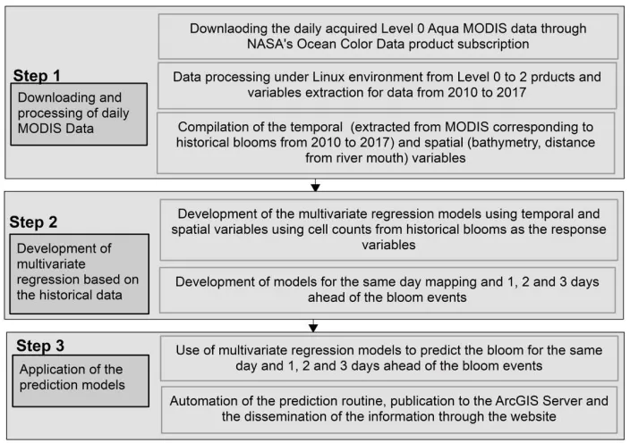
Figure 2. Three-step workflow established for HAB mapping and forecasting 2.1. Step 1
The first step involved the identification of temporal ocean color products and spatial variables that could control, or correlate with, the distribution of algal blooms in general and/or the HAB in the study area (in our case K. brevis). The selection of these variables was largely based on reported findings from similar settings elsewhere and, to a lesser extent, on our observations.
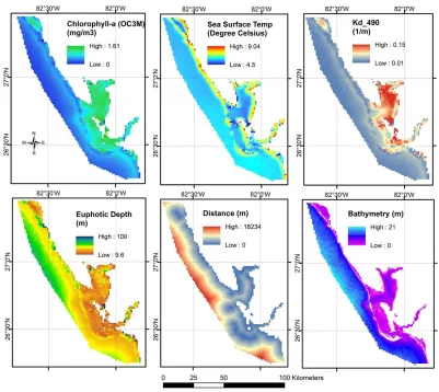
This step involved automatic downloading and processing of daily ocean color data products acquired by the National Aeronautics and Space Administration (NASA) MODIS Aqua satellite. NASA’s ocean color processing website (https://oceancolor.gsfc.nasa.gov/) provides an option for periodical data downloads for specified regions via a free data subscription service. We specified southwestern Florida as the study area, Aqua MODIS data as the data type, and a daily data download for frequency. The automatic data download was scheduled using the task scheduling programs available within the Linux environment. The downloaded Level 0 product was processed to Level 1 and later to Level 2 using NASA’s SeaDAS 7.4 software to extract relevant temporal variables. A total of 13 ocean color data products were downloaded and processed. These products include euphotic depth, the ocean chlorophyll three-band algorithm for MODIS (chlorophyll-a OC3M), chlorophyll-a Generalized Inherent Optical Property (GIOP), chlorophyll-a Garver-Siegel- Maritorena (GSM), fluorescence line height (Flh), a diffused attenuation coefficient for downwelling irradiance at 490 nm (Kd_490), a particulate backscattering coefficient at 547 nm (bbp_547_giop), turbidity index, sea surface temperature (SST), wind direction, wind speed, colored dissolved organic material (CDOM) [26] and Secchi disk depth (Zsd morel) [27]. Additional spatially relevant variables were considered, as well. Our preliminary inspection of these products revealed large and rapid variations in chlorophyll-a content, SST, the attenuation coefficient, and euphotic depth in proximity to the shoreline and to the freshwater outlets (river mouth; Figure 3), thus suggesting that bathymetry and distance from the river mouth should be incorporated in the model’s development.
The collected ocean color data products were later checked for consistency and significance. Discontinuous data were not considered. For example, the data for colored dissolved organic matter (CDOM) concentration was found to be discontinuous and patchy over the investigated period (2010 to 2017) and was thus omitted from the list of potential variables considered for model development.
(redundant variables) were identified using the extracted Variance Inflation Factor (VIF) [28] values. A variable with a VIF value exceeding 7.5 was considered redundant with the second highest VIF value. In cases where multiple variables were identified as being redundant, the significant variables were retained and the insignificant ones were omitted. Using water clarity measurements as an example, Secchi disk depth was found to be redundant with euphotic depth, and the former was found to be less significant and was dropped. Following the omission of redundant variables, the multivariate regression was run again to make sure the R-square value and model’s significance did not decrease. The overall target of this iterative exercise was to obtain the highest R-square value with a minimal number of significant variables. Only13 of the initial 15 variables were considered for model construction. The spatial and temporal variables included in the model are explained below.
2.1.1. Euphotic Depth (m)
The euphotic depth represents the depth at which 1% of the light incident on the ocean’s surface can reach [29–31]. This depth provides a measure of the depth where light penetrates, nutrients and algae diminish, and productivity decreases [32]. Water bodies with low euphotic depths generally have a high nutrient content, are more productive and eutrophic [33], and provide favorable conditions for HAB development [34]. The euphotic depth was calculated using the technique documented in a previous study [30].
2.1.2. Wind direction (degrees) and wind speed (m/s)
The wind direction and speed can affect the distribution of algal blooms in three major ways: (1) prevailing wind directions create ocean currents and water exchanges that transport HAB cells [35,9] or their biotoxins [9], (2) wind combined with ocean bathymetry controls the locations where nutrient upwelling occurs; HABs feed on and concentrate around these nutrient upwelling sites [13], and (3) winds can also transfer the aerosols on the sea surface [21] that were shown as promoting the growth of toxic phytoplankton [36]. The wind direction and wind speed were calculated using a reflectance model based on the Cox-Mux wave-slope distribution [37].
2.1.3. Chlorophyll-a (mg/m3)
The concentration of chlorophyll-a provides direct measurements of the growth of the algae in aquatic environments [38]. Three different types of algorithms were used to compute the chlorophyll-a content: chlorophyll-chlorophyll-a OC3M (ocechlorophyll-an chlorophyll three-bchlorophyll-and chlorophyll-algorithm for MODIS, [39]), chlorophyll-a GSM (Garver-Siegel- Maritorena, [40]) and chlorophyll-a GIOP (Generalized Inherent Optical Property, [41]). These algorithms provide estimates for phytoplankton biomass [42] in coastal waters and have been validated for consistency and accuracy with field observations in different parts of the world [43–46]. An increased chlorophyll-a concentration has been taken as a strong indicator of HAB distribution [47,48], and chlorophyll-a OC3M data has been used for detecting HAB along the west coast of Florida [20]. All three types of chlorophyll-a measurements were considered in this study as they were found to be correlated with algal cell count during the exploratory multivariate regression.
2.1.4. Diffuse Attenuation Coefficient
through in situ measurement [53]. The diffuse attenuation coefficient was calculated using the technique described in a previous study [50].
2.1.5. Turbidity Index
The turbidity index provides a measure for the clarity of the water through the scattering of light caused by suspended particles [54,55]. Spatial and temporal variations of turbidity in water bodies has been successfully used to identify phytoplankton blooms [56,57]. Although a turbidity index is not a direct indicator of HAB occurrences, it has been successfully used to estimate the severity of a HAB once it was independently detected [58]. The turbidity index was calculated using procedures described in a previous study [59].
2.1.6. Particulate Backscattering Coefficient at 547 nm
This is the backscattering coefficient of particles at 547 nm. The backscattering coefficient as determined by satellite sensors and in situ measurements has been used in the past to identify the distribution of HABs. A research study [60] employed satellite-based and underwater glider measurements of the backscattering coefficient at 547 nm to detect K. brevis blooms in the Gulf of Mexico and verified their findings by in situ observations. A backscattering coefficient at 551 nm extracted from a Visible Infrared Imaging Radiometer Suite (VIIRS) sensor, which is analogous to the MODIS backscattering coefficient at 547 nm, was used in conjunction with fluorescence data to detect the K. brevis bloom at the West Florida shelf [61]. In the same area, in situ measurements of the backscattering coefficient at 551 nm and chlorophyll data were successfully used to detect a K. brevis bloom [62]. The backscatter coefficient of particles at 547 nm was calculated using an algorithm available in the literature [63,64].
2.1.7. Sea Surface Temperature (°C)
SST influences phytoplankton productivity in multiple ways: (1) individual biological species including algal blooms thrive under different and specific temperature regimes, and (2) the availability and solubility of many biochemical materials needed for their growth and development is temperature dependent [65,35]. Many studies have shown a correlation between SST and algal bloom distributions in the Mediterranean Basin [66], Kuwait Bay [67,68] and on a global scale [69]. The productivity of K. brevis increases in the fall and early spring at the west Florida shelf primarily because of the ideal temperature conditions during these time periods [19]. Increased SST was found to be conducive to HAB development in the coastal waters of Oman [70] and in Gulf of Mexico [71].
2.1.8. Fluorescence Line Height (FLH)
The fluorescence line height (FLH) is a relative measure of the amount of radiance leaving the sea surface in the chlorophyll fluorescence emission band [72]. FLH has been successfully used in the detection of chlorophyll in several studies [22,23,25]. Similarly, FLH was used in a study [19] to detect chlorophyll-a concentration in the coastal waters of southwestern Florida. A review of previous studies showed a positive correlation between the MODIS-derived fluorescence and chlorophyll-a concentration in ocean waters with algal blooms [72]. More recently, an in situ measurement of FLH was used in conjunction with the backscattering coefficient to map the distribution of K. brevis in the Gulf of Mexico [60]. Similarly, FLH derived from VIIRS was used to detect K. brevis blooms at the West Florida Shelf [61]. A normalized FLH chlorophyll-related radiance (mW cm-2 µm-1 sr-1) was
generated using a previously established algorithm [73].
2.1.9. Bathymetry (m)
shelf systems and coastal areas in general, are considered to be vulnerable to HAB occurrences due to the accumulation of biomass [76]. Bathymetric data acquired from USGS (https://coastal.er.usgs.gov/flash/bathy-entireFLSH.html) were used as one of the spatial variables.
2.1.10. Distance from the river mouth (m)
Riverine organics are major sources of nutrients for the West Florida Shelf of the Gulf of Mexico [77]. The riverine discharge provides high nutrient loads [78] that largely control the phytoplankton population and eutrophication around the river discharge locations and adjoining estuarine systems [79,80]. The distance from the mouth of the river was computed using the Euclidean Distance function in ArcGIS.
Figure 3. Mean values for the significant variables including chlorophyll-a (OC3M), SST, diffuse attenuation coefficient, and euphotic depth calculated from MODIS products acquired throughout the period 2010 to 2017 over the study area. The distance from river mouth and bathymetry data are also shown.
2.2. Step 2
magnitude. Such variations, if not accounted for, could affect model outputs. For each inventoried location, we extracted the values of the normalized input variables.
Four regression models were constructed: (i) same-day, (ii) one day in advance, (iii) two days in advance, and (iv) three days in advance. For each of the models, data were divided into training (80%) and testing (20%) datasets. The training data were used to develop the regression, and the accuracy assessment was done on the testing datasets. For the same-day model, the regression was conducted on 80% of the reported HABs occurrences (102 unique-day bloom events) against the variables on bloom days (days when blooms were reported). For the one day in advance model, the regression was conducted for the response versus the variables acquired one day in advance of the bloom day. Similarly, for the two-day and three-day in advance models, the response was regressed against the variables acquired two and three days in advance, respectively. Each of the four models had its individual datasets (response and variables) for regression and validation. Predictive models (ii, iii, and iv) were designed to capture the onset of the HABs in contrast to those that developed days earlier and continued in the following days. To this end, a bloom reported on dayn was excluded from
the one-day advance dataset if another was reported in the same location in dayn-1. Similarly, a bloom
reported on dayn was excluded from the two-day dataset if another was reported in the same location
in dayn-1 or dayn-2 and from the three-day dataset if a bloom was reported on dayn-1, dayn-2 or daysn-3.
The cell count responses from the models were lumped into three groups: (i) no bloom (cell count ≤ 300 per/liter), (ii) low concentration (cell count > 300 and < 10,000 per liter) and (iii) high concentration (cell count ≥10,000 per liter). We adopted the threshold values used by the Harmful Algal Bloom Observation System (https://habsos.noaa.gov/) in categorizing cell counts for consistency purposes and to facilitate comparisons with NOAA’s observations. The multivariate regression model was developed for each group of the data. For any new satellite data for any specific day, a respective regression was used to predict the HAB on the same day and 1, 2 and three days in advance of the potential HAB occurrence.
2.3. Step 3
The generated regression equations were utilized for same-day mapping and one-, two- and three-day advance predictions of HAB. The regression models were developed for three bloom lag periods and applied to the collective set of variables. The results (same-day mapping and one-, two- and three-day advance prediction of HAB) are published on our website (http://www.esrs.wmich.edu/webmap/bloom/) using the ArcGIS server and ArcGIS API for JavaScript. The MODIS data for every day is acquired at ~4 pm, is made available for download on NASA’s website at ~5 pm, and is processed for HAB occurrences and published on our website at ~10 pm. This process was coded in Python 2.7 to allow the program to run automatically at the same time every day.
3. Results and Discussions
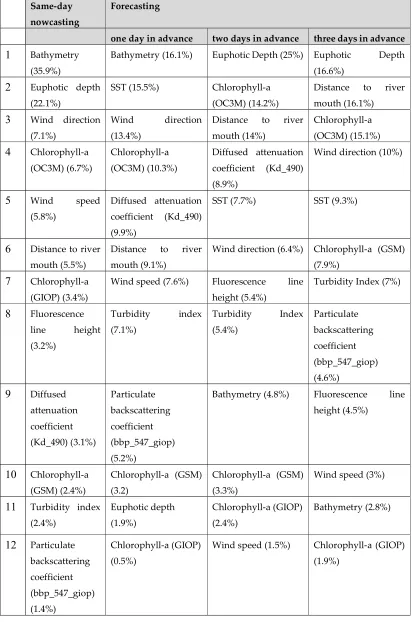
The prediction was done in two phases: (a) nowcasting and (b) one, two and three days in advance forecasting. The model outputs are provided in Tables 1 and 2. Table 1 lists the selected variables with their relative significance (in percentage) for the same-day and the one-, two- and three-day predictions. Table 2 provides the multivariate regression coefficients for each of the selected variables for the same-day and the one-, two- and three-day predictions. The sign (+/-) in front of the coefficient for each variable indicates the nature (positive/negative) of the relationship between the variable in question and the response. The logarithm (base 10) of cell count was used as the response variable. A cell count exceeding 300 per liter was considered to indicate the presence of a HAB.
The information provided in Tables 1 and 2 can be used to interpret the nature of the relationship between HAB occurrences and the individual variables, determine the directionality (negative or positive) of the relationship, and evaluate the comparative significance of these relationships.
variable as presented in Table 1. For the one-day forecasting, bathymetry, SST, wind direction, chlorophyll-a (OC3M), and diffused attenuation coefficient (KD_490) were found to have a 65% contribution to the response variable. For the two-day forecasting, euphotic depth, chlorophyll-a (OC3M), distance to river mouth, diffused attenuation coefficient (KD_490) and SST were found to have 69% contribution to the response variables. The euphotic depth, distance to river mouth, chlorophyll-a (OC3M), wind direction and SST had a 67% contribution to the response variable for the three-day forecasting.
A 1:1 correspondence in the ranking and significance of variables in the four models should not be expected given that the variables could have varying lag time effects on HAB development. For example, a study [81] found a positive correlation between algal bloom events and nitrate and ammonium concentrations as early as five days prior to the bloom. Similarly, a study [82] found a positive correlation between HAB occurrences and temperature and aerosols particle distribution, which are the air-borne sources of phosphate, iron and trace elements in the East China Sea. Higher concentrations of phosphorous and iron above the threshold did not correlate with the HAB events because these are limiting nutrients for HAB growth. The increase in concentration of nitrogen, however, correlated with the HAB concentration. The lag time between the spike in the nitrogen concentration in the aerosols and HAB event was two days. Similarly, in the coastal waters of Charlotte County, one can attribute the significance and high ranking of some variables (distance to river mouth, and chlorophyll-a) in our two- and three-day predictive models to the presence of a two day lag time for nutrients in rivers to reach the coastal waters and induce HABs.
An inspection of Tables 1 and 2 reveals differences in the rankings and significance of the variables between the four solutions. However, there are multiple variables that appear to be significant (≥ significance 5%) for three or more of the four solutions. These include chlorophyll-a (4 models: 6 to 15%), Euphotic depth (same-day: significance [S] 22.1%, rank [R]2nd; two-days: S 25%, R
1st; three-days: S 16.6%, R 1st), SST (one-day: S 15.5%, R 2nd; two-days: S 7.7%, R 5th; three-days: S 9.3%,
R 5th); wind direction (same-day: S 7.1%, R 3rd; one-day: S 13.4%, R 3rd; two-days: S 6.4%, R 6th;
three-days: S 10%, R 4th), Chlorophyll-a OC3M (same-day: S 6.7%, R 4th; one-day: S 10.3%, R 4th; two-days:
S 14.2%, R 2nd; three-days: S 15.1%, R 3rd), distance to river mouth (same-day: S 5.5%, R 6th; one-day:
S 9.1%, R 6th; two-days: S 14%, R 3rd; three-days: S 16.1%, R 2nd) and turbidity index (one-day: S 7.1%,
R 8th; two-days: S 5.4%, R 8th; three-days: S 7%, R 7th). Other variables appear to be consistently less
important (significance <5%) in 3 or more of the model outputs. These include bathymetry, wind speed, chlorophyll-a GIOP, fluorescence line height, diffused attenuation coefficient (Kd_490), chlorophyll-a GSM and particulate backscattering coefficient (bbp_547_giop).
Shallow bathymetry seems to be a significant factor for same-day predictions (S 35.9%; R 1st;
Table 1), but its significance correlates negatively with the prediction period (one-day: S 16.1%, rank: 1st; two-days: S 4.8%, R 9th; three-days: S 2.8%, R 11th, Table 1). The association of HABs with shallow
bathymetry was inferred from the –ve sign of the coefficient for the bathymetry variable for the same day. Similarly, the association of HABs with increasing euphotic depth and turbidity is inferred from the +ve sign for the coefficient for these two variables (euphotic depth and turbidity index) in each of the four models. The chlorophyll-a (OC3M) content shows a positive correlation with bloom occurrences and a positive correlation with prediction periods (sameday: S: 6.7%, coefficient= -0.2662; one-day: S: 10.3%, coefficient: 0.0609; two-days: S: 14.2%; coefficient=0.0874; and three-days: S: 15.1%, coefficient: 0.1326). A positive correlation is observed for the bloom occurrences with wind direction for all lag times, but the significance and rank varies for the investigated models (S: 13.4% to 6.4%; R: 3rd to 6th). The diffused attenuation coefficient seems to have a positive correlation
coefficient (same-day: 2.6613; one-day: 5.2936; two-days: 6.2945; and three-days: 1.0121) and an increasing significance and/or higher rank going from the same day (S 3.1%, R 9th) to one-day (S 9.9%;
R 5th), and two-days (S 8.9%, R 4th), but its effect diminishes in three days (S 1.3%, R 13th). SST seems
to be less significant on the day of the bloom (S 0.8%; R 13th) compared to the one-day (S 15.5%, R 2nd),
two-days (S 7.7%, R 5th)and three-days (S 9.3%, R 5th) advanced predictions. Blooms occur at cooler
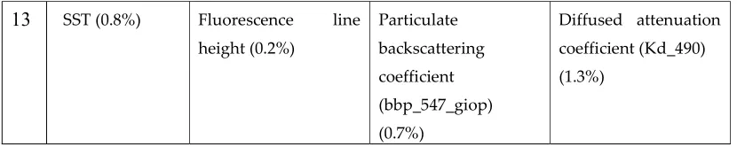
Table 1. Selected variables with their relative significance (in percentage) for same-day nowcasting, and one-, two- and three-day predictions.
Same-day nowcasting
Forecasting
one day in advance two days in advance three days in advance
1
Bathymetry (35.9%)Bathymetry (16.1%) Euphotic Depth (25%) Euphotic Depth (16.6%)
2
Euphotic depth (22.1%)SST (15.5%) Chlorophyll-a (OC3M) (14.2%)
Distance to river mouth (16.1%)
3
Wind direction(7.1%)
Wind direction (13.4%)
Distance to river mouth (14%)
Chlorophyll-a (OC3M) (15.1%)
4
Chlorophyll-a(OC3M) (6.7%)
Chlorophyll-a (OC3M) (10.3%)
Diffused attenuation coefficient (Kd_490) (8.9%)
Wind direction (10%)
5
Wind speed(5.8%)
Diffused attenuation coefficient (Kd_490) (9.9%)
SST (7.7%) SST (9.3%)
6
Distance to river mouth (5.5%)Distance to river mouth (9.1%)
Wind direction (6.4%) Chlorophyll-a (GSM) (7.9%)
7
Chlorophyll-a (GIOP) (3.4%)Wind speed (7.6%) Fluorescence line height (5.4%)
Turbidity Index (7%)
8
Fluorescence line height (3.2%)Turbidity index (7.1%)
Turbidity Index (5.4%) Particulate backscattering coefficient (bbp_547_giop) (4.6%)
9
Diffused attenuation coefficient (Kd_490) (3.1%) Particulate backscattering coefficient (bbp_547_giop) (5.2%)Bathymetry (4.8%) Fluorescence line height (4.5%)
10
Chlorophyll-a (GSM) (2.4%)Chlorophyll-a (GSM) (3.2)
Chlorophyll-a (GSM) (3.3%)
Wind speed (3%)
11
Turbidity index (2.4%) Euphotic depth (1.9%) Chlorophyll-a (GIOP) (2.4%) Bathymetry (2.8%)12
Particulate backscattering coefficient (bbp_547_giop) (1.4%) Chlorophyll-a (GIOP) (0.5%)13
SST (0.8%) Fluorescence line height (0.2%)Particulate backscattering coefficient (bbp_547_giop) (0.7%)
Diffused attenuation coefficient (Kd_490) (1.3%)
Table 2. Multivariate regression coefficients for each variable in predicting HABs for same-day mapping, and one-, two- and three-day advanced predictions.
Variables Coefficients
Same-day one day in
advance
two days in advance
three days in advance
Bathymetry (m) -0.2662 0.0609 0.0874 0.1326
Euphotic Depth (m) 0.0296 0.0022 0.0231 0.0189
Wind Direction (degrees) 216.5790 270.1179 162.3239 287.9521
Chlorophyll-a (OC3M) (mg/m3) 0.5120 0.5418 0.9005 1.0869
Wind Speed (m/s) -250.5957 214.0178 53.2687 119.2459
Distance to Mouth of River (m) -0.1593 0.0001 0.0001 0.0001
Chlorophyll-a GIOP (mg/m3) 0.2617 0.0044 0.1549 -0.1380
Normalized Fluorescence Line Height
(mWcm-2 um-1 sr-1) -395.2367 0.0001 -551.1232 -514.3536
Diffused Attenuation Coefficient (m-1) 2.6613 5.2936 6.2945 1.0121
Chlorophyll-a GSM (mg/m3) 0.1845 0.1417 0.2116 0.5693
Turbidity Index 73.0929 143.0333 135.8686 202.1670
Particulate Backscattering Coefficient (m-1) 4287.9827
-12551.1376 -1854.9512 -3779.3400
SST (°C) -0.0188 -0.2164 -0.1514 -0.2002
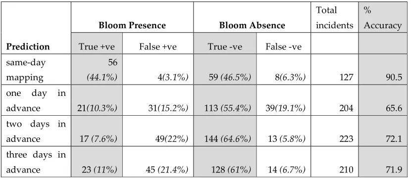
The assessment of the performance of the four models is presented in Table 3. The accuracy of the same day was the highest (90.5%), and the accuracies of the one-day, two-day, and three-day prediction models were assessed at 65.6%, 72.1%, and 71.9%, respectively.
Table 3. Assessment of the accuracy of the generated multivariate models (same-day mapping and one-, two- and three-day advanced predictions). The relative percentage for each category is presented in parentheses.
Prediction
Bloom Presence Bloom Absence
Total incidents
% Accuracy
True +ve False +ve True -ve False -ve same-day
mapping
56
(44.1%) 4(3.1%) 59 (46.5%) 8(6.3%) 127 90.5 one day in
advance 21(10.3%) 31(15.2%) 113 (55.4%) 39(19.1%) 204 65.6 two days in
advance 17 (7.6%) 49(22%) 144 (64.6%) 13 (5.8%) 223 72.1
three days in
advance 23 (11%) 45 (21.4%) 128 (61%) 14 (6.7%) 210 71.9
5. Conclusions, Limitations, and Applications
The study focused on developing an early warning system for K. brevis-related HABs off the coast of South Florida. We used historical field HAB data from 2010 to 2017 to develop a multivariate regression and determine the significance of the variables for different prediction scenarios. The prediction system involved the same-day nowcasting method and forecasting for one, two and three days in advance of the onset of the bloom. The same-day nowcasting provided 90% accuracy, whereas the one, two and three days in advance forecasting provided 65, 72 and 71%s accuracies, respectively. The investigation took advantage of ocean color data to develop methodologies and procedures that may enhance decision making processes, improve citizens’ quality of life, and strengthen the local economy. Even though this project focuses on the K. brevis related HAB in Charlotte County and its surrounding neighbors, the model can be replicated for other species and can be applied in other areas. The prediction system can be utilized to plan uses of coastal waters for recreational purposes and other environmental services. Monitoring the extent and intensity of HABs could be used to improve the environmental and socioeconomic status of this area and develop long-term environmental programs and policies.
There are several limitations with the current use of MODIS data. There can be differences between the time a bloom was reported and the time it was captured by satellite imagery, and during that time the algae could move laterally and vertically in the water column. Our approach assumes that the algae are stationary. Diurnal algae variations are not captured by the MODIS imagery. In field controlled and natural environments, a previous study [83] showed a decrease in fluorescence before reaching the maximum value under natural photosynthetically available radiation, while another study [84] reported diurnal variations in algae populations in the surface and in the mid-column. Similar diurnal variations were reported for K. brevis in the West Florida Shelf [85].
halted on cloudy days. Due to the weather dependency of the temporal variables, it is difficult to develop models that include multiple variables with varying time lags. Additionally, with the coarse spatial resolution of MODIS derived variables (e.g., SST: 1000 m; turbidity index: 500), the detection of HABs within a small area is limited.
The developed models lack real time measurements for nutrients in surface and groundwater due to the absence of continuous monitoring systems in our study area. Instead, we have proxies (e.g., euphotic depth and turbidity indices) that can account for the nutrient content in the aquatic system. The predictability of the developed models could be improved with the inclusion of direct and daily measurements of nitrate and phosphate in surface water that automatically feed the data into the model. The current problem of discontinuous and coarse resolution of the MODIS data could be addressed if it was replaced by Unmanned Aerial Vehicles (UAVs) datasets. UAVs acquire high resolution images devoid of atmospheric influences. These new data acquisition systems could increase the accuracy, predictability and replicability of our model in Charlotte County and elsewhere in the world. These methods would enable the construction of robust models that account for varying lag times and produce continuous high spatial and temporal resolution prediction maps.
Supplementary Materials: The website developed for this project is available at: http://www.esrs.wmich.edu/webmap/bloom
Author Contributions: Sita Karki processed the remote sensing data, developed the model and prepared the manuscript. Mohamed Sultan advised the project from the beginning to the end and helped in the manuscript development. Racha Elkadiri guided the remote sensing data processing and supported the model development. Tamer Elbayoumi provided the statistical framework and the analysis for the project.
Funding: The project was supported through the Enterprise Charlotte Foundation, and internal funding was provided by Western Michigan University.
Acknowledgments: The authors would like to thank Charlotte County staff for their invaluable input. Conflicts of Interest: The authors declare no conflict of interest.
References
1. Glibert, P.M.; Harrison, J.; Heil, C.; Seitzinger, S. Escalating worldwide use of urea—a global change contributing to coastal eutrophication. Biogeochemistry2006, 77, 441–463, doi:10.1007/s10533-005-3070-5.
2. Howarth, R.W.; Billen, G.; Swaney, D.; Townsend, A.; Jaworski, N.; Lajtha, K.; Downing, J.A.; Elmgren, R.; Caraco, N.; Jordan, T.; Berendse, F.; Freney, J.; Kudeyarov, V.; Murdoch, P.; Zhu, Z.L. Regional nitrogen budgets and riverine inputs of N and P for the drainages to the North Atlantic Ocean: natural and human influences. Biogeochemistry1996,35, 75–139.
3. Landsberg, J.H. The effects of harmful algal blooms on aquatic organisms. Rev. fish. sci. aquac.2002, 10, 113–390, doi:10.1080/20026491051695.
4. Fleming, E.; Kirkpatrick, C.; Backer, L.; Walsh, C.J.; Nierenberg, K.; Clark, J. et al. Review of Florida red tide and human health effects. Harmful Algae2011, 10, 224–233, doi:10.1016/j.hal.2010.08.006.
5. Steidinger, K.A.; Vargo, G.A.; Tester, P.A.; Tomas, C.R. Bloom dynamics and physiology of Gymnodinium breve with emphasis on the Gulf of Mexico. In Physiological Ecology of Harmful Algal Blooms, 1st ed.; Anderson, D.M, Cambella, A.D, Hallegraeff, G.M., Eds.; Springer-Verlag: Heidelberg, Germany, 1998; pp. 133–154, ISBN 3540641173.
7. Thyng K.M.; Hetland R.D.; Ogle M.T.; Zhang, X.; Chen, F.; Campbell, L. Origins of Karenia brevis
harmful algal blooms along the Texas coast. Limnol. Oceanogr Fluids Environ.2013, 3, 269–278, doi:10.1215/21573689-2417719.
8. Evans, G.; L. Jones. Economic impact of the 2000 red tide on Galveston County, Texas: A case study, Austin, TX, USA, 2001.
9. Raine, R.; McDermott, G.; Silke, J.; Lyons, K.; Nolan, G.; Cusack, C. A simple short range model for the prediction of harmful algal events in the bays of southwestern Ireland. J. Mar. Syst. 2010, 83, 150– 157, doi:10.1016/j.jmarsys.2010.05.001.
10. Cha, Y.; Park, S.S.; Kim, K.; Byeon, M.; Stow, C.A. Probabilistic prediction of cyanobacteria abundance in a Korean reservoir using a Bayesian Poisson model. Water Resour. Res. 2014,50, 2518–2532,
doi:10.1002/2013WR014372.
11. Harred, L.B.; Campbell, L. Predicting harmful algal blooms: a case study with Dinophysis ovum in the Gulf of Mexico. J. Plankton Res. 2014, 36, 1434–1445, doi:10.1093/plankt/fbu070.
12. McGillicuddy, D.J.; Anderson, D.M.; Lynch, D.R.; Townsend, D.W. Mechanisms regulating large-scale seasonal fluctuations in Alexandrium fundyense populations in the Gulf of Maine: Results from a physical–biological model. Deep Sea Res. Part II Top. Stud. Oceanogr.2005, 52, 2698–2714, doi:10.1016/j.dsr2.2005.06.021.
13. Cusack, C.; Dabrowski, T.; Lyons, K.; Berry, A.; Westbrook, G.; Salas, R.; Duffy, C.; Nolan, G.; Silke, J. Harmful Algal Bloom forecast system for SW Ireland. Part II: Are operational oceanographic models useful in a HAB warning system? Harmful Algae2016, 53, 86–101, doi:10.1016/j.hal.2015.11.013.
14. Aleynik, D.; Dale, A.C.; Porter, M.; Davidson, K. A high resolution hydrodynamic model system suitable for novel harmful algal bloom modelling in areas of complex coastline and topography.
Harmful Algae2016, 53, 102–117, doi:10.1016/j.hal.2015.11.012.
15. Gillibrand, P.A.; Siemering, B.; Miller, P.I; Davidson, K. Individual-based modelling of the development and transport of a Karenia mikimotoi bloom on the North-West European continental shelf. Harmful Algae2016, 53, 118–134, doi:10.1016/j.hal.2015.11.011.
16. Stumpf, R.P.; Litaker, R.W.; Lanerolle, L.; Tester, P.A. Hydrodynamic accumulation of Karenia off the West Coast of Florida. Cont. Shelf Res.2008, 28, 189–213, doi:10.1016/j.csr.2007.04.017.
17. Turrell, E.; Stobo, L.; Lacaze, J.P.; Bresnan, E.; Gowland, D. Development of an ‘early warning system’ for harmful algal blooms using solid-phase adsorption toxin tracking (SPATT). OCEANS 2007-Europe
2007, 1–6, doi:10.1109/OCEANSE.2007.4302436.
18. Lee, J.H.W.; Hodgkiss, I.J.; Wong, K.T.M.; Lam, I.H.Y. Real time observations of coastal algal blooms by an early warning system. Estuar. Coast Shelf Sci. 2005, 65, 172–190, doi:10.1016/j.ecss.2005.06.005.
19. Hu, C.; Muller-Karger, F.E.; Taylor, C.; Carder, K.L.; Kelble, C.; Johns, E.; Heil, C.A. Red tide detection and tracing using MODIS fluorescence data: a regional example in SW Florida coastal waters.
Remote Sens. Environ.2005, 97, 311–321, doi:10.1016/j.rse.2005.05.013.
20. Carvalho, G.A.; Minnett, P.J.; Fleming, L.E.; Banzon, V.F.; Baringer, W. Satellite remote sensing of harmful algal blooms: A new multi-algorithm method for detecting the Florida Red Tide (Karenia brevis). Harmful algae2010, 9, 440–448, doi:10.1016/j.hal.2010.02.002.
22. Neville, R.A.; Gower, J.F.R. Passive remote sensing of phytoplankton via chlorophyll fluorescence. J. Geophys. Res. 1977, 82, 3487–3493, doi:10.1029/JC082i024p03487.
23. Pan, D.L.; Gower, J.F.R; Lin, S.R. A study of band selection for fluorescence remote sensing of ocean chlorophyll-a. Oceanol. Limnol. Sin. 1989, 20, 564–570.
24. Fischer, J.; Kronfeld, U. Sun-stimulated chlorophyll fluorescence: 1. Influence of oceanic properties. Int J Remote Sens. 1990, 11, 2125–2147, doi:10.1080/01431169008955166.
25. Hoge, F.E.; Lyon, P.E.; Swift, R.N.; Yungel, J.K.; Abbott, M.R.; R.M. Letelier, R.M.; W.E. Esaias, W.E. Validation of Terra-MODIS phytoplankton chlorophyll fluorescence line height. I. Initial airborne lidar results. Appl. Optics2003, 42, 2767–2771, doi:10.1364/AO.42.002767.
26. Morel, A.; Gentili, B. A simple band ratio technique to quantify the colored dissolved and detrital organic material from ocean color remotely sensed data. Remote Sens. Environ.2009, 113, 998–1011, doi:10.1016/j.rse.2009.01.008.
27. Tyler, J.E. The Secchi disk. Limnol. Oceanogr. 1968, 13, 1−6, doi:10.4319/lo.1968.13.1.0001.
28. O’Brien, R.M.A. Caution regarding rules of thumb for Variance Inflation Factors. Qual. Quant.2007,
41, 673–690, doi:10.1007/s11135-006-9018-6.
29. Kirk, J.T.O. Light and Photosynthesis in Aquatic Ecosystems, 2nd ed.; Cambridge University Press: New York, NY, USA, 1994; ISBN 0521459664.
30. Morel, A.; Huot, Y.; Gentili, B.; Werdell, P.J.; Hooker, S.B.; Franz, B.A. Examining the consistency of products derived from various ocean color sensors in open ocean (Case 1) waters in the perspective of a multi-sensor approach. Remote Sens. Environ.2007, 111, 69−88, doi:10.1016/j.rse.2007.03.012.
31. Ryther, J.H. Photosynthesis in the Ocean as a Function of Light Intensity. Limnol. Oceanogr. 1956, 1, 61–70, doi:10.4319/lo.1956.1.1.0061.
32. Behrenfeld, M.J.; Falkowski, P.G. A consumer’s guide to phytoplankton primary productivity models.
Limnol. Oceanogr. 1997, 42, 1479– 1491, doi:10.4319/lo.1997.42.7.1479.
33. Behrenfeld, M.J.; Boss, E; Siegel, D.A.; Shea, D.M. Carbon-based ocean productivity and phytoplankton physiology from space. Global Biogeochem. Cycles2005, 19, GB1006, doi:10.1029/2004GB002299.
34. Anderson, D.M.; Glibert, P.M.; Burkholder, J.M. Harmful algal blooms and eutrophication: nutrient sources, composition, and consequences. Estuaries Coast2002, 25, 704–726, doi:10.1007/BF02804901.
35. Edwards, A.; Jones, K.; Graham, J.M; Griffiths, C.R; MacDougall, N.; Patching, J.; Richard, J.M; Raine, R. Transient coastal upwelling and water circulation in Bantry Bay, a ria on the SW coast of Ireland.
Estuar. Coast. Shelf Sci. 1996,42, 213–230, doi:10.1006/ecss.1996.0016.
36. Al Shehhi, M.R.; Gherboudj, I.; Ghedira, H. Temporal-spatial analysis of chlorophyll concentration associated with dust and wind characteristics in the Arabian Gulf. OCEANS – Yeosu: IEEE2012, 1-6, doi:10.1109/OCEANS-Yeosu.2012.6263404.
37. Cox, C.; Munk, W. The measurements of the roughness of the sea surface from photographs of the sun’s glitter. J. Opt. Soc. Amer. 1954,44, 838–850, doi:10.1364/JOSA.44.000838
38. Baban, S.M.J. Trophic classification and ecosystem checking of lakes using remotely sensed information. Hydrol. Sci. J.1996, 41, 939–957, doi:10.1080/02626669609491560.
series, SeaWiFS postlaunch calibration and validation analyses, part 3; Hooker, S. B., Firestone, E. R., Eds.; NASA Goddard Space Flight Center: Greenbelt, Maryland, USA, 2000; Volume 11, pp. 9–23.
40. Maritorena, S.; Siegel, D.A.; Peterson, A.R. Optimization of a semi- analytical ocean color model for global-scale applications. Appl. Opt. 2002, 41, 2705–2714, doi:10.1364/AO.41.002705.
41. Franz, B.A.; Werdell, P.J.A generalized framework for modeling of inherent optical properties in ocean remote sensing applications. In Proceedings of Ocean Optics, Anchorage, Alaska, USA, 2010.
42. Tilstone, G.H.; Lotliker, A.A.; Miller, P.I.; Ashraf, P.M.; Kumar, T.S.; Suresh, T.; Ragavan, B.; Menon, H.B. Assessment of MODIS-Aqua chlorophyll-a algorithms in coastal and shelf waters of the eastern Arabian Sea. Cont. Shelf Res. 2013, 65, 14–26, doi:10.1016/j.csr.2013.06.003.
43. Campbell, J.W.; Feng, H. The empirical chlorophyll algorithm for MODIS: testing the OC3M algorithm using NOMAD data. In Ocean Color Bio-optical Algorithm Mini-workshop, New England Center, USA, 27–29 September; University of New Hampshire: Dunham, USA, 2005, pp. 1–9.
44. Hattab, T.; Jamet, C.; Sammari, C.; Lahbib, S. Validation of chlorophyll-a concentration maps from Aqua MODIS over the Gulf of Gabes (Tunisia): comparison between MedOC3 and OC3M bio-optical algorithms. Int. J. Remote. Sens.2013,34, 7163–7177, doi:10.1080/01431161.2013.815820.
45. Komick, M.; Costa, M.; Gower, J. Bio-optical algorithm evaluation for MODIS for western Canada coastal waters: An exploratory approach using in situ reflectance. Remote Sens. Environ.2009, 113, 794– 804, doi:10.1016/j.rse.2008.12.005.
46. Shang, S.L.; Dong, Q.; Hu, C.M.; Lin, G.; Li, Y.H.; Shang, S.P. On the consistency of MODIS chlorophyll a products in the northern South China Sea, Biogeosciences2014,11, 269–280, doi:10.5194/bg-11-269-2014.
47. Tang, D.L.; Di, B.P.; Wei, G.; Ni, I.H.; Oh, I.S.; Wang, S.F. Spatial, seasonal and species variations of harmful algal blooms in the South Yellow Sea and East China Sea. Hydrobiologia2006, 568, 245–253, doi:10.1007/s10750-006-0108-1.
48. Wei, G.; Tang, D.L.; Wang, S. Distribution of chlorophyll and harmful algal blooms (HABs): A review on space based studies in the coastal environments of Chinese marginal seas. Adv Space Res. 2008, 41, 12–19, doi:10.1016/j.asr.2007.01.037.
49. Austin, R.W.; Petzold, T.J. The determination of the diffuse attenuation coefficient of sea water using the Coastal Zone Color Scanner. In Oceanography from Space, Marine Sciences, 1st ed.;Gower, J.F.R., Ed.; Springer: Boston, MA, USA, 1981; Volume 13, pp. 239–256,ISBN978-1-4613-3317-3.
50. Lee, Z-P.; Du, K-P.; Arnone, R. A model for the diffuse attenuation coefficient of downwelling irradiance. J. Geophys. Res.2005, 110,C02016, doi:10.1029/2004JC002275.
51. Chen, J.; Cui, T.; Tang, J.; Song, Q. Remote sensing of diffuse attenuation coefficient using MODIS imagery of turbid coastal waters: A case study in Bohai Sea, Remote Sens. Enviro. 2014, 140, 78–93, doi:10.1016/j.rse.2013.08.031.
52. Ghanea, M.; Moradi, M.; Kabiri, K. A novel method for characterizing harmful algal blooms in the Persian Gulf using MODIS measurements. Adv. Space. Res.2016, 58, 1348–1361,
doi:10.1016/j.asr.2016.06.005.
53. Sarangi, R.K.; Mohammed, G. Seasonal algal bloom and water quality around the coastal Kerala during southwest monsoon using in situ and satellite data. Indian J. Geo-Mar. Sci. 2011, 40, 356–369.
54. Austin, R.W. 1973. Problems in measuring turbidity as a water quality parameter. U.S. EPA Seminar on Methodology for Monitoring the Marine Environment, Seattle, Washington, USA, October, 1973.
56. May, C.L.; Koseff, J.R.; Lucas, L.; Cloern, J.E.; Schoellhamer, D.H. Effects of spatial and temporal variability of turbidity on phytoplankton blooms. Mar. Ecol. Prog. Ser. 2003, 254, 111–128, doi:10.3354/meps254111.
57. Cloern, J.E. Turbidity as a control on phytoplankton biomass and productivity in estuaries. Cont. Shelf Res. 1987, 7, 1367–1381, doi:10.1016/0278-4343(87)90042-2.
58. Kahru, M.; Michell, B.G.; Diaz, A.; Miura, M. MODIS detects a devastating algal bloom in Paracas Bay, Peru. Eos Trans. AGU 2004,85, 465–472, doi:10.1029/2004EO450002.
59. Morel, A.; Belanger, S. Improved detection of turbid waters from ocean color sensors information.
Remote Sens. Environ. 2006, 102, 237–249, doi:10.1016/j.rse.2006.01.022.
60. Zhao, J.; Hu, C.; Lenes, J.M.; Weisberg, R.H.; Lembke, C.; English, D.; Wolny, J.; Zheng, L.; Walsh, J.J.; Kirkpatrick, G. Three-dimensional structure of a Karenia brevis bloom: observations from gliders, satellites, and field measurements. Harmful Algae2013, 29, 22–30, doi:10.1016/j.hal.2013.07.004.
61. El-habashi, A.; Ioannou, I.; Tomlinson, M.C.; Stumpf, R.P.; Ahmed, S. Satellite retrievals of Karenia brevis harmful algal blooms in the west Florida shelf using neural networks and comparisons with other techniques. Remote Sens. 2016, 8, 377, doi:10.3390/rs8050377.
62. Cannizzaro, J.P.; Hu, C.; English, D.C.; Carder, K.L.; Heil, C.A.; Müller-Karger, F.E. Detection of Karenia brevis blooms on the west Florida shelf using in situ backscattering and fluorescence data. Harmful Algae2009, 8, 898–909, doi:10.1016/j.hal.2009.05.001.
63. Lee, Z.; Carder, K.; Arnone, R. Deriving inherent optical properties from water color: a multiband quasi-analytical algorithm for optically deep waters. Appl. Opt. 2002,41, 5755–5772,
doi:10.1364/AO.41.005755.
64. Gordon, H.R. In-orbit calibration strategy for ocean color sensors. Remote Sens.1998, 63, 265–278, doi:10.1016/S0034-4257(97)00163-6.
65. Goldman, J.C.; Carpenter, E.J. A kinetic approach to the effect of temperature on algal growth. Limnol. Oceanogr. 1974, 5, 756–766, doi:10.4319/lo.1974.19.5.0756.
66. Bricaud, A.; Bosc, E.; Antoine, D. Algal biomass and sea surface temperature in the Mediterranean basin: Intercomparison of data from various satellite sensors, and implications for primary production estimates. Remote Sens. Environ.2002, 81, 163–178, doi:10.1016/S0034-4257(01)00335-2.
67. Elkadiri, R.; Manche, C.; Sultan, M.; Al-Dousari, A.; Uddin, S.; Chouinard, K.; Abotalib, A.Z.; Development of a coupled spatiotemporal algal bloom model for coastal areas: a remote sensing and data mining-based approach. IEEE J. Sel. Topics Appl. Earth Observ. 2016, 9, 5159–5171,
doi:10.1109/JSTARS.2016.2555898.
68. Glibert, P.M.; Landsberg, J.H.; Evans, J.J.; Al-Sarawi, M.A.; Faraj, M.; Al-Jarallah, M. A.; Haywood, A.; Ibrahem, S.; Klesius, P.; Powell, C.; Shoemaker, C. A fish kill of massive pro-portion in Kuwait Bay, Arabian Gulf, 2001: the roles of bacterial disease, harmful algae, and eutrophication. Harmful Algae
2002, 1, 215–231, doi:10.1016/S1568-9883(02)00013-6.
69. Hallegraeff, G.M. Ocean climate change, phytoplankton community responses, and harmful algal blooms: a formidable predictive challenge. J. Phycol.2010, 46, 220–235,
doi:10.1111/j.1529-8817.2010.00815.x.
71. Errera, R.M.; Yvon-Lewis, S.; Kessler, J.D.; Campbell, L. Reponses of the dinoflagellate Karenia brevis
to climate change: pCO2 and sea surface temperatures. Harmful Algae2014, 37, 110–116, doi:10.1016/j.hal.2014.05.012.
72. Xing, X.; Zhao, D.; Liu, Y.; Yang, J.; Xiu, P.; Wang, L. An overview of remote sensing of chlorophyll fluorescence. Ocean Sci. J.2007,42, 49–59, doi:10.1007/BF03020910.
73. Behrenfeld, M.J.; Westberry, T.K.; Boss, E.S.; O'Malley, R.T.; Siegel, D.A.; Wiggert, J.D.; Franz, B.A.; McClain, C.R.; Feldman, G.C.; Doney, S.C.; Moore, J.K.; Dall'Olmo, G.; Milligan, A.J.; Lima, I.; Mahowald, N. Satellite-detected fluorescence reveals global physiology of ocean phytoplankton.
Biogeosciences2009, 6, 779–794, doi:10.5194/bg-6-779-2009.
74. Figueiras F.G.; Pitcher, G.C.; Estrada, M. Harmful Algal Bloom dynamics in relation to physical processes. In Ecology of Harmful Algae, Ecological Studies; Graneli E., Turner J.T., Eds.;Springer-Verlag: Berlin, Germany, 2006; Volume 189, pp.127–138, ISBN 978-3-540-32209-2.
75. Lozier, M.S.; Dave, A.C.; Palter, J.B.; Gerber, L.M.; Barber, R.T. On the relationship between stratification and primary productivity in the North Atlantic, Geophys. Res. Lett.2011,38, L18609, doi:10.1029/2011GL049414.
76. Seegers, B.N.; Birch, J.M.; Marin, R.; Scholin C.A.; Caron, D.A.; Seubert, E.L. et al. Subsurface seeding of surface harmful algal blooms observed through the integration of autonomous gliders, moored environmental sample processors, and satellite remote sensing in southern California. Limnol Oceanogr. 2015, 60, 754–764, doi:10.1002/lno.10082.
77. Del Castillo, C.E.; Coble, P.G.; Conmy, R.N.; Müller-Karger F.E.; Vanderbloemen, L.; Vargo, G.A. Multispectral in situ measurements of organic matter and chlorophyll fluorescence in seawater: Documenting the intrusion of the Mississippi River plume in the West Florida Shelf. Limnol. Oceanogr. 2001, 46, 1836–1843, doi:10.4319/lo.2001.46.7.1836.
78. Del Castillo, C.E.; Gilbes, F.; Coble, P.G.; Muller-Karger, F.E. On the dispersal of riverine colored dissolved organic matter over the West Florida shelf. Limnol. Oceanogr.2000, 45 1425–1432, doi:10.4319/lo.2000.45.6.1425.
79. Heil, C.A.; Revilla, M.; Glibert, P.M.; Mrasko, S. Nutrient quality drives differential phytoplankton community composition on the southwest Florida shelf. Limnol. Ocenogr. 2007, 52 1067–1078, doi:10.4319/lo.2007.52.3.1067.
80. Pinckney, J.L.; Paerl, H.W.; Tester, P.; Richardson, T.L. The role of nutrient loading and eutrophication in estuarine ecology. Environ. Health Perspect.2001, 109, 699–706.
81. Egerton T.A.; Morse R.E.; Marshall H.G.; Mulholland, M.R. Emergence of algal blooms: the effects of short-term variability in water quality on phytoplankton abundance, diversity, and community composition in a tidal estuary. Microorganisms, 2014, 2, 33–57, doi:10.3390/microorganisms2010033.
82. Tian, R.; Chen, J.; Sun, X.; Li, D.; Liu, C.; Weng, H. Algae explosive growth mechanism enabling weather-like forecast of harmful algal blooms. Sci. Rep.2018, 8, 9923, doi:10.1038/s41598-018-28104-7.
83. Evens, T.J.; Kirkpatrick, G.J.; Millie, G.F.; Chapman, D.J.; Schofield, O.M.E. Photophysiological responses of the toxic red-tide dinoflagellate Gymnodinium breve (Dinophyceae) under natural sunlight. J. Plankton Res.2001, 23, 1177–1193, doi:10.1093/plankt/23.11.1177.