Explicit Formula for Average Run Length of Double Moving Control Chart for INAR(1) Processes

(1)

Article

Explicit Formula for Average Run Length of Double

Moving Control Chart for INAR(1) Processes

Suganya Phantu, Saowanit Sukparungsee * and Yupaporn Areepong

Department of Applied Statistics, Faculty of Applied Science, King Mongkut’s University of Technology North Bangkok, 1518 Pracharat 1 road, Wongsawang, Bangsue, Bangkok 10800, Thailand;

[email protected] (S.P.); [email protected] (Y.A.) * Correspondence: [email protected]; Tel.: +66-917-892-654

Abstract: Count data are used in many fields of practice, especially Poisson distribution as a popular choice for the marginal process distribution. If these counts exhibit serial dependence, a popular approach is to use a Poisson INAR(1) model to describe the autocorrelation structure of process. In this paper, the explicit formulas are proposed to evaluate performance characteristics of Double Moving Average control chart (DMA) for Integer valued autoregressive of serial dependence Poisson process. The characteristics of the control chart are frequently measured as Average Run Length (ARL) which means that the average of observations are taken before a system is signaled to be out-of-control. These proposed explicit formulas of ARL are simple and easy to implement for practitioner. The numerical results show that the DMA chart performs better than others when the magnitudes of shift are moderate and large.

Keywords: average run length; double moving average control chart; Poisson count process

1. Introduction

(2)

are independent and identically distributed (i.i.d.). However, observations could be serially autocorrelated which may adversely affect the performance of the control charts under this assumption of independence (Brockwell and Davis [8]). A popular class of models for stationary real valued processes are the autoregressive moving average (ARMA) models. These models have a simple autocorrelation structure and other attractive properties. Because the typical mathematical operations are well defined for count, the recursion ARMA model cannot be applied to the integer valued case, since the multiplication of an integer by a real number usually results in a non-integer valued. This motivates us to replace the scalar multiplication in the recursion ARMA model by binomial thinning (McKenzie [9]). Al.Osh and Alzaid [10] introduced the first order integer-valued autoregressive (INAR(1)) model. It is well suited to model the autocorrelation structure of process with Poisson distribution. The statistical properties of INAR(1) are discussed in McKenzie [11].

The performance of a control chart when the process is in-control can usually be characterized by the in-control Average Run Length (ARL0). It is the average of observation before the control chart gives a false alarm as the in-control process has gone to the out-of-control process. The performance of a control chart when the process is out-of-controlis Average of Delay Time (ADT). It is the average of observation between process goes out-of-control and control chart giving an alarm that the process has gone out-of-control. Ideally, the value of ARL0 of an acceptable chart should be sufficiently large and the value of ADT should be minimal. Most work focuses on evaluating the ARL0 and ADT for control charts have been studied in previous literature. A basic approach that is often used to test other methods is Monte Carlo (MC) simulation. Roberts [4] studied the ARL for EWMA charts by using simulations for processes following a normal distribution which could be used to find the ARL for a variety of parameter values. Crowder [12] studied numerical quadrature methods to solve the exact Integral Equations (IE) for the ARL for normal distribution. Brook and Evans [13] used an approximate formula for the ARL of EWMA chart by using a finite-state Markov Chain Approach (MCA). Areepong and Novikov [14] derived explicit formulas for ARL of Exponentially Weighted Moving Average control charts. Areepong and Sukparungsee [15] studied an analytical ARL of Binomial double moving average chart. Areepong [16] studied explicit formulas of average run length for a moving average control chart for monitoring the number of defective products. Areepong and Sukparungsee studied [17] studied closed form formulas of average run length of moving average control chart for nonconforming for zero-inflated process. Sukparungsee [18] studied run length of double moving average control chart for zero-inflated count processes. Sukparungsee and Areepong [19] studied explicit expression for the average run length of double moving average scheme for zero-inflated binomial process. Recently, Phantu et.al. [20] studied Explicit expressions of average run length of moving average control chart for Poisson integer valued autoregressive model. In the literature one can find at least four numerical procedures to evaluate average run length. Monte Carlo (MC) is simple to program and based on a large number of sample trajectories, so it is time consuming to run. Moreover, it is difficult to use for optimization, though it is convenient to control accuracy of analytically approximations. Integral Equation (IE) is the most advanced method currently available but it requires intensive programming to implement, even for the case of Gaussian distribution and also for the continuous observations. The Markov Chain Approach (MCA) is considered a popular technique. It is based on the approximation of matrix inversions. In addition, there are no theoretical results on accuracy for this procedure in terms of rate of convergence. The Martingale approach is simple and convenient for approximation but it could also be implemented for the case of light-tailed distributions or the moment generating function of exits. However, the results for average run length and average delay time usually cannot be obtained analytically and intensive programming or specialized software is required to obtain analytical results even for the case of the normal distribution.

In this paper we propose an explicit formula to evaluate ARL and ADT of double moving average control chart (DMA) when observations are Poisson count process. The results show that the performance of a DMA chart is good when the magnitudes of shift are moderate and large.

(3)

2.1. Binomial Thinning

The binomial thinning operator introduced by Steutel and Harn [21] preserves the status of an integer random variable when N operates on by a parameter ( , )0 1 , which is proven to be an adequate alternative to scalar multiplication. If N is a discrete random variable with range{ , ..., n}.0 The thinning operation defined as

1 





N _i i

N X

where

X

i are i.i.d. Bernoulli counting sequence random variables P(Xi  1)  and

P(X_i 0) 1 . The operator is a random operator and the random variable  N has a binomial distribution with parameters N and  and counts the number of survivors from the count N remaining after thinning. Notice that the thinning operator confers greater dispersion on the number of survivors than the ordinary multiplication operator. For instance in integer time series models, N

may often be an equi-dispersed Poisson random variable with equal mean and variance .

Suppose N_t_₁ is an integer random variable arising at time t1 and subjected to binomial thinning to produce the number of survivors in the next period. Then, conditional on N_t_₁ for  N

is an integer random variable with variance (1) N_t_₁, whereas N_t_₁ has zero conditional variance (the unconditional counterparts are  and 2

 ). Expectation and variance of  N can be easily obtained by applying well-known rules for conditional moment as follows

[ ] [ ]

E N E N V[ N]2V N[ ](1) [ ].E N

It is the first result which justifies to replace the scalar multiplication in usual ARMA models by the probabilistic operation of binomial thinning.

2.2. Integer Autoregressive Model

The first integer-valued ARMA model, the INAR(1) model was introduced by McKenzie [9]. It is based on a probabilistic operation of binomial thinning. Alzaid and Al-Osh [10] derived a number of important statistical properties of these models, which are the discrete analogue of the usual AR(1) model. The INAR(1) process is defined by the recursion

1

.



_







t t t

N

(1)

where ( ) is the thinning operations at time t are performed independently of each other and



t

and where Nt is the observable count at time t and the innovations



t are i.i.d. count data. The

INAR(1) model is the best fitting model for Poisson marginal. If



_t follows the Poisson distribution

with mean (1) then



t was Poi( (1 )) distribution if the initial count N0 is distributed as Poi( ). Then Nt is stationary and distributed as Poi( ). According to the above situation, it can be modeled as a Poisson INAR(1) model. The expectation and variance of INAR(1) model are

 

.

1 



 



t t

E N V N

2.3. The Double Moving Average Control Chart

(4)

1 2 1 1 1 1 ... ; ...

; 2 1,

...

; 2 1

i i i

i i i w

i

i i i w

MA MA MA

i w i

MA MA MA

DMA w i w

w

MA MA MA

i w w                                 (2)

where MAi is statistic of moving average control chart. Suppose individual observations,N N1, 2,..., are collected moving average of width w at time i is defined as (Montgomery [3])

1 ... 1

  

  

 i i i w

i

N N N

MA

w

for period iw. For period iw, we do not have w observations to calculate a moving average of width w. For these periods the average of all observations up to period i defines the moving average. The mean and variance of double moving average control chart,





1     i E DMA and   2 2 2 ; (1 )

; 2 1

(1 )

; 2 1.

(1 )

i

i w i

V DMA w i w

w i w w                         

The upper and lower control limits are:

0 0 2 1 0 0 0 0 2 1 0 0 0 0 2 0 0 1 ;

1 (1 )

1 1

/ ( 1) ; 2 1

1 (1 )

; 2 1.

1 (1 )

i j i j i w

H i w

j i

UCL LCL H i w w i w

j j w

H i w

w                         _{ }  _{ }            _{ }  _{ }    



            (3)

where H is a constant to be chosen.

2.4. Explicit Formula for Evaluate Average Run Length of Double MovingAverage Control Chart Proposition I. Explicit formulas of ARL₀ for double moving average control chart.

0 0 0

2 1

1

0 0 0

0 1 1 0 2 1 0 1 0.5

1 (1 ) 1

1 1 (1 )          _                                          



i w j i i j H i j

ARL P Z

i j

0 0 0

2

1

0 0 0

1 0 2 1 0 1 0.5

1 (1 ) 1

(5)









1

0 0 0

2 2 2

1

0 0 0

2 1 1 0 2 1 0 1 1 1 0.5

1 (1 ) 1

1 1 1 (1 )                                     _{ }    _{ }         _{ }   _ _{ } _  _   _ 



w w

j i w w j w

j i w

H i w

w j j

P Z

i w

w j j









1

0 0 0

2

1

0 0 0

2 1 0 2 1 0 1 1 1 0.5

1 (1 ) 1

1 1 1 (1 )                                 _{ }   _{ }       _{ }   _{ }   _{ }   



w

j i w w

j i w

H i w

w j j

P Z

i w

w j j

0 0 0

2

0 0 0

3

0 2

0 0.5

1 (1 ) 1

(1 )                                             H w P Z w





1

0 0 0

3

0 0

0.5

1 (1 ) 1

2 2 .

(1 )                                       _   H w

P Z w

w

(4)

Proposition II. Explicit formulas of ADTfor double moving average control chart.

0 0 1

2 1

1

0 0 1

1 1 ₁ 2 1 1 1 0.5

1 (1 ) 1

1 1 (1 )          _                                     _ _  _{ }_ _ 



i w j i i j H i j

ADT P Z

i j

0 0 1

2

1

0 0 1

1 1 2 1 1 1 0.5

1 (1 ) 1

1 (1 )                                           _{ }_  



i j i j H i j P Z i j









1

0 0 1

2 2 2

1

0 0 1

2 1 1 1 2 1 1 1 1 1 0.5

1 (1 ) 1

1 1 1 (1 )                                     _{ }    _{ }         _{ }   _ _{ } _      



w w

j i w w j w

j i w

H i w

w j j

P Z

i w

w j j









1

0 0 1

2

1

0 0 1

2 1 1 2 1 1 1 1 1 0.5

1 (1 ) 1

1 1 1 (1 )                                 _{ }   _{ }       _{ }   _{ }   _{ }   



w

j i w w

j i w

H i w

w j j

P Z

i w

w j j

0 0 1

2

0 0 1

3

1 2

1 0.5

1 (1 ) 1

(6)





1

0 0 1

3

1 1

0.5

1 (1 ) 1

2 2 .

(1 )                                       _   H w

P Z w

w

(5)

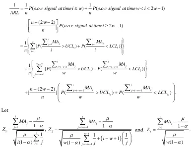
Proof. The proposition I and II can be analytically derived by central limit theorem as follows. The average run length values can be derived. LetARLn,then

1 1 1

( . . ) ( . . 2 1)

 P o o c signal at timeiw  P o o c signal at time w i w

ARL n n

(2 w 2)

( . . 2 1)

 

_ _  

 

n

P o o c signal at time i w

n 1 1 1 1 [ (  ) (  )]   _    _    



i i w j j j j i i i MA MA

P UCL P LCL

n i i

2 2 1 1 1 1 [ ( ) ( )]            _    _    



i i w j j

j i w j i w

i i

j i w

MA MA

P UCL P LCL

n w w

1 1 (2 2) [ ] ( ) ( ) . i i j j

j i w j i w

w w

MA MA

n w

P UCL P LCL

n w w

                 



Let 1 1 1 1 1 (1 )

,

         



i j j i j MA Z

i j





1 2 1 1 1 1 1 1 (1 )                        



i j j i w

w

j i w

MA

Z

i w

w j j

and 3 1

1 (1 ) .         



i j j MA Z w 3. Results

The numerical results for ARL0 and ADT of DMA chart are calculated from Equation (4) and Equation (5). The parameter values for DMA chart following moving average considering w= 2, 3, 4, 5, 10 and 15. The in-control parameter are given ₀= 1, 3 and ₀= 0.2. Out-of-control parameter values are 1 and shift parameters (



1) = 0.1, 0.2, 0.3,…, 2.0. Out-of-control parameter values are 1 and shift parameters (



₂) = 0.1, 0.2, 0.3,…, 2.0. Out-of-control parameter values are



1/ 1



1 and

shift parameters (



) = 0.1, 0.2, 0.3,…, 2.0. The results show that the proposed DMA chart are sensitive to only a few of the out-of-control situations.

Table I shows ARL for 0= 1 of DMA chart considering a change in , when small shifts (δ ≤ 0.5), the DMA chart has the best performance with w = 15. For moderate shifts (0.6 ≤ δ ≤ 0.8) the performance of DMA chart with w= 10 is superior to others. For the shift sizes (0.9 ≤ δ ≤ 1.0) the performance of DMA chart with w= 5 is the best control chart. For large shifts (δ > 1.5), the DMA chart has the best performance withw= 4. Table II shows the ARL for ₀ = 3 of DMA chart considering a change in , when small shifts (δ ≤ 0.3) the DMA chart has the best performance with

(7)

Table 1. ARL of DMA chart for given ₀= 1, ₀= 0.2and considering a change in .

1



_w_{= 2} w = 3 w = 4 w = 5 w = 10 w = 15

0.0 370.398 370.398 370.398 370.398 370.398 370.398

0.1 201.525 173.237 144.981 119.819 52.267 37.871*

0.2 101.168 70.595 49.631 36.400 20.347* 25.745

0.3 53.518 32.788 21.917 16.632 16.182* 22.985

0.4 30.909 17.946 12.51 10.627* 14.537 19.277

0.5 19.475 11.361 8.696 8.296* 12.952 15.033

0.6 13.253 8.086 6.879* 7.160 11.161 11.468

0.7 9.629 6.290 5.883* 6.468 9.375 8.942

0.8 7.389 5.219* 5.261 5.956 7.824 7.273

0.9 5.933 4.530* 4.824 5.519 6.593 6.163

1.0 4.943 4.057* 4.482 5.116 5.655 5.382

1.5 2.816* 2.894 3.272 3.443 3.355 3.347

2.0 2.126* 2.307 2.450 2.461 2.434 2.434 * is minimum ADT.

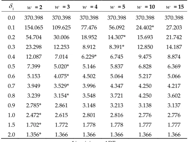
Table 2. ARL of DMA chart for given ₀= 3, ₀= 0.2and considering a change in .

1



_w_{= 2} w = 3 w = 4 w = 5 w = 10 w = 15

0.0 370.398 370.398 370.398 370.398 370.398 370.398

0.1 154.065 109.625 77.476 56.092 24.402* 27.203

0.2 54.704 30.006 18.952 14.307* 15.693 21.742

0.3 23.298 12.253 8.912 8.391* 12.850 14.187

0.4 12.087 7.014 6.229* 6.745 9.475 8.874

0.5 7.399 5.020* 5.146 5.837 6.828 6.369

0.6 5.153 4.075* 4.502 5.064 5.217 5.066

0.7 3.949 3.529* 3.996 4.347 4.250 4.217

0.8 3.239 3.154* 3.548 3.721 4.250 3.602

0.9 2.785* 2.861 3.148 3.213 3.138 3.137

1.0 2.472* 2.615 2.801 2.816 2.776 2.776

1.5 1.702* 1.772 1.778 1.778 1.777 1.777

2.0 1.356* 1.366 1.366 1.366 1.366 1.366 * is minimum ADT.

(8)

4. For parameter shifts (δ ≤ 1.5), the DMA chart has good performance with w= 3. For parameter shifts (δ ≤ 2.0), the DMA chart has good performance with w= 2.

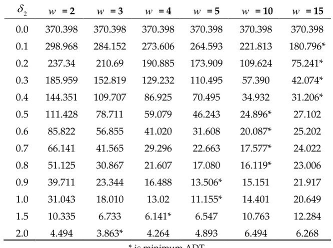
Table 3. ARL of DMA chart for given ₀= 1, ₀= 0.2and considering a change in .

2



_w_{= 2} _w_{= 3} _w_{= 4} _w_{= 5} _w_{= 10} _w_{= 15}

0.0 370.398 370.398 370.398 370.398 370.398 370.398

0.1 298.968 284.152 273.606 264.593 221.813 180.796*

0.2 237.34 210.69 190.885 173.909 109.624 75.241*

0.3 185.959 152.819 129.232 110.495 57.390 42.074*

0.4 144.351 109.707 86.925 70.495 34.932 31.206*

0.5 111.428 78.711 59.079 46.243 24.896* 27.102

0.6 85.822 56.855 41.020 31.608 20.087* 25.202

0.7 66.141 41.565 29.296 22.663 17.577* 24.022

0.8 51.125 30.867 21.607 17.080 16.119* 23.006

0.9 39.711 23.344 16.488 13.506* 15.151 21.917

1.0 31.043 18.010 13.02 11.155* 14.401 20.649

1.5 10.335 6.733 6.141* 6.547 10.763 12.284

2.0 4.494 3.863* 4.264 4.893 6.494 6.268 * is minimum ADT.

Table 4. ARL of DMA chart for given ₀3,00.2 and considering a change in .

2



_w_{= 2} w = 3 w = 4 w = 5 w = 10 w = 15

0.0 370.398 370.398 370.398 370.398 370.398 370.398

0.1 291.784 270.623 252.542 235.367 158.437 108.104*

0.2 217.048 178.177 147.713 122.847 56.437 40.275*

0.3 155.32 111.86 83.083 63.430 28.700 28.590*

0.4 108.909 69.874 48.025 35.266 20.289* 25.573

0.5 75.922 44.520 29.402 21.751 17.190* 24.007

0.6 53.155 29.316 19.305 14.952* 15.698 22.378

0.7 37.625 20.09 13.635 11.330* 14.673 20.276

0.8 27.043 14.375 10.322 9.276* 13.707 17.730

0.9 19.794 10.748 8.300 8.028* 12.644 15.033

1.0 14.783 9.385 7.010* 7.207 11.447 12.510

1.5 4.772 3.944* 4.362 4.963 5.729 5.438

2.0 2.479* 2.638 2.935 3.071 3.032 3.018 * is minimum ADT.

(9)

/1

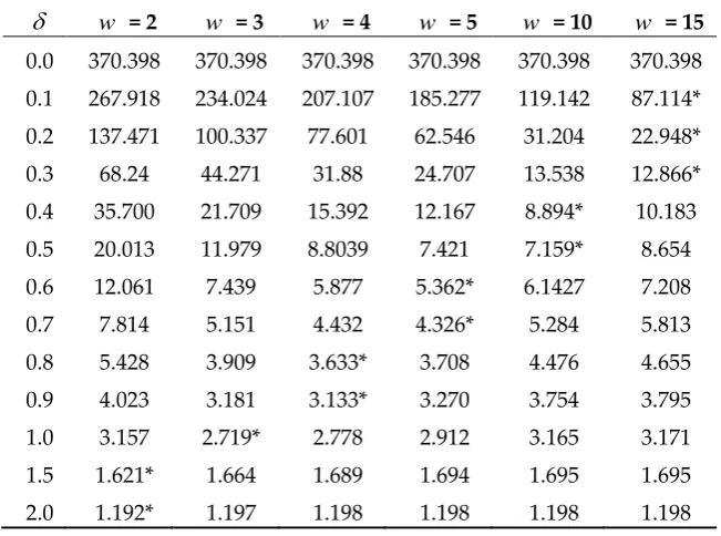
 , when small shifts (δ ≤ 0.3), the DMA chart has the best performance with w= 15. For moderate shifts (0.4 ≤ δ ≤ 0.5), the DMA chart has good performance with w= 10. For magnitude of shifts (0.6 ≤ δ ≤ 0.7), the DMA chart has good performance with w = 5. For parameter shift (0.8 ≤ δ ≤ 0.9), the DMA chart has the performance with w= 4. For parameter shifts (δ ≤ 1.0), the DMA chart has good performance with w= 3. For parameter shifts (1.5 ≤ δ ≤ 2.0), the DMA chart has good performance with w= 2.

The average run length for DMA chart shows that when the shift increases, the DMA performs better when the value of (w) decreases. Therefore, one can see that the proposed formulas for ARL0 and ADT for DMA chart can correctly calculate efficiently. Moreover, this is easy to implement which should also greatly reduce computation times.

Table 5. ARL of DMA chart for given ₀= 1, ₀= 0.2and considering a change in / 1







.



w = 2 w = 3 w = 4 w = 5 w = 10 w = 15 0.0 370.398 370.398 370.398 370.398 370.398 370.398

0.1 329.399 311.906 296.057 281.64 225.731 187.864*

0.2 244.313 206.88 178.542 156.438 94.298 67.119*

0.3 166.124 126.463 100.728 82.916 42.669 30.139*

0.4 110.348 77.170 58.018 45.897 22.805 17.995*

0.5 73.723 48.334 34.988 27.154 14.518 13.397*

0.6 50.111 31.352 22.263 17.293 10.722* 11.312

0.7 34.805 21.130 14.989 11.872 8.7909* 10.111

0.8 24.743 14.816 10.682 8.756 7.677* 9.206

0.9 18.017 10.811 8.041 6.883* 6.931 8.372

1.0 13.441 8.204 6.363 5.704* 6.349 7.538

1.5 4.424 3.389 3.282* 3.407 3.986 4.057

2.0 2.377 2.263* 2.359 2.439 2.506 2.506 * is minimum ADT.

Table 6. ARL of DMA chart for given ₀= 3, ₀= 0.2and considering a change in / 1







.



w = 2 w = 3 w = 4 w = 5 w = 10 w = 15 0.0 370.398 370.398 370.398 370.398 370.398 370.398

0.1 267.918 234.024 207.107 185.277 119.142 87.114*

0.2 137.471 100.337 77.601 62.546 31.204 22.948*

0.3 68.24 44.271 31.88 24.707 13.538 12.866*

0.4 35.700 21.709 15.392 12.167 8.894* 10.183

0.5 20.013 11.979 8.8039 7.421 7.159* 8.654

0.6 12.061 7.439 5.877 5.362* 6.1427 7.208

0.7 7.814 5.151 4.432 4.326* 5.284 5.813

0.8 5.428 3.909 3.633* 3.708 4.476 4.655

0.9 4.023 3.181 3.133* 3.270 3.754 3.795

1.0 3.157 2.719* 2.778 2.912 3.165 3.171

1.5 1.621* 1.664 1.689 1.694 1.695 1.695

(10)

4. Discussion

The best properties of a DMA chart are memory control charts because of their ability to detect small shifts. Without loss of generality, this chart can be relaxed due to its feasibility with the width of control limit (w). The DMA chart performs better as the values of wincreases for small shifts, however, the number of observations must be sufficiently large.

5. Conclusions

The explicit formulas for ARL of DMA for Poisson counting process was derived. The INAR(1) model is a simple but well interpretable model for correlated process of Poisson counts data. The result shows that when a process increases, the performance of DMA will perform better as the value of w_{decreases for all case studies. Furthermore, these explicit formulas are simple and easy to}

implement which reduces computation time to less than 1 second.

Acknowledgments: This research is granted from National Research Council of Thailand with contract no. KMUTNB-GOV-60-XX. The author would like to express gratitude to the Graduate Collage of King Mongkut’s University of Technology, North Bangkok, Thailand. Also thanks to the Department of Applied Statistics for supporting materials and high performance computer.

Conflicts of Interest: The authors declare no conflict of interest.

References

1. Harris, T.E. 1963. The Theory of Branching Processes, Springer, Berlin, 1963.

2. Weiβ, C.H. Controlling correlated processes of Poisson counts. Quality Reliability Engineering International 2007, 23, 741-754.

3. Montgomery, D.C. Statistical Quality Control, 6th ed.; John Wiley & Sons, New York, 2009.

4. Roberts, S.W. Control chart tests based on geometric moving average. Technometrics 1959, 1, 239-250. 5. Page, E.S. Continuous inspection schemes. Biometrika 1954, 41, 100-144.

6. Khoo, M.B.C. A moving average control chart for monitoring the fraction non-conforming. Journal of Quality and Reliability Engineering International 2004, 20, 617-635.

7. Khoo, M.B.C; Wong, V.H. A double moving average control chart. Communications in Statistics-Simulation and Computation 2008, 37, 1696-1708.

8. Brockwell, P.J.; Davis, R.A. Time Series: Data Analysis and theory, 2nd ed.; Springer, New York, 2009. 9. McKenzie, E. Some simple models for discrete variate time series. Water Resources Bulletin 1985, 21, 645-650. 10. Al.Osh, M.A.; Alzaid, A.A. First-order integer-valued autoregressive (INAR(1)) process. Journal of Time

Series Analysis 1987, 8, 261-275.

11. McKenzie, E. Discrete Variate Time Series in Handbook of statistics eds, Shanbhag, D.N., Rao, C.R., Elsevier Amsterdam, 2003; volume 20, pp. 573-606.

12. Crowder, S.V. A simple method for studying run length distributions of exponentially weighted moving average charts. Technometrics 1979, 29, 401-407.

13. Brook, D.; Evans, D.A. An approach to the probability distribution of Cusum run length. Biometrika 1972, 9, 539-548.

14. Areepong, Y.; Novikov, A.A. Martingale approach to EWMA control chart for changes in Exponential distribution. Journal of Quality Measurement and Analysis 2008, 4, 197-203.

15. Areepong, Y.; Sukparungsee, S. An analytical ARL of binomial double moving average chart. International Journal of Pure and Applied Mathematics 2011, 73, 477-488.

16. Areepong, Y. Explicit formulas of Average Run Length for a Moving Average control chart for monitoring the number of defective products. International Journal of Pure and Applied Mathematics 2012, 80, 331-343. 17. Areepong, Y.; Sukparungsee, S. Closed form formulas of average run length of moving average control

chart for nonconforming for zero-inflated process. Far East Journal of Mathematical Sciences 2013, 75, 385-400. 18. Sukparungsee, S. Average run length of double moving average control chart for zero-inflated count

processes. Far East Journal of Mathematical Sciences 2013, 1, 85-103.

(11)

20. Phantu, S.; Sukparungsee, S.; Areepong, Y. Explicit expressions of average run length of moving average control chart for poisson integer valued autoregressive model. Lecture Notes in Engineering and Computer Science 2016, 2, 892-895.

21. Steutel, F.W.; Harn, K.V. Discrete analogues of self decomposability and stability. Annals of Probability 1979, 7, 839-899.