It is recommended that you read all instructions below; even if you are familiar with online
review practices.
Using the Smart Proof system, proof reviewers can easily review the PDF proof, annotate
corrections, respond to queries directly from the locally saved PDF proof, all of which are
automatically submitted directly to
our database
without having to upload the annotated PDF.
Before
completing your review...
Did you reply to all author queries found in your proof?
Did you click the "Publish Comments" button to save all your corrections?
Any unpublished comments will be lost.
Note:
Once you click "Complete Proof Review" you will not be able to add or
publish additional corrections.
L
o
gin into
Smart Proof
anywhere you are connected to the
internet.
Review the proof
on the following pages and mark corrections,
changes, and query responses using the
Annotation Tools
.
Note:
Editing
done by replacing the text on this
PDF is not
permitted with this application.
Save your proof corrections
by clicking the "Publish Comments"
button.
Corrections don't have to be marked in one sitting. You can
publish comments and log back in at a later time to add and
publish more comments before you click the "Complete Proof
Review" button below.
Complete your review
after all corrections have been published
to the server by clicking the "Complete Proof Review" button
below.
Publish Comments
Adding Comments and Notes to Your PDF
To facilitate electronic transmittal of corrections, we encourage authors to utilize the
comment/annotations features in Adobe Acrobat. The PDF provided has been
comment
enabled,
which allows you to utilize the comment and annotation features even if using
only the free Adobe Acrobat reader (see note below regarding acceptable versions).
Adobe Acrobat’s Help menu provides additional details on the tools. When you open
your PDF, the annotation tools are clearly shown on the tool bar (although icons may
differ slightly among versions from what is shown below).
For purposes of correcting the PDF proof of your journal article, the important features to
know are the following:
x
To
insert text,
place your cursor at a point in text and select the Insert Text tool (
)
from the menu bar. Type your additional text in the pop-up box.
x
To
replace text,
highlight the text to be changed, select the Replace Text tool (
) from
the menu bar, and type the new text in the pop-up box. Do this instead of deleting and then
reinserting.
x
To
delete text,
highlight the text to be deleted and press the Delete button on the
keyboard.
x
Use the
Sticky Note tool
(
) to describe changes that need to be made (e.g., changes
in bold, italics, or capitalization use; altering or replacing a figure) or to answer a
question or approve a change from the editor. To use this feature, click on the Sticky
Note tool in the menu bar and then click on a point in the PDF where you would like to
make a comment. Then type your comment in the pop-up box.
x
Use the
Callout tool
(
) to point directly to changes that need to be made. Try to put
the callout box in an area of white space so that you do not obscure the text.
x
Use the
Highlight and Add Note to Text tool
(
) to indicate font problems, bad
breaks, and other textual inconsistencies. Select text to be changed, choose this tool, and
type your comment in the pop-up box. One note can describe many changes.
changes clearly and thoroughly, to answer all queries and questions, and to provide
complete information to allow us to make the necessary changes to your article so it is
ready for publication. Do not use tools that incorporate changes to the text in such a way
that no indication of a change is visible. Such changes will not be incorporated into the
final proof.
To utilize the comments features on this PDF you will need Adobe Reader version
7 or higher. This program is freely available and can be downloaded from
5
For information about becoming a member of the American Psychological Association, visit http://www.apa.org/membership/index.aspx; or call the Membership Office at 1-800-374-2721.
2019 APA Journal Subscription Rates
---
Instructions: Check the appropriate box, enter journal title and price information, and complete the mailing label in the right column. Enclose a check made out to the American Psychological Association, and mail it with the form to the APA Order Department or complete the credit card information below. Orders can also be placed online at http://www.apa.org/pubs/journals/subscriptions.aspx.
Annual Subscription (available on January-December basis only). Refer to the Subscription Rates shown above.
Journal: _____________________________________________
Price: ________________________
Special Offers! If you are a journal article author, you may take advantage of two Special Offers.
Individual Copy. You may order individual copies of the entire issue in which your article appears. As an author, you receive a special reduced rate of $5 per copy for up to a maximum of 25 copies. No phone requests accepted.
Journal: ____________________________________________
Vol. no.: _______ Issue no.: _______ Issue month: _________
____ copies @ $5 a copy = $________ (order amount) +________ (handling; see below) TOTAL enclosed: $________
Shipping & Handling Fees
Order amount: U.S. & Puerto Rico Guaranteed Non-U.S.*
Economy Non-U.S.**
Up to $14.99 $5.00 $50.00 $15.00
$15 to $59.99 $6.00 $75.00 $16.00
$60.00+ 10% Order Total $125.00 $20.00
*International rates for guaranteed service are estimates.
**I agree that international economy service is non-guaranteed and does not provide tracking or date/time specific delivery. Delivery time for this level of service can take up to 8 weeks. If this level of service is selected, APA will not
be held liable and will not honor any claims for undelivered, delayed, or lost shipments.
Hardship Request. If you do not have a personal subscription to the journal and you do not have access to an institutional or departmental subscription copy, you may obtain a single copy of the issue in which your article appears at no cost by filing out the information below.
Journal: ___________________________________________ Vol. no. : _________________ Issue no.: _________________ Issue month: ________________________________________
CREDIT CARD PAYMENT
___ VISA ___ MASTERCARD ___ AMERICAN EXPRESS CARD NUMBER__________________________________________ Expire Date ___________ Signature __________________________
PRINT CLEARLY – THIS IS YOUR MAILING LABEL
Send the completed form and your check, made out to the American Psychological Association, or your credit card information to:
APA Order Department 750 First Street, NE Washington, DC 20002-4242
All orders must be prepaid. Allow 4-6 weeks after the journal is published for delivery of a single copy or the first copy of a
subscription.
SHIP TO: Phone No. ____________________
Name _______________________________________ Address ______________________________________ _____________________________________________ City ________________ State ________ Zip ________
Expedited Service (enter service required): ___________
Journal*
Non-Agent Individual
Rate
APA Member
Rate Journal*
Non-Agent Individual
Rate
APA Member
Rate
American Psychologist $ 472 $ 12 Jrnl of Family Psychology $ 271 $ 131
Behavioral Neuroscience $ 488 $ 200 Jrnl of Personality & Social Psychology $ 831 $ 297
Developmental Psychology $ 595 $ 212 Neuropsychology $ 271 $ 131
Emotion $ 204 $ 131 Professional Psych: Research & Practice $ 223 $ 71
Experimental & Clinical Psychopharmacology $ 150 $ 103 Psychological Assessment $ 328 $ 175
History of Psychology $ 151 $ 82 Psychological Bulletin $ 328 $ 175
Jrnl of Abnormal Psychology $ 282 $ 131 Psychological Methods $ 211 $ 98
Jrnl of Applied Psychology $ 562 $ 175 Psychological Review $ 271 $ 113
Jrnl of Comparative Psychology $ 164 $ 71 Psychology & Aging $ 271 $ 131
Jrnl of Consulting & Clinical Psychology $ 406 $ 175 Psychology of Addictive Behaviors $ 271 $ 131
Jrnl of Counseling Psychology $ 223 $ 98 Psychology, Public Policy, and Law $ 164 $ 71
Jrnl of Educational Psychology $ 271 $ 131 Rehabilitation Psychology $ 164 $ 71
JEP: Animal Learning and Cognition $ 164 $ 71 Clinician’s Research Digest – Adult $ 164 $ 71
JEP: Applied $ 164 $ 71 Populations
JEP: General $ 445 $ 175 Clinician’s Research Digest – Child and $ 164 $ 71
JEP: Human Perception, and Performance $ 562 $ 212 Adolescent Populations
JEP: Learning, Memory, and Cognition $ 562 $ 212
An Advantage for Smooth Compared With Angular Contours in the Speed
of Processing Shape
Marco
Bertamini
University of Liverpool and University of Padova
Letizia
Palumbo
Liverpool Hope University
Christoph
Redies
Friedrich Schiller University of Jena
Curvature along a contour is important for shape perception, and a special role may be played by points of maxima (extrema) along the contour. Angles are discontinuities in curvature, a special case at one extreme of the curvature continuum. We report 4 studies using abstract shapes and comparing polygons (curvature discontinuities at the vertices) and a smoothed version of polygons (no vertices). Polygons are simpler and are defined by a small set of vertices, whereas smoothed shapes have a continuous curvature change along the contour. Angles have also been discussed as an early signal of threat and danger, and on that basis, one may predict faster responses to polygons. However, curved shapes are more typical of the natural environment in which the visual system has evolved. For a detection task, we found faster responses to smooth shapes, not mediated by complexity (Experiment 1). We then tested 3 orthogonal shape tasks: comparison between shapes (detection of repetition; Experiment 2a), comparison after a rotation (Experiment 2b), and detection of bilateral symmetry (Experiment 3). In all tasks, responses for smoothed stimuli were faster; there was also an interaction with type of response: Trials with smooth shapes were faster when a positive response was produced. Overall, there was evidence that smooth shapes with continuous change in curvature along the contour are processed more efficiently, and they tend to be classified as targets. We discuss this in relation to shape analysis and to the preference for smoothed over angular shapes.
Public Significance Statement
The study demonstrates that shapes with smooth curvature are processed more quickly and efficiently compared with shapes with sharp angles. This perceptual factor may clarify the link between perception and preference because smooth shapes are known to be preferred.
Keywords:perception, visual preference, curvature, complexity
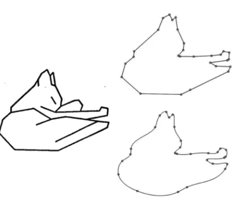
In his seminal article,Attneave (1954)noted that, along con-tours, points of maximal curvature carry the greatest information. He designed a now-famous example using an image of a cat, reproduced inFigure 1. He selected 38 points of maximal curva-ture from the boundary contour of the image of a sleeping cat and connected them with lines. For most people, the cat is still easy to
recognize. In a second demonstration, Attneave asked people to mark salient points along the contour of a random shape. Here, too, the points selected were close to the locations of maximal curva-ture. These locations with peaks of curvature (curvature extrema) are the sharp turns along the contour. The idea is that they allow the extraction of an economical description of objects.
The importance of curvature extrema has been studied and confirmed by empirical studies.De Winter and Wagemans (2008) found that participants were most likely to pick up local curvature maxima when asked to mark salient points along the contour line of 2-D shapes (see also Norman, Phillips, & Ross, 2001). An explicit representation of curvature has also been implemented within formal models of vision (Asada & Brady, 1984). In general, a role for curvature extrema is acknowledged in theories of shape representation (Cohen & Singh, 2007;De Winter & Wagemans, 2006,2008;Feldman & Singh, 2005;Hoffman & Richards, 1984; Hoffman & Singh, 1997;Leyton, 1989). There is also evidence that attention is allocated preferentially to regions near corners (Bertamini, Helmy, & Bates, 2013; Cole, Skarratt, & Gellatly,
X Marco Bertamini, Department of Psychological Sciences, University of Liverpool, and Department of General Psychology, University of Pa-dova; Letizia Palumbo, Department of Psychology, Liverpool Hope Uni-versity; Christoph Redies, Institute of Anatomy, Jena University Hospital, Friedrich Schiller University of Jena.
This work was supported in part by the Economic and Social Research Council (ESRC, Ref. ES/K000187/1).
Correspondence concerning this article should be addressed to Marco Bertamini, Department of Psychological Sciences, University of Liverpool, Eleanor Rathbone Building, Bedford Street South, L69 7ZA, Liverpool, United Kingdom. E-mail:[email protected]
This
document
is
copyrighted
by
the
American
Psychological
Association
or
one
of
its
allied
publishers.
This
article
is
intended
solely
for
the
personal
use
of
the
individual
user
and
is
not
to
be
disseminated
broadly.
Journal of Experimental Psychology:
Human Perception and Performance
© 2019 American Psychological Association 2019, Vol. 1, No. 999, 000
0096-1523/19/$12.00 http://dx.doi.org/10.1037/xhp0000669
1
AQ: au AQ: 1
AQ: 2
AQ: 3
AQ: 4
F1
AQ: 5
2007), perhaps due to the fact that these are more informative locations. Many studies have also highlighted how positive and negative extrema (convexities and concavities) carry information about solid shape (Bertamini & Wagemans, 2013; Hoffman & Richards, 1984;Koenderink, 1984).
Separately from the literature on curvature extrema, there is evidence from experimental aesthetics that smooth curvature along contours or surfaces is preferred to angular contours (Bar & Neta, 2006;Bertamini, Palumbo, Gheorghes, & Galatsidas, 2016;Silvia & Barona, 2009). We review this literature next and then consider a possible link with perception. To fill a gap in the empirical studies, we conducted four experiments to compare angular and smooth versions of abstract shapes on three different perceptual tasks. Byangular2-D shapes, we mean irregular polygons. These have sharp angles that are easy to see and locate. Bysmooth2-D shapes, we mean similar polygons (generated by the same algo-rithm) that have been converted into shapes with a continuously changing curvature along the contour. We carefully controlled that the same series of convexities and concavities were present in both sets. To anticipate the results, despite the fact that angular shapes are simpler, we found an advantage in processing smooth shapes on perceptual tasks, and we speculate that this may be a contrib-uting factor to their preference.
Preference for Smooth Curvature
Shapes with smooth curvature along their contours are preferred to shapes with more angular contours, as observed by both artists and psychologists (for the historical background, seeBertamini & Palumbo, 2015; Gómez-Puerto, Munar, & Nadal, 2016). This phenomenon is true for both familiar objects and abstract shapes (Bar & Neta, 2006;Bertamini et al., 2016;Silvia & Barona, 2009), it has been confirmed in different cultures (Gómez-Puerto et al.,
2018) in children (Jadva, Hines, & Golombok, 2010) and in other species such as great apes (Munar, Gómez-Puerto, Call, & Nadal, 2015), and it has been measured also using implicit tasks of preference or approach (Palumbo & Bertamini, 2016; Palumbo, Ruta, & Bertamini, 2015).
The relationship between perception, including attention alloca-tion, and preference is fascinating but complex. If corners are important for shape analysis and attract attention, and if one assumes that stimuli that are salient for perception are also liked more, one could formulate the prediction of a preference for angularity. The same conclusion may be based on a differential in processing speed, which may affect preference through a process of fluency (Reber, Winkielman, & Schwartz, 1998). However, this is the opposite of what the empirical studies have consistently found: Smooth shapes are preferred to angular shapes.Bar and Neta (2007)have suggested that this is due to the role of angles in threat detection. Supporting this hypothesis, they found that the amygdala, a structure involved in fear processing, is significantly more active for angular objects compared with similar but less angular objects. Recently, Grebenkina, Brachmann, Bertamini, Kaduhm, and Redies (2018)found that edge-orientation entropy predicted aesthetic ratings. This factor shares a large portion of predicted variance with the preference for curved over angular stimuli.
The difference in preference between angular and smooth shapes was the original motivation for the current set of studies. Given that the preference for smooth curvature is a robust effect, we need to know more about how shapes with smooth curvature along their contours are perceived.
Reasons to Expect Faster Responses to Angular or to
Smooth Shapes
We set out to explore the difference between shapes with angular and smooth contours for different perceptual tasks. A case can be made to expect faster responses to shapes with angular contours, but an alternative case can be made to expect faster responses to shapes with smooth contours.
One hypothesis is that angular shapes, because of their relative simplicity, because of the salience of angles (Bertamini et al., 2013;Cole et al., 2007), or because of the threat association (Bar & Neta, 2006;Larson, Aronoff, Sarinopoulos, & Zhu, 2009; Lar-son, Aronoff, & Stearns, 2007), will generally lead to faster responses. The opposite is also possible. Small changes in orien-tation may facilitate contour integration (Bex, Simmers, & Dakin, 2001;Field, Hayes, & Hess, 1993). A smooth contour is a contour in which, at any point, change of orientation is small compared with the abrupt change for an angular shape; therefore, contour integration is more efficient for smooth contours. Neurophysiolog-ical evidence supports a role for curvature in how shape is encoded in early visual areas, in particular in V4 (Pasupathy & Connor, 2002), and explicit coding of local curvature is implied by the presence of curvature aftereffects (Gheorghiu & Kingdom, 2007, 2008;Suzuki & Cavanagh, 1998).
These two hypotheses are extreme scenarios. It is important to compare different tasks because advantages and disadvantages may vary depending on the task; for example, contour integration may be relevant only when global shape has to be extracted and analyzed. Finally, for tasks in which there is a correct and an Figure 1. The image on the left shows a reproduction of the original
demonstration byAttneave (1954)with 38 vertices. The original photo-graph of a cat is not available. The polygon (top right) is based on 28 vertices around the outside of the image, and the last image is a version of the same shape with smooth contours. Without information inside the shape, it is hard to recognize the cat, but angular and smooth versions have similar overall information.
This
document
is
copyrighted
by
the
American
Psychological
Association
or
one
of
its
allied
publishers.
This
article
is
intended
solely
for
the
personal
use
of
the
individual
user
and
is
not
to
be
disseminated
broadly.
AQ: 6
AQ: 7
incorrect answer, there can also be differences in criterion, with observers more willing to provide a positive response to some shapes than others. For example,Brodeur, Chauret, Dion-Lessard, and Lepage (2011)reported that in a memory task, there was a bias to classify symmetrical shapes as familiar. This was not a differ-ence in sensitivity but in response bias.
Summary of Experiments
In Experiment 1, we used a simple task in which observers had to respond to the shapes on the basis of whether they belonged to one or the other of the two categories. In this task, observers had to press a key as soon as a stimulus appeared on screen when it was angular (in one set of trials) or when it was curved (in a different set of trials). This can therefore be described as a variation on the inhibition control procedure (Logan & Cowan, 1984). We used abstract shapes that were either angular (polygons) or curved (smoothed version of polygons) and varied in complexity. The aim was to test whether angular shapes produce faster responses than smoothly curved shapes.
For Experiment 2, we wanted a task in which the whole shape had to be processed. We presented two shapes side by side and the task was to judge whether they were the same. They could be either both angular or both curved (never a mix of the two). The aim was to test processing of global shape while the angularity of the stimuli was not task relevant. In Experiment 2a, the shapes were presented side by side; in Experiment 2b, the task was harder because one shape was rotated by 180°.
The aim for Experiment 3 was to test the role of shape in a symmetry detection task. As in Experiment 2, the task required processing of the whole shape. The comparison in this case was between two contours, which could match (bilateral symmetry) or be different and unrelated (asymmetrical). The information about whether the contours were angular or smoothly curved was not relevant for the task.
For both Experiments 2 and 3, the study was designed to record and analyze speed of responses and errors. In a separate analysis, we measured sensitivity and response bias using a signal detection approach. However, the task was easy because we wanted to minimize errors, and therefore we are aware that, given the focus on response time, we are likely to see a ceiling effect in terms of correct responses.
To estimate the expected effect size, we looked at a study in which the observer was presented with simple polygons and the task was to discriminate between two different shapes (Bertamini & Farrant, 2006). The dependent variable was response time and the average effect size over the three experiments was 0.28 (p2) and therefore 0.62 (Cohen’s f). We used GⴱPower (Version 3.1.9; Faul, Erdfelder, Buchner, & Lang, 2009) and entered this effect size, an alpha of 0.05, and a power of 0.95. For a main effect in an ANOVA with repeated measures, the necessary sample size was 11. We decided on a more conservative sample size of 26 and also made an explicit decision that this sample size would be kept the same across all our experiments.
Experiment 1: Detection Response Time
There were two parts in this experiment. During the first part, the observer produced a response (pressing the space bar) when an
angular shape was shown on the screen, and waited without responding when a smooth shape was shown on the screen. In another set of trials, the observer produced a response when a smooth shape was shown, and waited without responding when an angular shape was shown. If no response was produced, the shape disappeared after 4 s. Every participant performed both types of tasks in a balanced design. The aim was to see whether observers are faster to produce a response to one or the other of the two types of shapes. The positive response to a specific type of stimulus was inspired in part by the existing techniques using response inhibi-tion (e.g., go/no-go task;Nosek & Banaji, 2001).
The stimuli were always unfamiliar abstract shapes, and no shape was ever repeated twice within a task. The color of the shape was lighter than the background or darker than the background (with equal probability). Therefore, in one case, the onset of the stimulus coincided with an increase in luminance, and in the second case, it coincided with a decrease in luminance.
To vary the complexity of the shapes, we varied the number of vertices. The polygon could have 10, 20, or 30 vertices. In addi-tion, we controlled number of convexities and concavities, as this is likely to affect perceived part structure (Bertamini & Wage-mans, 2013). Concavities could be 30%, 40%, or 50% of the total number of vertices. Therefore, for 10 vertices, concavities were 3, 4, or 5; for 20 vertices, they were 6, 8, or 10; and for 30 vertices, they were 9, 12, or 15.
Method
Participants. Twenty-six participants took part (Mage⫽24 years; two left-handed; 14 females). All participants had normal or corrected-to-normal vision. They provided a written consent for taking part and received course credits. The experiment was ap-proved by the Ethics Committee of the University of Liverpool and was conducted in accordance with the Declaration of Helsinki (2008).
Stimuli and apparatus. Stimuli were created using python and Psychopy (Peirce, 2007). The shapes were generated by sam-pling locations along a circle and connecting these locations to create a polygon. When sampling a location for a vertex, the radius (i.e., distance from the center) was not kept constant. Instead, it varied randomly between 110 and 210 pixels. Therefore, the polygon was irregular. The locations (sides of the polygon) were either 10, 20, or 30. Concave vertices were 30%, 40%, or 50% of the total number of vertices. The way that convex and concave vertices formed a sequence was not constrained, and therefore more than one convex or more than one concave vertex could follow each other, creating more complex convexities or concav-ities. Alternating convex and concave vertices would have created highly regular star patterns.
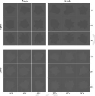
To create smooth stimuli, we started with a polygon and gen-erated a smoothed version by fitting a curve through the vertices using a cubic spline (see Bertamini et al., 2016, for a similar approach). The smoothed contour did pass through all the vertices of the original polygon. The difference between the curved and angular stimuli can be seen in Figure 2. Note that these are examples, because in every trial, we used a different set of vertices and, therefore, no shape was repeated twice during one session (i.e., one task). In other words, there were 252 different shapes.
This document is copyrighted by the American Psychological Association or one of its allied publishers. This article is intended solely for the personal use of the individual user and is not to be disseminated broadly.
3
CURVATURE AND SHAPE PROCESSING
AQ: 9 AQ: 10
AQ: 11
F2
Approximate size (max diameter) was 8 cm. The stimuli are available fromhttps://osf.io/4278q/.
The background was a uniform gray (approximate luminance⫽ 59 cd/m2). The color of the shape could be either lighter than the background (68 cd/m2) or darker than the background (53 cd/m2). This factor is called Color, and it implies that the onset could be an increase or a decrease of luminance.
Participants sat at approximately 60 cm from the screen. Stimuli were presented on a 1,280⫻1,024 pixelx Apple StudioDisplay 21-in. CRT monitor at 60 Hz.
Experimental design and procedure. A 2⫻2⫻3⫻2⫻2 design was employed. The within-subjects factors were Task (an-gular, curved), Shape (an(an-gular, curved), Color (light, dark), Com-plexity (10, 20, 30), and Concavity (30%, 40%, 50%). The only between-subjects factor was the order of the tasks, whether they responded to angular first or to curved first. The experiment lasted approximately 40 min.
The experiment began with the instructions followed by the practice session (18 trials). Each trial started with a fixation cross at the center of a gray background. This fixation lasted randomly between 500 and 1,500 ms. After that, the shape appeared and remained on screen until response. The response was entered with the space bar on a computer keyboard. Responses had to be entered within 4,000 ms of stimulus onset; otherwise, the trial would end and the program would move on to the next trial. In total, there
were 504 experimental trials, divided in two sessions with 252 trials for each of the two tasks.
Analysis. A mixed ANOVA was performed with Shape (an-gular, curved), Color (light, dark), Complexity (10, 20, 30), and Concavity (30%, 40%, 50%) as within-subjects factors, and Order (angular first, curved first) as between-subjects factor.
The dependent variable was the response time. We inspected the distribution, which was limited at one end by the 4,000-ms max-imum time for a response. In terms of wrong responses, there are two possible errors. First, participants pressed the space bar when they should not have done so. Second, participants did not press the space bar when they should have done so (and, therefore, time reached 4,000 ms). Errors were rare, and all errors (2.5% of trials in total) were removed. The analysis was carried out on the trials on which subjects were required to produce a response. In addi-tion, responses below 250 ms were removed because they were likely to be anticipation errors. They were extremely rare (0.05% of trials). Over all of the remaining trials, the mean response time was 692 ms and the standard deviation was 363 ms.
Results and Discussion
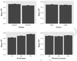
The response time results are illustrated in Figure 3. The ANOVA confirmed a main effect of shape,F(1, 24)⫽5.08,p⫽ .034,p2⫽0.17, with faster responses to smooth shapes; a main Figure 2. Experiment 1: Examples of angular stimuli (left) and smooth contour stimuli (right). Stimuli could
be darker than the background (top) or lighter (bottom). The three rows show the three levels of number of vertices: 10, 20, or 30. The three columns show the three levels of percentage of concave vertices.
This
document
is
copyrighted
by
the
American
Psychological
Association
or
one
of
its
allied
publishers.
This
article
is
intended
solely
for
the
personal
use
of
the
individual
user
and
is
not
to
be
disseminated
broadly.
effect of complexity,F(2, 48)⫽23.89,p⬍.001,p2⫽0.50, with responses becoming slower as complexity increased; a main effect of color, F(1, 24)⫽4.37,p⫽.047,p2⫽0.15, with responses faster when the shapes were lighter than the background; and a main effect of concavity,F(2, 48)⫽5.87,p⫽.005,p2⫽0.20, due to slower responses for the stimuli with 50% concave vertices. In terms of interactions, there was an interaction between color and order,F(1, 24)⫽4.98,p⫽.035,p2⫽0.17, and a three-way interaction between color, order, and complexity,F(2, 48)⫽3.71, p⫽.032,p2⫽0.13. It seems that there were faster responses to light stimuli when they were responded to first.
There were also some interactions involving shape, and inter-actions between shape, complexity, and concavity, F(4, 96) ⫽ 5.47, p ⬍ .001, p2 ⫽ 0.19, and between shape, complexity, concavity, and color, F(4, 96) ⫽ 4.09, p ⫽ .004, p2 ⫽ 0.15. Interpreting these effects required post hoc analyses. Because of its importance for our hypothesis, we conducted three separate tests of the effect of shape and complexity at each of the three levels of concavity. We wanted to see if the effect of these two key factors would be present in each subset of data. These were three repeated measures ANOVA, and we adjusted the alpha levels (from 0.05 to 0.008).
For 30% concave vertices, we confirmed the same effects of shape and complexity as in the main analysis. There was an effect of shape, F(1, 25) ⫽ 20.51, p⬍ .001, p2 ⫽ 0.45, with faster responses to smooth shapes; an effect of complexity,F(2, 50)⫽ 15.17,p⬍.001,p2 ⫽0.38, with responses becoming slower as complexity increased; and an interaction, F(2, 50) ⫽6.65, p⬍ .003, p2 ⫽ 0.21, in which, for angular stimuli, the slope was steeper as complexity increased.
For 40% concave vertices, there was an effect of shape,F(1, 25)⫽8.72,p⬍.007,p2⫽0.26, with faster responses to smooth
shapes, and an effect of complexity,F(2, 50)⫽21.57,p⬍.001,
p2 ⫽ 0.46, with responses becoming slower as complexity in-creased. By contrast, for 50% concave vertices, there was only a significant effect of complexity,F(2, 50)⫽14.01,p⬍.001,p2⫽ 0.36, with responses becoming slower as complexity increased.
These analyses show that constraining the amount of concavities can affect the comparison between angular and smooth stimuli. To understand this effect, it is useful to look at the stimuli inFigure 2: With many alternating convex and concave vertices, the smooth stimuli become very angular. Indeed, paradoxically, when a con-cave vertex is between two convex vertices and the distances are small, the curve has to turn very sharply to reach the vertex, creating a very pointy feature, one that may be sharper than when the vertices are connected by straight lines. In other words, some of the 50% concave stimuli may have been too complex and therefore degenerate to the point that angular and smooth versions would be hard to discriminate.
The method used to produce smooth contours starting from polygons implies that for smooth contours, the length of the contours will be slightly longer and the area slightly greater. On average, the length was 1,261 and the area was 78,057 for angular stimuli; for smooth stimuli, the length was 1,320 and the area was 78,802. These are pixels and squared-pixels values. As a percent-age, the smooth shapes were 4.4% longer and 0.9% larger than the angular shapes. To check the relationship between these parame-ters and response time, we looked at Pearson correlations over all trials. There was a correlation, as expected, between length and area ( ⫽0.468,p⬍.001) but no correlation between length and response time ( ⫽0.006,p⫽.503) or between area and response time ( ⫽0.001,p⫽.952).
Differences in contour length and complexity are not likely to explain the faster response to smooth shapes based on other Figure 3. Results of Experiment 1. Mean response time as a function of shape, color, complexity (number of
vertices), and concavity (percentage of concave vertices). Error bars are⫾1 SEM.
This
document
is
copyrighted
by
the
American
Psychological
Association
or
one
of
its
allied
publishers.
This
article
is
intended
solely
for
the
personal
use
of
the
individual
user
and
is
not
to
be
disseminated
broadly.
5
CURVATURE AND SHAPE PROCESSING
AQ: 33
AQ: 15
considerations as well. A much larger difference in contour length was present as a function of number of vertices. On average, the lengths were 1,102, 1,266, and 1,511 for 10, 20, and 30 vertices, respectively. This difference produced slower responses to the stimuli with longer perimeters, the opposite pattern when com-pared with the faster responses to smooth contours. We referred to the factor number of vertices ascomplexity. There is an interesting pattern, with slower responses to more complex stimuli (in terms of contour length and number of vertices) but faster responses to more complex stimuli (in terms of smooth change of orientation of the contour).1
Observers responded faster when they had to produce a response to smooth shapes. There were other factors, such as complexity and color, that influenced response time; however, the effect of shape did not interact with any other factor. The overall difference was of 50 ms in favor of the smooth contours. Speed of responses did not correlate with length of the contour; it did increase with complexity, as defined by number of vertices, whereas it decreased with smoothness. This apparent paradox may be understood in terms of the task. With an increase in number of vertices, angular and smooth stimuli become more similar because smooth stimuli become more and more pointy. Therefore, the discrimination task was harder and response time longer. Importantly, this phenome-non can explain the effect of number of vertices, but it cannot explain why responses were faster to smooth stimuli.
Post Hoc Analysis of Image Complexity
We have stated that smooth stimuli are more complex. There-fore, we decided to add an analysis of image complexity. We calculated two additional measures of objective image complexity for all stimuli. The first measure (termed gradient) is based on luminance gradient images that are used to calculate histograms of oriented gradients (Dalal & Triggs, 2005). The gradients are cal-culated using the MATLAB functiongradient. The mean of all gradient strengths in the gradient image is used as a measure of the objective complexity of each image. Low values indicate small changes in luminance gradients, and high mean values indicate large changes. For a detailed explanation of how this measure is calculated, see Braun, Amirshahi, Denzler, and Redies (2013, Appendix). The second measure is edge density and represents the sum of all Gabor filter responses in an image, using a bank of 24 oriented Gabor filters, as described in more detail in Redies, Brachmann, and Wagemans (2017). The higher the edge density, the more complex the image.
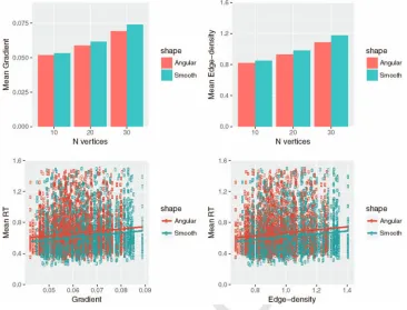
The graphs inFigure 4show mean values for the two objective complexity measures as a function of two different factors of Experiment 1 (number of vertices and shape), and the scatterplots show how complexity relates to reaction time. The total number of trials was 13,104, but because each observer only responded to one category at a time, we have response time for half of this total (n⫽ 6,552).
It is clear that both measures of complexity strongly depend on the number of vertices. In addition, independent of number of vertices, Figure 4 also shows that smooth stimuli were more complex than angular stimuli. The two scatterplots show that response time increases with objective complexity. This result is not surprising, as we had already seen that response time increases with number of vertices.
Next, we used a regression model to test the contribution of shape (angular vs. smooth) and objective complexity. As gradient and edge density were highly correlated for our stimuli ( ⫽0.99), we selected only one of them (gradient) for the regression. Gra-dient was centered by subtraction of the mean. We used linear mixed-effects models (lme4 package;Bates, Mächler, Bolker, & Walker, 2015) in R Version 3.3.3. The model included Shape and Gradient as factorial fixed effects. Participants was a random factor, and in addition, we included Number of Vertices as a second random factor. This is because the shapes with 10, 20, and 30 vertices are different types of objects, and response time varies with this factor. However, we are interested in evaluating the role of shape and complexity, and we are not interested at this stage in the role of number of vertices. The effects of the fixed predictors were tested via likelihood ratio (2) comparisons through the sequential decomposition of the model.
There was a significant negative effect of Shape ( ⫽ ⫺0.02),
2(1)⫽79.24,p⬍.001, but no significant effect of Gradient ( ⫽ 0.59), 2(1) ⫽ 3.10, p ⫽ .08, and no interaction ( ⫽ 0.28),
2(1)⫽1.34, p⫽.25. This mixed-effects model accounted for 0.9% of the variance without the random effect structure and 32.6% when it was included (R2m⫽ 0.009,R2c⫽0.326). This analysis confirms that the role of shape is a strong predictor of response time, even in comparison to objective measures of com-plexity.
Experiment 2a: Shape Difference Task
In Experiment 1, local information about straight lines or cur-vature were sufficient to perform the task. For example, people could look at one edge of the shape and judge whether it was a straight line or not. A straight line has always the same type of curvature (zero curvature), whereas a curved contour can vary greatly in terms of curvature. In Experiment 2, we wanted a task in which observers had to process the shapes and respond to a global shape property. We used a task in which two angular or two smooth shapes were presented side by side and observers judged whether the two were identical or not. Therefore, local information is not sufficient, as two shapes may have local similarities but are the same only if they match in every aspect of the contour. Straight edges, for example, would be present in both shapes for the angular condition. Note also that, unlike Experiment 1, the type of shape (angular or smooth) was irrelevant to the task.
Method
Participants. Twenty-six participants took part in Experiment 2 (Mage⫽23 years; one left-handed; 12 females). All participants had normal or corrected-to-normal vision and provided a written consent for taking part. The experiment was approved by the Ethics Committee of the University of Liverpool and was con-ducted in accordance with the Declaration of Helsinki (2008).
Stimuli and apparatus. The stimuli were generated using a procedure similar to that in Experiment 1, and the apparatus was the same. The underlying circle for the generation of the polygon
1We also repeated the ANOVA on response time, adding perimeter as
a covariate. The main results, in particular, the main effect of shape, did not change (confirming faster responses to smooth shapes).
was smaller (the radius varied between 75 and 125 pixels). Unlike Experiment 1, the stimuli were not filled, and the number of vertices was always 22. They were shown as black contours on a white background. These stimuli are different from Experiment 1 because we wanted to maximize the contrast for the contour information. Angular and smooth shapes are therefore easy to discriminate, but this was not the task in Experiment 2.
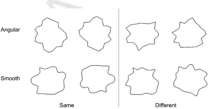
On each trial, there was a pair of shapes presented: one to the left and one to the right of fixation. The distance between the centers was 320 pixels. Examples of stimuli are shown inFigure 5. Stimuli are available for download fromhttps://osf.io/4278q/.
Experimental design and procedure. A 2⫻2⫻2 design was employed. The within-subjects factors were Shape (angular, curved) and Congruency (same, different). The between-subjects Figure 4. Average gradient and edge density as a function of shape and number of vertices. Scatterplots with
regression slopes showing the increase in response time (s) as a function of gradient and edge density. See the online article for the color version of this figure.
Figure 5. Experiment 2a: Examples of angular and smooth stimuli. The first panel shows examples in which the pair of shapes matches (“same”), and the second panel shows examples in which the pair did not match (“different”).
This
document
is
copyrighted
by
the
American
Psychological
Association
or
one
of
its
allied
publishers.
This
article
is
intended
solely
for
the
personal
use
of
the
individual
user
and
is
not
to
be
disseminated
broadly.
7
CURVATURE AND SHAPE PROCESSING
O C
N O
L L
I O
N R
E
F5 AQ: 19
factor was Hand Mapping: Half of the participants used the right hand to respond “same” and the left hand to respond “different,” and the other half of the participants did the reverse. No pair of stimuli was ever presented twice. The experiment lasted approxi-mately 30 min.
The experiment began with the instructions followed by the practice session (six trials). Each trial started with a fixation cross at the center of a white background. This fixation lasted randomly between 600 and 1,600 ms. After that, the pair of shapes appeared and remained on screen until response. In total, there were 180 experimental trials. Other aspects of the procedure were the same as in Experiment 1.
Analysis. A mixed ANOVA was performed with Shape (an-gular, curved) and Congruency (same, different) as within-subjects factors and Key Mapping (mapping of right and left hands to the same/different responses) as a between-subjects factor.
The dependent variable was the response time. Only correct responses were analyzed in the ANOVA. Errors were 4% of the total. In addition, responses above 4,381 ms were removed (two standard deviations above the mean, 1.8% of the trials). After this process, the average response time was 1,388 ms and the standard deviation was 760 ms. In addition to the analysis on response time, we also used a signal detection theory approach and comparedd= andc=measures for sensitivity and bias (Macmillan & Creelman, 2004).
Results and Discussion
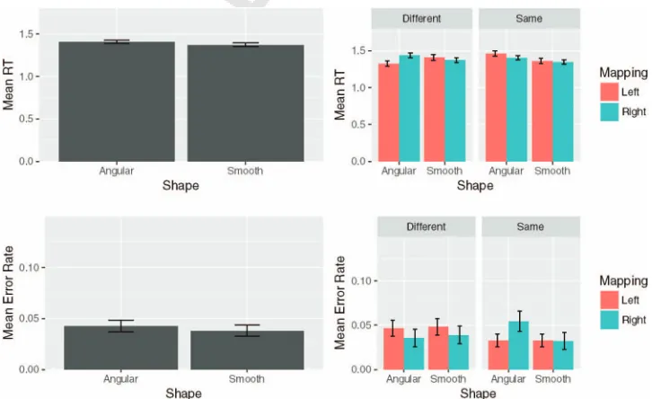
The results are illustrated inFigure 6. The effect of shape in the ANOVA was marginal,F(1, 24) ⫽3.93, p⬍.059, p2⫽ 0.14. There was an interaction between shape and congruency, F(1, 24)⫽5.58,p⬍.027,p2⫽0.19. Finally, there was a three-way
interaction between shape, congruency, and key mapping, F(1, 24)⫽6.12,p⬍.021,p2⫽0.20. The pattern for response time can be compared with the pattern for errors inFigure 6. Error rate was low, and there was no evidence of a speed–accuracy trade-off.
Thed=values were 3.84 for angular shapes and 2.88 for smooth shapes. Thec=was used as a measure of bias and the values were 0.015 for angular shapes and⫺0.004 for smooth shapes. Positive values indicate a bias to respond different and negative values a bias to respond same. Attest analysis did not confirm any signifi-cant difference between the two shapes in terms of sensitivity, t(25)⫽ ⫺0.70,p⫽ .490, or bias,t(25)⫽1.11,p⫽.278. This analysis found mean differences that were consistent with the analysis of response time, but it was not conclusive, as level of performance was high, and therefore d= values suffered from a ceiling effect.
Let us compare the results of Experiment 2a with those of Experiment 1. Responses to shapes with smooth contours were only slightly faster than responses to angular contours (by 26 ms). We have to consider this together with the interaction between shape and congruency. A tendency to respond faster when pro-ducing a “same” rather than a “different” response was associated with the smooth contours. This can be seen as consistent with the results from Experiment 1, because in that study, participants had to produce a positive response (i.e., produce a key press) to either of the two shapes, and they were faster for the smooth contours. It may be easier to produce a positive response to smooth contours, and a negative response to angular contours, in agreement with the results from the measure of approach/avoidance (Palumbo et al., 2015).
The three-way interaction complicates the pattern. Perhaps not surprisingly, there was a tendency to respond more quickly if the
Figure 6. Results of Experiment 2a. On the left, performance is plotted as a function of shape (above: response time; below: errors). On the right, the graph shows the three-way interaction between Shape, Congruency, and Key Mapping. Mapping right means the response “same” was given with the right hand. Mapping left means the response “same” was given with the left hand. Error bars are⫾1 SEM. See the online article for the color version of this figure.
This
document
is
copyrighted
by
the
American
Psychological
Association
or
one
of
its
allied
publishers.
This
article
is
intended
solely
for
the
personal
use
of
the
individual
user
and
is
not
to
be
disseminated
broadly.
F6
“same” response is associated with the right hand (by 211 ms), although key mapping, a between-subjects variable, was not sig-nificant as a main effect. But this role of key mapping manifested itself in terms of making the other differences less pronounced for the group of participants who responded “same” using their right hand.
Experiment 2b: Shape Difference Task
We conducted a second version of the shape matching experi-ment. There were two main modifications. The main change was about orientation: When a pair of identical shapes was presented, one was always rotated 180° compared with the other. We rea-soned that this forced the observer to a more global processing of the shape, perhaps by means of a mental rotation and a comparison of the structural description of the whole object. We also predicted that the task would be harder and the response time would be longer.
The second change was about the match of the stimuli in terms of perimeter length. In Experiments 1 and 2a, we used stimuli with similar area and perimeters, but because of how smooth shapes were generated, they had a slightly longer perimeter compared with angular stimuli. In Experiment 2b, we decided to match perimeter length precisely. Therefore, we prepared stimuli so that each angular shape had a corresponding smooth shape with the same total perimeter. In all other respects, Experiment 2b was the same as Experiment 2a.
Method
Participants. Twenty-six participants took part in Experiment 2b (Mage⫽28 years; one left-handed; 19 females). All partici-pants had normal or corrected-to-normal vision and provided a written consent for taking part. The experiment was approved by the Ethics Committee of the University of Liverpool and was conducted in accordance with the Declaration of Helsinki (2008).
Stimuli and apparatus. The stimuli were generated using a procedure similar to that in Experiment 2a, and the apparatus was the same. On each trial there was a pair of shapes presented, one to the left and one to the right of fixation. For each pair of angular shapes in one trial, the total length of the perimeter was matched to a pair of smooth shapes in another trial. On average, total perimeter was 742 pixels (for angular and for smooth shapes, and also for same and different trials). The distance between the centers was 320 pixels. Examples of stimuli are shown inFigure 7. Stimuli are available for download from:https://osf.io/4278q/.
Experimental design and procedure. A 2⫻2⫻2 design was employed. The within-subjects factors were Shape (angular, curved) and Congruency (same, different). The between-subjects factor was Hand Mapping: Half of the participants used the right hand to respond “same” and the left hand to respond “different,” and the other half of the participants did the reverse. No pair of stimuli was ever presented twice. The experiment lasted approxi-mately 30 min. The procedure was the same as in Experiment 2a. Analysis. A mixed ANOVA was performed with Shape (an-gular, curved) and Congruency (same, different) as within-subjects factors and Key Mapping (mapping of right and left hands to the same/different responses) as a between-subjects factor.
The dependent variable was the response time. Only correct responses were analyzed in the ANOVA. Errors were 10.4% of the total. In addition, responses above 5,382 ms were removed (2SDs above the mean, 4% of the trials). After this process, the average response time was 1,999 ms and the standard deviation was 1,013 ms. In addition to the analysis on response time, we also used a signal detection theory approach and comparedd=andc=measures for sensitivity and bias.
Results and Discussion
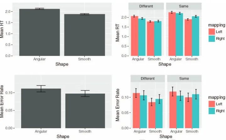
The results are illustrated inFigure 8. There was a significant effect of shape,F(1, 24)⫽48.38,p⬍.001,p2⫽0.67, an effect of congruency, F(1, 24) ⫽ 9.51, p ⫽ .005, p2 ⫽ 0.28, and a
Figure 7. Experiment 2b: Examples of angular and smooth stimuli. The first panel shows examples in which the pair of shapes matches (“same”), and the second panel shows examples in which the pair did not match (“different”). Note the difference in orientation (180°) in the matching pair. Perimeter length was matched so that each smooth subset had a matched angular subset. In these examples, the perimeter is 742 pixels. In the experiment, values ranged between 647 and 814 pixels.
This
document
is
copyrighted
by
the
American
Psychological
Association
or
one
of
its
allied
publishers.
This
article
is
intended
solely
for
the
personal
use
of
the
individual
user
and
is
not
to
be
disseminated
broadly.
9
CURVATURE AND SHAPE PROCESSING
AQ: 20
F7
F8
two-way interaction between shape and key mapping,F(1, 24)⫽ 6.21,p⫽.020,p2⫽0.21. The pattern for response time can be compared with the pattern for errors inFigure 8. Error rate was higher than in Experiment 2a, but there was no evidence of a speed–accuracy trade-off.
Thed=values were 2.67 for angular shapes and 2.85 for smooth shapes. Thec=was used as a measure of bias and the values were 0.001 for angular shapes and 0.020 for smooth shapes. Positive values indicate a bias to respond different and negative values a bias to respond same. At-test analysis did not confirm a significant difference between the two shapes in terms of sensitivity, t(25)⫽ ⫺1.66,p⫽.10,9 or bias,t(25)⫽ ⫺0.70,p⫽.490. As for Experiment 2a, there were some limitations due to ceiling effects but not to the same extent.
The results of Experiment 2b were in the same direction, but more clear-cut, than those from Experiment 2a. The task was much harder, and observers were forced to perform a more global anal-ysis of the shape because the “same” pair was presented with different orientations. Responses to shapes with smooth contours were faster than responses to angular contours (by 235 ms). More-over, the tendency to respond faster when producing a “same” rather than a “different” response in the case of smooth contours was not significant (i.e., no significant interaction between shape and congruency).
Experiment 3: Symmetry
In Experiments 2a and 2b, we used a task in which two shapes had to be compared. This can be thought of as a detection of a translated or rotated shape. In Experiment 3, we used a pair of contours and asked observers to compare them and to detect bilateral symmetry. The task is therefore similar to that of Exper-iment 2, in that the global shape is relevant. Also, again consistent
with Experiment 2, the distinction between smooth and angular was not relevant for the task. Experiment 3 is, however, different in what type of correspondence the observer had to detect. Con-tours could be matched under a reflection, and were therefore symmetrical, or they could be unrelated. In addition, the contours were closed to form a single object in one condition or they were part of two separate objects in another condition. This factor has been found to affect detection of symmetry in previous studies (Baylis & Driver, 1995;Bertamini, Friedenberg, & Kubovy, 1997; Corballis & Roldan, 1974).
Method
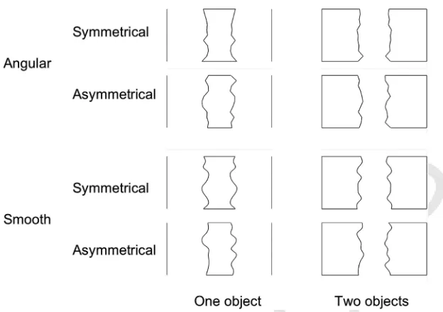
Participants. Twenty-six participants took part in Experiment 3 (Mage⫽29.4 years; one left-handed; 14 females). All partic-ipants had normal or corrected-to-normal vision and provided a written consent for taking part. The experiment was approved by the Ethics Committee of the University of Liverpool and was conducted in accordance with the Declaration of Helsinki (2008). Stimuli and apparatus. The stimuli were generated using a procedure similar to that of Experiment 1. Instead of closed shapes, we generated pairs of vertical contours with 10 vertices. They were shown as black contours on a white background. There was always a context of additional straight lines. One context joined the two contours so as to form a single vertically oriented object; we call this the one-object condition. The other context joined the contours to form two closed shapes with an empty space in between the contours; we call this the two-objects condition. Examples of stimuli are shown inFigure 9. Stimuli are available for download fromhttps://osf.io/4278q/.
Experimental design and procedure. A 2⫻2⫻2 design was employed. The within-subjects factors were Shape (angular, curved), Closure (one object, two objects), and Symmetry (sym-Figure 8. Results of Experiment 2b. On the left, performance is plotted as a function of shape (above: response
time; below: errors). On the right, the graph shows the three-way interaction between shape, congruency, and key mapping. Error bars are⫾1 SEM. See the online article for the color version of this figure.
This
document
is
copyrighted
by
the
American
Psychological
Association
or
one
of
its
allied
publishers.
This
article
is
intended
solely
for
the
personal
use
of
the
individual
user
and
is
not
to
be
disseminated
broadly.
O C
N O
L L
I O
N R
E
metric, asymmetric). The between-subjects factor was the Key Mapping: Half of the participants used the right hand to respond “symmetrical” and the left hand to respond “asymmetrical,” and the other half of the participants did the reverse. The experiment lasted approximately 30 min.
The experiment began with the instructions followed by the practice session (eight trials). Each trial started with a fixation cross. This fixation lasted randomly between 500 and 1,500 ms. After that, the stimulus appeared and remained on screen until response. In total, there were 176 experimental trials. Other aspects of the procedure were the same as in Experiment 1.
Analysis. A mixed ANOVA was performed with Shape (an-gular, curved), Closure (one object, two objects), and Symmetry (symmetric, asymmetric) as within-subjects factors and Key Map-ping (mapMap-ping of right and left hands to the responses) as a between-subjects factor.
The dependent variable was the response time. Only correct responses were analyzed in the ANOVA. Errors were 4.7% of the total. Responses above 2,306 ms were removed (2SDs above the mean, 3.5% of the trials). After this process, the average was 839 ms and the standard deviation was 347 ms. In addition to the analysis on response time, we also used a signal detection theory approach and comparedd=andc=measures for sensitivity and bias.
Results and Discussion
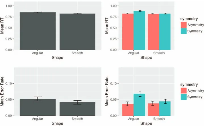
The mean response times are illustrated in Figure 10. The ANOVA confirmed a significant main effect of shape,F(1, 24)⫽ 12.74, p ⫽ .002, p2 ⫽ 0.35 (responses were faster to smooth contours) and a significant effect of closure,F(1, 24)⫽12.58,p⫽ .002,p2⫽0.34 (responses were faster for one object). There was an interaction between shape and symmetry,F(1, 24)⫽6.05,p⫽ .02,p2⫽0.20, and an interaction between shape, symmetry, and key mapping,F(1, 24)⫽8.22,p⫽.008,p2⫽0.25. We did not
find the expected interaction between symmetry and closure,F(1, 24)⫽1.60,p⫽.218, although in terms of mean response time, the difference is in the predicted direction (a relative advantage for symmetry within a single object).
The pattern of results is shown inFigure 10. In relative terms, people are fast when they make positive responses (“same” or “symmetry”) to the smooth shapes and negative responses (“dif-ferent” or “asymmetrical”) to the angular shapes. The pattern for response time can be compared with the pattern for errors. The error rate was low, and there was no evidence of a speed–accuracy trade-off.
Thed=values were 3.39 for angular shapes and 3.50 for smooth shapes. Thec=was used as a measure of bias and the values were 0.034 for angular shapes and 0.002 for smooth shapes. Negative values indicate a bias to respond “symmetry” and positive values a bias to respond “asymmetry.” At-test analysis did not confirm a significant difference between the two types in terms of sensitivity, t(25)⫽ ⫺1.91,p⫽.067. There was, however, a difference for the bias,t(25)⫽2.12,p⫽.044. As for Experiment 2, this analysis suffered the limitation of high performance and a ceiling effect, but it does support the conclusion that for smooth shapes, there was more of a bias to produce a positive response (in this case for “symmetry”) than for angular shapes.
General Discussion
We have compared abstract shapes with sharp angles (irregular polygons) and similar shapes with smooth contours. In the first study, we tested a speeded response to the onset of the stimulus from a specific category (angular or smooth). Observers could produce the response quickly (overall average response time was 692 ms). Responses to shapes with smooth contours were faster compared with angular shapes (by 50 ms).
Figure 9. Experiment 3: Examples of the stimuli: On the top, angular stimuli, and on the bottom, smooth stimuli. The set of four stimuli on the left show the one-object condition, and the four stimuli on the right show the two-objects condition.
This
document
is
copyrighted
by
the
American
Psychological
Association
or
one
of
its
allied
publishers.
This
article
is
intended
solely
for
the
personal
use
of
the
individual
user
and
is
not
to
be
disseminated
broadly.
11
CURVATURE AND SHAPE PROCESSING
F10
In the second study, two shapes had to be compared to decide whether they were identical or different. The shapes were outlines and each pair had either both angular or both smooth contours. The task was harder and required an analysis of the whole shape, in particular in Experiment 2b, in which shapes were both translated and rotated (average response time was 1,388 ms in Experiment 2a and 1,999 ms in Experiment 2b). The task in Experiment 2a was easy and probably led to ceiling effects. Moreover, as the match was direct (side by side), it did not force a global processing of the shapes as much as Experiment 2b. In Experiment 2a, there was only a trend for participants to be faster when responding to shapes with smooth contours. There was also an interaction between the match between the shapes and the type of shape. Specifically, participants were relatively faster to respond “same” for smooth contours and to respond “different” for angular contours. The advantage for smooth shapes, on the other hand, was clear in Experiment 2b: Responses to smooth shapes were faster by 235 ms.
In the final experiment (Experiment 3), observers had to report whether a pair of contours were bilaterally symmetrical or not. This task was slower than the task of Experiment 1 but faster than the task of Experiments 2a and 2b (average response time was 933 ms). Again, responses were faster for smooth contours than for angular contours (by 30 ms). There was also a bias to respond “symmetry,” which was stronger for smooth shapes compared with angular shapes. Note that in Experiments 2a, 2b, and 3, the difference in shape (angular or smooth) was completely task irrelevant. Observers were making a judgment about an orthogonal dimension.
How can we explain faster responses to smooth contours con-sistently across three different tasks? Given the way the stimuli were generated, the two conditions (angular or smooth) were comparable in terms of overall size (with a slightly larger area for
smooth shapes) and in terms of number of convexities and con-cavities. Differences in perimeter length were small, and in Ex-periment 2b, the stimuli were prepared so as to match perimeter length exactly (using pairs of smooth and angular stimuli matched on this variable). When we varied the number of vertices in Experiment 1, shapes with more vertices (which also appear more angular) were responded to more slowly. It is important to note that the smooth shapes are objectively more complex, in particular in terms of edge orientation along the contour. In a delayed matching task with abstract shapes, Kayaert and Wagemans (2009) found that responses were slower and less accurate when com-plexity increased. However, smooth contours are not judged to be more complex. On the contrary, they are subjectively judged as less complex (Bertamini et al., 2016, Experiment 1). This may be because a smooth contour is seen as a single line; by contrast, a polygon is segmented in a number of individual lines and there-fore, perhaps, individual parts.
We have argued that angular shapes, and polygons in particular, are simpler than our smoothed polygons. There are many ways to operationalize complexity, and there is a large literature on com-plexity including the analysis of statistical image properties. The concept of complexity is related to other aspects like fractal dimension and symmetry (Graham & Redies, 2010). The objective complexity of the smooth stimuli was documented for the stimuli in Experiment 1 in an additional post hoc analysis. This was based on the computation of two objective measures of complexity, referred to ascomplexityandedge density. The type of shape was the best predictor of response time also in the context of complex-ity as a second predictor.
The results show faster responses to smooth shapes. This finding is interesting, not related to objective complexity, and likely re-lated to the subjective simplicity of these shapes and to the fact that people have a preference for smooth shapes. Previous findings in Figure 10. Results of Experiment 3. On the left, performance is plotted as a function of shape (above: response
time; below: errors). On the right, the graph shows the two-way interaction between shape and symmetry. Error bars are⫾1 SEM. See the online article for the color version of this figure.
This
document
is
copyrighted
by
the
American
Psychological
Association
or
one
of
its
allied
publishers.
This
article
is
intended
solely
for
the
personal
use
of
the
individual
user
and
is
not
to
be
disseminated
broadly.
O C
N O
L L
I O
N R
E
AQ: 22
the literature were mixed, and they come from studies that did not set out to directly test the question of speed of processing as a function of contour type. InBar and Neta (2006), participants were asked to give a fast preference response (like/dislike) after a brief presentation of images (84 ms). There was a difference in prefer-ence but no significant differprefer-ence in response times. For real objects and for meaningless patterns, the difference between smooth and angular conditions was very small (5 ms and 1 ms, respectively). In Experiment 4 inBertamini et al. (2016), there was an overall effect of shape on response time, but this was modulated by type of response. There was no difference between angular and smooth shapes for approach responses, and slower responses to smooth shapes for avoidance responses. In other words, there was difficulty in producing a negative (avoidance) response to smooth stimuli. Nevertheless, this difference raises questions about how to compare different tasks, and in some conditions, responses may be slower to smooth stimuli. Note that the approach/avoidance task required an explicit evaluation of contour type: Observers had to first decide whether the shape was smooth or angular, and then produce different responses. Therefore, this evidence supports our choice of using tasks in which shape was not task relevant. Next, we provide some context and speculation about the origin of this advantage.
In the introduction, we mentioned that the principles of grouping introduced by Gestalt psychologists (for a review, seeWagemans et al., 2012) include proximity and good continuation. Contour integration can be studied by manipulating local orientation of a set of elements. When these elements are aligned along a smooth path (collinearity), sensitivity in a contour detection task increases (Field et al., 1993). The stimuli typically used in these studies have become known as snakes (similar local orientation) and ladders (orthogonal local orientation;Bex et al., 2001). Our stimuli are fundamentally different, but it is relevant to note that snakes are related to smooth contours, in that along the contour, changes in orientation are always small. If it is easier to integrate contours of this type, this advantage may also lead to faster responses and to a perception of these shapes as less complex. However, angular shapes have good continuity for most of their length. The discon-tinuity is localized at the vertices. If these local discontinuities are the key difference, then any prediction based on contour integra-tion should be mainly a funcintegra-tion of number of vertices. Our experiments did not test this factor directly. When number of vertices was manipulated (Experiment 1), there was no overall interaction between type of shape and number of vertices. More-over, for preference tasks, number of vertices does not seem to be important. For example, smooth curves (parabola) are preferred to straight lines with or without vertices (Bertamini et al., 2016, Experiment 3). A similar argument can be made about the hypoth-esis that segmentation of the shape into separate lines is an im-portant factor. If it is true that polygons are perceived as composite objects, this could explain the fact that they are judged as more complex and, perhaps, that responses are slower. This hypothesis predicts a difference in behavior as a factor of number of vertices on all tasks.
With respect to the importance of curvature in perception, it is worth noting that curvature plays an important role in how shape is encoded in the brain (Pasupathy & Connor, 2002), and contour information—in particular, convexities and concavities—affects perceived part structure (Bertamini & Wagemans, 2013;Hoffman
& Richards, 1984). In terms of experimental evidence, differences in contour curvature affect visual search efficiency (Hulleman, te Winkel, & Boselie, 2000;Kristjánsson & Tse, 2001), shape match-ing (Bertamini, 2008;Garrigan & Kellman, 2011), shape afteref-fects (Gheorghiu & Kingdom, 2008;Hancock & Peirce, 2008), target detection (Barenholtz & Feldman, 2003), and perceived part structure (Barenholtz, Cohen, Feldman, & Singh, 2003;Bertamini & Croucher, 2003). There are also well-known illusions in which straight lines are perceived as curved (Hering, 1861;Oppel, 1855) or curved lines are perceived as straight (Bertamini & Kitaoka, 2018;Takahashi, 2017).
A more fundamental point has to do with the visual environ-ment. Polygons are simple in terms of geometry and in terms of how they can be drawn on paper or by computers; however, they are very artificial and unnatural. If contours are projected outlines of surface occlusion, and, in particular, surface self-occlusion, then smooth contours are more common and natural (for smooth sur-faces;Hoffman & Richards, 1984;Koenderink, 1984, 1990). By analyzing images of the natural environment in terms of local edge orientationsSigman, Cecchi, Gilbert, and Magnasco (2001)found long-range correlations. There was a pattern of cocircularity for orientation, and this pattern extended over the entire visual field. A follow-up analysis by Chow, Jin, and Treves (2002)came to a slightly different conclusion: The data may simply “indicate that there are many closed smooth contours in natural visual scenes” (p.●●●). The important point is that, as Sigman et al. suggested, properties of the visual system that integrate edge information match regularities in the environment.
The relative advantage of the visual system to process smooth contours may therefore be se