Stability Analysis of Artificial Bee Colony Optimization Algorithm

Stability Analysis of Artificial Bee Colony Optimization

Algorithm

Jagdish Chand Bansal

, Anshul Gopal

South Asian University, New Delhi, India

Atulya K. Nagar

Liverpool Hope University, UK

January 9, 2018

Abstract

Theoretical analysis of swarm intelligence and evolutionary algorithms is relatively less explored area of research. Stability and convergence analysis of swarm intelligence and evo-lutionary algorithms can help the researchers to fine tune the parameter values. This paper presents the stability analysis of a famous Artificial Bee Colony (ABC) optimization algorithm using von Neumann stability criterion for two-level finite difference scheme. Parameter selec-tion for the ABC algorithm is recommended based on the obtained stability condiselec-tions. The findings are also validated through numerical experiments on test problems.

Keywords

Artificial Bee Colony (ABC) Algorithm, Stability Analysis, Finite Difference Scheme, Parameter Selection, Stable Range

1

Introduction

Over past few years, algorithms taking inspiration from natural phenomena have attracted re-searchers. Particle Swarm Optimisation (PSO) algorithm [26], Artificial Bee Colony (ABC) op-timization algorithm [21], Differential Evolution (DE) algorithm [37], Harmony Search Algorithm (HSA) [17], Gravitational Search Algorithm (GSA) [33] are few popular algorithms of this class. Study has shown that these algorithms are considered as efficient solver of complex optimization problems. Artificial Bee Colony (ABC) optimization algorithm is a prominent candidate in this field of nature inspired algorithm. It takes inspiration from the intelligent foraging behaviour and information sharing capability of honey bees [24][7]. Firstly it was introduced by Karaboga in 2005 for continuous optimization problems and later it was also modified to solve discrete optimization problems [25][27].

Recently various other variants of the ABC algorithm have been proposed which includes Chaotic ABC [4], ABC algorithm for multiobjective optimization problems [3], for constrained optimization problem [22] and various hybrid ABC algorithms [15][32][6]. The ABC algorithm is applied for solving various continuous and discrete optimization problems in the areas related to neural networks [23][28], structural engineering[13], assignment problem [31][8], image processing [14], network topology design [35] and forecasting stock markets [19].

Various researchers have worked on these meta-heuristic search algorithms analytically and experimentally. However, one of the important aspect related to such algorithms is to ensure that the error generated by them are bounded. Hence, stability analysis plays a significant role in the theoretical study of these algorithms. However, a little work has been done in the area of stability analysis of this class of algorithms. Attempts have been made to analyse the stability behaviour of few algorithms which includes Particle Swarm Optimisation (PSO) algorithm using

Z-transformation [20] [30][36], Differential Evolution (DE) algorithm by using Lyapunov’s stabil-ity theorem and von Neumann stabilstabil-ity criterion [12][18], Bacterial Foraging Optimization (BFO) algorithm using Lyapunov’s stability condition and eigen value method [11][9], Ant Colony Opti-mization (ACO) algorithm [1] and Gravitational Search algorithm (GSA) using passivity theorem and Lyapunov’s stability condition [16].

In recent past, studies have been done for parameter selections of the ABC algorithm in order to get better optimization results [2][29]. Also effect of parameters like dimension, colony size, region scaling and effect of limit or abondment counter (AC) on the ABC algorithm has already been discussed in [2]. To the best of authors’ knowledge, no attempt has yet been made for the stability analysis of the Artificial Bee Colony (ABC) optimization algorithm. This paper is an attempt to discuss the stability of the ABC algorithm for solving continuous optimization problems, using von Neumann stability criterion for two level finite difference scheme and to propose parameter selection based on the stability analysis. Stability of discrete version of ABC algorithm can be done in similar way because it uses the same position update equation in order to get new candidate solutions.

Rest of the paper is organised as follows: Original ABC algorithm is explained in section 2. Section 3 presents the motivation for mathematical analysis of the ABC algorithm and provide details of von Neumann stability criteria for two level finite difference scheme. In section 4 stability analysis of the ABC algorithm is carried out. Numerical experiments and results are discussed in section 5 and the study is concluded in section 6.

2

Artificial Bee Colony (ABC) Optimization Algorithm

Artificial Bee Colony (ABC) optimization algorithm is a population based optimization algorithm and uses an iterative method to achieve global maximum or minimum. The bee hive constitutes mainly three kinds of bees; employed bees, onlooker bees and scout bees. Exploitation of nectar source is done by employed bees and onlooker bees whereas scout bees explore the search region. In Artificial Bee Colony (ABC) optimization algorithm, the number of nectar sources equals the number of employed bees. Also, the number of employed bees and onlooker bees are equal. The ABC algorithm has four phases; initialization, employed bee, onlooker bee and scout bee.

2.1

Intialization

Artificial Bee Colony (ABC) optimization algorithm starts with random selection of the food source which corresponds to the potential solution. The initial solutions are produced for employed bees by using the equation:

xi,j=xminj +µ(x max j −x

min

j ), i= 1,2,3...N, j= 1,2,3...D (1)

where, xi,j is the jth dimension of theith employed bee/food source; xmaxj andxminj are the

upper and lower bounds of thejth_{parameter, respectively;µis a random number in the range of}

[0,1]. Nis the number of food source, i.e. swarm size andDis the dimensionality of the considered optimization problem. Also, the abandonment counter (AC) of each employed bee is reset in this phase.

2.2

Employed Bee Phase

In this phase, for each employed bee a new candidate solution is produced. First, the solution of the employed bee is copied to new candidate solution (vi =xi). Then, one parameter of the

solution is updated by using the equation:

vi,j=ψxi,j+φ(xi,j−xr,j), i, r∈

1,2,3..., N , j∈

1,2,3..., D and i6=r (2)

Here jth _{parameter is selected randomly for updation and the coefficient ψ is taken as unity in}

original ABC algorithm. This is done by randomly selecting a candidatexr in the neighbourhood

of ith _{candidate. φ is the random number ranging in the interval [−1,1], N is the number of}

f iti =

1

1+fi, iffi≥0

1 +abs(fi), otherwise

where f iti is the fitness value ofith candidate solution, fi is the objective function value of

ith employed bee. If the fitness value of the updated candidate solution is better than the fitness value of current solution then the current solution is replaced with candidate solution and the abandonment counter of the employed bee is reset to zero, otherwise abandonment counter is increased by one.

2.3

Onlooker Bee Phase

In ABC algorithm, to improve the solution each onlooker bee selects an employed bee. The

probability of selectingith _{employed bee is calculated using Roulette wheel selection:}

pi=

f iti

PN

j=1f itj

(3)

wherepiis the probability of selectingithemployed bee. The solution of selected employed bee

is improved by the onlooker bees by using equation (2). If the fitness value of new solution found by the onlooker bee is better than the employed bee, the onlooker bee is changed with the employed bee and the abandonment counter of the employed bee is reset to zero otherwise, abandonment counter is increased by one.

2.4

Scout Bee Phase

The abandonment counters of all employed bees are checked with a predefined limit. The employed bee, which fails to improve the solution before reaching the limit, becomes scout bee. Hereafter, equation (1) is used to the produce solution for scout bee and the abandonment counter is reset. The scout bee then becomes employed bee. Therefore, scout bee prevents the stagnation of employed bee population.

3

Motivation and Stability Criteria

3.1

Motivation

Nature inspired optimization algorithms are used to solve real world optimization problems. The algorithms provide near optimal solution and therefore the error in the obtained solution should be bounded. It is not necessary that the error generated by an iteration is always less than that of the previous iteration. It may increase indefinitely. In this case, we say that the iterative procedure is unstable. Therefore, it is worth to investigate the stability of the algorithm to bound the generated error. In the considered ABC algorithm, greedy selection is applied in both employed bee phase and onlooker bee phase which plays a vital role in reducing the error. In addition to that candidate solution is selected using fitness based probability, which also reduces the error. But upto authors’ knowledge, no attempt has yet been made to restrict the error by deriving conditions on the parametersφandψgiven in equation (2). The position update equation of ABC algorithm consists of two user defined parametersφandψ. Therefore apart from greedy selection and fitness based probability selection, the value ofφandψcan also play a significant role in the ABC search process. Hence the study of finding most suitable stable range for φandψ is important. Further with experimental results on benchmark test problems, we can analyse that though selection of candidate solution based on fitness based probability criteria and greedy selection helps in reducing error but with proper selection of parameters φandψthe error can be reduced in less number of iterations as compared to the case when there is no restriction on these parameters. The study can serve as a recommendation to set the range of parametersφandψfor any proposal on modification of ABC algorithm.

Section 4 presents the stability analysis of ABC algorithm by analysing the position update equation (2) of ABC algorithm. The von Neumann stability criteria for two level finite difference scheme is applied to perform the stability analysis of equation (2) and hence of ABC algorithm.

3.2

von Neumann Stability Criterion

The linear partial differential equation considered in this paper for an initial value problem will be represented by:

∂u

∂t +Lx(u) = 0

whereLx(u) represents a linear spatial differential operator anduis the dependent variable, which

is a function of independent variablesxandt.

A two-level difference scheme for this linear partial differential equation can be written in the form [39]:

mr X

q=−ml

Bqunj++1q = nr X

q=−nl

Aqunj+q (4)

whereml, mr, nlandnrare non-negative integers. jandnrepresents number of grid points in the

direction of xandtrespectively.

The von Neumann stability procedure consists of replacing each termun_j of the difference equation by kth Fourier component of a harmonic decomposition of un_j, i.e. by vn(k)eιkj∆x, wherevn(k) denotes thekth_{Fourier coefficient andι=}√_−1.

The (n)th _{and (n+ 1)}th_{Fourier coefficients of harmonic decomposition ofu}n

j are related by

vn+1_{(k) =g(k)v}n_(k)

whereg(k) is the amplification factor of the finite difference scheme.

For a two level finite difference scheme with only one dependent variable, the necessary and sufficient condition for stability is |g(k)| ≤1 for all values of k. If |g(k)| = 1 for all k, then the difference scheme is said to be nondissipative or marginally stable, and if|g(k)|>1 for somek, the scheme is unstable [34]. The stability criterion for finite difference scheme (4) can also be presented as below.

For two-level schemes, the square of the magnitude of amplification factor, i.e. |g(k)|2 _can

always be expressed as a rational function given below [39]:

|g(k)|2_{= 1−4z}rS(z)

P(z) (5)

where,

z=sin2(θ/2), θ=k∆x (6)

S(z) =

s

X

i=0

αizi, α0=S(0)6= 0 (7)

P(z) =

d

X

i=0

βizi >0, β0=P(0) = 1 (8)

Here, α0, α1, ..., αsand β0, β1, ..., βd are constants. r is a positive integer ands is a non-negative

integer, and they are related by the formula r+s =m. Where, m=max(ml+mr, nl+nr) is

determined by the number of spatial grid points to the left and right ofxjin the difference scheme.

The integerdis non-negative andd=mr+ml.

The polynomialS(z) determines the stability of the given difference scheme. The necessary and sufficient condition for stability is [39]:

S(0)>0, S(z)≥0 f or 0< z=sin2(θ/2)≤1 (9)

In short, the necessary and sufficient condition for the stability of a difference scheme given in (4), with magnitude of amplification factor represented by (5)−(8) can be stated as below: Two level difference scheme (4) is stable iff:

S(0)>0, S(z)≥0 f or 0< z=sin2(θ/2)≤1 (10)

be given by (10).

In the next section, stability analysis has been carried out for Artificial Bee Colony (ABC) optimization algorithm based on the von Neumann stability criterion discussed above.

4

Stability Analysis of ABC Algorithm

The parameter φ plays an important role in the search process of Artificial Bee Colony (ABC) optimization algorithm:

This parameter provides stochastic search in ABC and thus prevents the particles from getting stagnated at local optima.

In Artificial Bee Colony (ABC) optimization algorithm, the solutions are updated using the position update equation (2):

vi,j=ψxi,j+φ(xi,j−xr,j), i, r∈

1,2,3..., N ; j∈

1,2,3..., D and i6=r (11)

If the current iteration counter ist, thenxi,j is thejthdimension of theith candidate solution

at iterationt, whilevi,jis thejthdimension of theithcandidate solution at iteration (t+ 1). In the

original version of ABC algorithm, the coefficientψis taken to be unity. Without loss of generality the above equation can be written as:

xi,j(t+ 1) =ψxi,j(t) + φ(xi,j(t)−xr,j(t)) (12)

In ABC algorithm, the position update equation (12) is implemented component wise, i.e. each dimension of the solution is updated independently. The only link between the dimensions of the problem space is introduced via objective function. Thus, without loss of generality, the algorithm description can be reduced for analysis purposes to the one dimension case as considered in [38][16][11]. Thus equation (12) can be written as:

xi(t+ 1) = (ψ+φ)xi(t)−φxr(t) (13)

where, ris randomly selected solution index different fromi. Sincerandiare non-negative inte-gers in [1, N], thus we can writer=i±awhere,ais random positive integer in the range [1, N].

Hence, equation (13) in the form of difference equation can be written as:

xt_i+1= (ψ+φ)xt_i−φxt_i±a (14)

If the true solution to a problem in ani-tcomputational domain is represented byx=x(i, t), the approximate solution on the nodes of a computational grid will be represented byxl,n=x(il, tn).

In terms of grid pointsxl,nthe difference equation can further be written as:

xn_l+1= (ψ+φ)xn_l −φxn_l±a (15)

In accordance with von Neumann stability procedure, each termxn

l of the difference equation

is replaced by vn_(k)eι(kl∆i)_{, which is thek}th _{Fourier component of a harmonic decomposition of}

xn

l. Here,vn(k) is thekthFourier coefficient in this decomposition. The (n)thand (n+ 1)thFourier

coefficients of harmonic decomposition ofxn

l are related by:

vn+1(k) =g(k)vn(k) (16)

whereg(k) is the amplification factor of the finite difference scheme (15).

The amplification factor of the difference scheme (15) can easily be calculated and is given by [See Appendix A]:

g(k) = (ψ+φ)−φeι((±a)k∆i) (17)

or

g(k) = (ψ+φ)−φeι(θ), where θ= (±ak∆i) (18)

|g(k)|=

q

ψ2_{+ 4φ(ψ+φ)sin}2_{(θ/2) (19)}

Further using necessary and sufficient condition for stability we get

q

ψ2_{+ 4φ(ψ+φ)sin}2_{(θ/2)≤1 (20)}

or

ψ2+ 4φ(ψ+φ)sin2(θ/2)≤1 (21)

or

ψ2≤1−4φ(ψ+φ)sin2(θ/2) (22)

or

ψ2≤1−4φ(ψ+φ) Since, sin2(θ/2)≤1 (23)

Since,xr,j(t) represents the randomly selected candidate solution in the current iteration and

outcome of its difference withxi,j(t) in equation (12) can be either positive or negative. Hence,

without loss of generality equation (12) can be rewritten as:

xi,j(t+ 1) =ψxi,j(t) + φ(xr,j(t)−xi,j(t)) (24)

which can again be written as

xi,j(t+ 1) =ψxi,j(t) − φ(xi,j(t)−xr,j(t)) (25)

As done earlier the amplification factor is given by

g(k) = (ψ−φ) +φeι((±a)k∆i) (26)

or

g(k) = (ψ−φ) +φeι(θ), where θ= (±ak∆i) (27)

By doing the similar mathematical analysis and calculations as done earlier, the necessary and sufficient condition for the stability is given by :

ψ2≤1 + 4φ(ψ−φ) Since, sin2(θ/2)≤1 (28)

Equation (23) and (28) provide the necessary and sufficient conditions for the stability of ABC position update equation (2).

In the next subsection, a special case, i.e. (ψ = 1) is considered which corresponds to the original ABC algorithm. The stable range ofφis recommended for this case as well.

4.1

Stability analysis of ABC algorithm with coefficient

ψ

= 1

We will find the stable range ofφby two different methods. Firstly, by takingψ= 1 in equation (23) and (28) to get the desired range ofφ. Secondly, by using the stability condition from equation (10).

By takingψ= 1 in equation (23) we get −φ(1 +φ)≥0, i.e. φ∈[−1,0]

Similarly, By takingψ= 1 in equation (28) we get

φ(1−φ)≥0, i.e. φ∈[0,1]

By combining the above two results we can conclude that ABC algorithm is stable for φ ∈ [−1,1].

Now, we will use the stability condition as explained in equation (10) to verify the results obtained from first method.

In Artificial Bee Colony (ABC) optimization algorithm, the solutions are updated using the position update equation (2) (ψ is taken as unity):

vi,j =xi,j+φ(xi,j−xr,j), i, r∈

1,2,3..., N ; j∈

If the current iteration counter ist, thenxi,j is thejthdimension of theith candidate solution

at iteration t, while vi,j is the jth dimension of the ith candidate solution at iteration (t+ 1).

Without loss of generality the above equation can be written as

xi,j(t+ 1) =xi,j(t) + φ(xi,j(t)−xr,j(t)) (30)

In ABC algorithm, the position update equation (12) is implemented component wise, i.e. each dimension of the solution is updated independently. The only link between the dimensions of the problem space is introduced via objective function. Thus, without loss of generality, the algorithm description can be reduced for analysis purposes to the one dimension case as considered in [38][16][11]. Thus equation (30) can be written as:

xi(t+ 1) = (1 +φ)xi(t)−φxr(t) (31)

where, ris randomly selected solution index different fromi. Sincerandiare non-negative inte-gers in [1, N], thus we can writer=i±awhere,ais random positive integer in the range [1, N].

Hence, equation (31) in the form of difference equation can be written as:

xt_i+1= (1 +φ)xt_i−φxt_i±a (32)

If the true solution to a problem in ani-tcomputational domain is represented byx=x(i, t), the approximate solution on the nodes of a computational grid will be represented byxl,n=x(il, tn).

In terms of grid pointsxl,nthe difference equation can further be written as:

xn_l+1= (1 +φ)xnl −φxnl±a (33)

In accordance with von Neumann stability procedure, each termxn_l of the difference equation is replaced by vn_(k)eι(kl∆i)_{, which is thek}th _{Fourier component of a harmonic decomposition of}

xn

l. Here,v

n_{(k) is thek}th_{Fourier coefficient in this decomposition. The (n)}th_{and (n+ 1)}th_Fourier

coefficients of harmonic decomposition ofxn

l are related by:

vn+1(k) =g(k)vn(k) (34)

whereg(k) is the amplification factor of the finite difference scheme (33).

The amplification factor of the difference scheme (33) can easily be calculated and is given by [See Appendix A]:

g(k) = (ψ+φ)−φeι(θ), where θ= (±ak∆i) (35)

Further, we can obtain

|g(k)|2= (1 +φ)2+ (φ)2−2φ(w−φ)cosθ (36)

|g(k)|2−1 = 4φ(1 +φ)sin2(θ/2) (37)

where, θ= (±ak∆i)

For two-level schemes, the modulus of square of amplification factor can be expressed in the form of rational function as:

|g(k)|2_{= 1−4z}rS(z)

P(z) (38)

where,

z=sin2(θ/2) , θ= (k∆x) S(z) =Ps

i=0αizi ,α0=S(0)6= 0

P(z) =Pd

i=0βizi , β0=P(0) = 1

Here, ris a positive integer,sanddare non negative integers.

The necessary and sufficient condition for stability as given in equation (10) is [39]:

1. S(0)>0

By comparing equation (37) with equation (38) we get:

S(z) =−φ(1 +φ)

Hence, the necessary and sufficient condition for stability is given by:

−φ(1 +φ)≥0, i.e. φ∈[−1,0]

Since,xr,j(t) represents the randomly selected candidate solution in the current iteration and

outcome of its difference withxi,j(t) in equation (12) can be either positive or negative. Hence,

without loss of generality equation (12) can be rewritten as:

xi,j(t+ 1) =xi,j(t) + φ(xr,j(t)−xi,j(t)) (39)

which can again be written as:

xi,j(t+ 1) =xi,j(t) − φ(xi,j(t)−xr,j(t)) (40)

By doing the similar mathematical analysis and calculations as done earlier, the necessary and sufficient condition for the stability of ABC algorithm is given by :

S(z) =φ(1−φ)≥0 i.e. φ∈[0,1]

So, by combining the above two results, we can easily interpret that necessary and sufficient condition for the stability of update equation of ABC algorithm is that the parameterφmust lie in the interval [−1,1]. In short, the stability of ABC algorithm depends upon the range of parameter φ.

The findings of the stability analysis of Artificial Bee Colony (ABC) optimization algorithm verifies the recommended setting of parameterφin Artificial Bee Colony (ABC) algorithm search process. That is, for the stability of ABC algorithm,φmust be in the range [−1,1].

This stability analysis can further be applied to improve the performance of various advanced variants of ABC, e.g. [5][10]. In [5], Akay et al. introduced an adaptive scaling factor ‘φ’ based on Rechenbergs 1/5th mutation rule. The analysis undertaken in this paper can be used to set the value of coefficient ‘ψ’(refer equation 2) as a function of adaptive scaling factor (ASF). This strategy can further improve the ABC algorithm in terms of accuracy.

Similarly, the stability analysis carried out in this paper can also be applied to set the scaling factors ‘φG’ and ‘φC’ introduced by Das et al. [10] in two different ways:

1. Stability analysis of ABC with two scaling factors ‘φG’ and ‘φC’ can provide a relation

between ‘φG’ and ‘φC’.

2. A relation like equation (23) and (28) among ’ψ’, ’φG’ and ’φC’ can be obtained.

An intensive future research is required for these analyses. Other variants of ABC can also be checked for this kind of relations between proposed coefficientψ and scaling factorφ.

Next section verifies numerically that other ranges of φ are not as efficient as stable range [−1,1].

5

Numerical Experiments

In order to validate our theoretical findings numerically, four different ranges of parameter φare considered. Numerical experiments are performed with φ ∈ [−1,1], φ ∈ [−3,−1], φ∈ [1,3] and φ∈[−2,−1]∪[1,2]. The length of all the ranges are same as the length of stable range. The range [−3,−1] represents the case ifφis selected from left of stable range, while the range [1,3] chooses φfrom the right of stable range. The range [−2,−1]∪[1,2] represents choice of selection ofφfrom left or right of the stable range.

Following three types of numerical experiments are performed:

1. In subsection 5.1, error convergence graphs are plotted .

2. Subsection 5.2, presents evolving performance of the ABC algorithm for four different ranges of parameterφand results are validated through Mann-Whiteny U rank sum test.

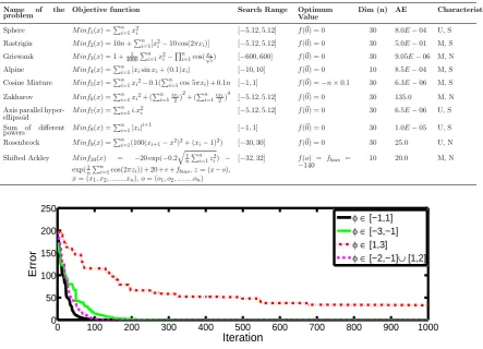
Table 1

List of Test Problems (AE: Acceptable Error,U: Uni-modal,M: Multi-modal,S: Separable,N: Non-separable )

Name of the

problem Objective function Search Range OptimumValue

Dim (n) AE Characteristic

Sphere M inf1(x) =Pin=1x2i [−5.12,5.12] f(~0) = 0 30 8.0E−04 U, S

Rastrigin M inf2(x) = 10n+Pin=1[x2i−10 cos(2πxi)] [−5.12,5.12] f(~0) = 0 30 5.0E−01 M, S

Griewank M inf3(x) = 1 +40001

Pn

i=1x2i−

Qn

i=1cos(√xii) [−600,600] f(~0) = 0 30 9.05E−06 M, N

Alpine M inf4(x) =Pni=1|xisinxi+ (0.1)xi| [−10,10] f(~0) = 0 10 8.5E−04 M, S

Cosine Mixture M inf5(x) =Pni=1xi2−0.1(Pni=1cos 5πxi) + 0.1n [−1,1] f(~0) =−n×0.1 30 6.3E−06 M, S

Zakharov M inf6(x) =

Pn

i=1xi2+ (

Pn

i=1ix2i) 2

+ (Pn i=1ix21)

4

[−5.12,5.12] f(~0) = 0 30 135.0 M, N Axis parallel

hyper-ellipsoid

M inf7(x) =Pni=1i.x2i [−5.12,5.12] f(~0) = 0 30 6.5E−06 U, S

Sum of different

powers M inf8(x) =

Pn

i=1|xi|i+1 [−1,1] f(~0) = 0 30 1.0E−05 U, S

Rosenbrock M inf9(x) =Pni=1(100(xi+1−x2)2+ (xi−1)2) [−30,30] f(~0) = 0 30 25.0 U, N

Shifted Ackley M inf10(x) = −20 exp(−0.2

q

1

n

Pn

i=1zi2) −

exp(1

n

Pn

i=1cos(2πzi)) + 20 +e+fbias,z= (x−o), x= (x1, x2, ...xn),o= (o1, o2, ...on)

[−32,32] f(o) = fbias = −140

10 20.0 M, N

0 100 200 300 400 500 600 700 800 900 1000

0 50 100 150 200 250

Iteration

φ∈ [−1,1] φ∈ [−3,−1] φ∈ [1,3]

φ∈ [−2,−1]∪ [1,2]

Fig. 1. Convergence graphs forf1 with various ranges ofφ.

5.1

Convergence

In order to see convergence behaviour of the ABC algorithm with different ranges of parameterφ, experiments are performed over 10 test problems given in Table 1. The test problems of Table 1 consists of separable, non separable, uni-modal and multi-modal optimization functions.

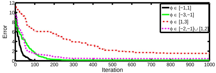
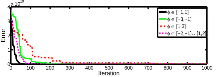
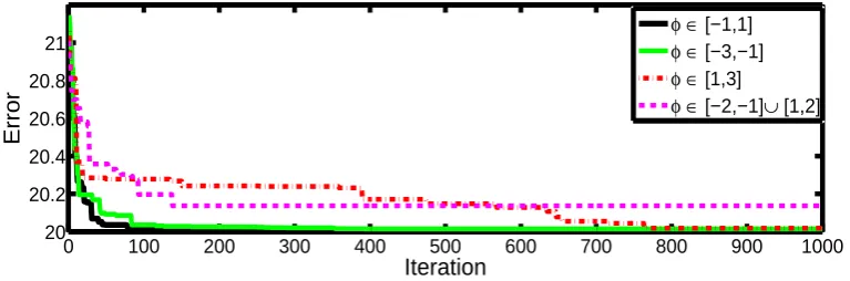
Figure 1 to 10 show convergence graphs of the ABC algorithm over 1000 iterations. It can be concluded that in ABC algorithm greedy selection and fitness based probability selection is done to get improved results in each iteration hence, error is decreasing with increase in iteration for almost every range of parameter φ. Graphs clearly show that for theoretically proposed stable range of parameter φ, i.e. [-1,1], the algorithm takes less number of iterations to reach to near optimal solution as compared to other ranges ofφ. Hence the proposed stability criteria for ABC algorithm plays a vital role in convergence behaviour of ABC algorithm.

5.2

Evolving Performance of ABC Algorithm

Accuracy of the ABC algorithm is tested for various ranges of parameterφusing evolving perfor-mance indicator based on mean error. Following parameter settings are adopted to perform the numerical experiments on the test problems given in Table 1.

1. Swarm size: 50

2. Maximum number of runs: 100

3. Maximum number of iterations: 1000

4. Acceptable error: Refer Table 1

0 100 200 300 400 500 600 700 800 900 1000 0

100 200 300 400 500

Iteration

Error

φ∈ [−1,1] φ∈ [−3,−1] φ∈ [1,3]

φ∈ [−2,−1]∪ [1,2]

Fig. 2. Convergence graphs forf2 with various ranges ofφ.

0 100 200 300 400 500 600 700 800 900 1000

0 200 400 600 800

Iteration

Error

φ∈ [−1,1] φ∈ [−3,−1] φ∈ [1,3]

φ∈ [−2,−1]∪ [1,2]

Fig. 3. Convergence graphs forf3 with various ranges ofφ.

0 100 200 300 400 500 600 700 800 900 1000

0 5 10 15

Iteration

Error

φ∈ [−1,1] φ∈ [−3,−1] φ∈ [1,3]

φ∈ [−2,−1]∪ [1,2]

Fig. 4. Convergence graphs forf4 with various ranges ofφ.

0 100 200 300 400 500 600 700 800 900 1000

0 2 4 6 8 10 12

Iteration

Error

φ∈ [−1,1] φ∈ [−3,−1] φ∈ [1,3]

φ∈ [−2,−1]∪ [1,2]

0 100 200 300 400 500 600 700 800 900 1000 0

100 200 300 400

Iteration

Error

φ∈ [−1,1] φ∈ [−3,−1] φ∈ [1,3]

φ∈ [−2,−1]∪ [1,2]

Fig. 6. Convergence graphs forf6 with various ranges ofφ.

0 100 200 300 400 500 600 700 800 900 1000

0 1000 2000 3000

Iteration

Error

φ∈ [−1,1] φ∈ [−3,−1] φ∈ [1,3]

φ∈ [−2,−1]∪ [1,2]

Fig. 7. Convergence graphs forf7 with various ranges ofφ.

0 100 200 300 400 500 600 700 800 900 1000

0 0.5 1

Iteration

Error

φ∈ [−1,1] φ∈ [−3,−1] φ∈ [1,3]

φ∈ [−2,−1]∪ [1,2]

Fig. 8. Convergence graphs forf8 with various ranges ofφ.

0 100 200 300 400 500 600 700 800 900 1000

0 1 2 3 4x 10

10

Iteration

Error

φ∈ [−1,1] φ∈ [−3,−1] φ∈ [1,3]

φ∈ [−2,−1]∪ [1,2]

0 100 200 300 400 500 600 700 800 900 1000 20

20.2 20.4 20.6 20.8 21

Iteration

Error

φ∈ [−1,1] φ∈ [−3,−1] φ∈ [1,3]

φ∈ [−2,−1]∪ [1,2]

Fig. 10. Convergence graphs forf10with various ranges ofφ.

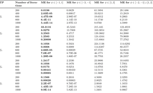
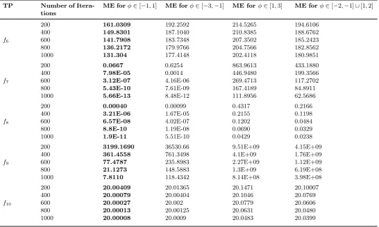
of parameter φ. From Table 2, it can be observed that the minimum mean error is obtained if φ∈[−1,1].

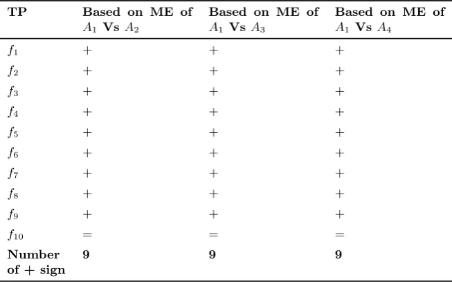
In order to check whether this difference in mean error is due to randomness or not, a non-parametric test, Mann-Whiteny U rank sum test is applied. In this study, the test is performed on mean error at 5% level of significance betweenABCwith stable range and ABC withφ∈[−3,−1], φ∈[−2,−1]∪[1,2] andφ∈[1,3]. Table 4 represents results of Mann-Whiteny U rank sum test for mean error (ME) over 100 runs.

Table 2

Mean Error(ME)for various ranges ofφ(TP: Test Problem)

TP Number of Itera-tions

ME forφ∈[−1,1] ME forφ∈[−3,−1] ME for φ∈[1,3] ME forφ∈[−2,−1]∪[1,2]

f1

200 0.0198 0.0829 61.5894 29.1486

400 2.03E-05 0.00017 33.0215 15.2819

600 4.47E-08 2.98E-07 19.6312 9.2063

800 6.4E-11 4.14E-10 14.1740 6.2110

1000 5.44E-14 2.97E-13 9.8760 4.5989

f2

200 33.3116 45.5243 215.445 123.4919

400 8.9279 13.7808 163.3054 95.2967

600 3.2563 6.4717 139.3662 84.2060

800 1.2583 3.2553 124.4344 79.9609

1000 0.20008 1.5042 115.8064 77.2762

f3

200 0.1056 0.5024 224.1136 114.6292

400 0.0008 0.0089 114.6387 80.2577

600 2.66E-05 0.00029 67.5725 52.8610

800 7.0E-07 8.79E-06 46.1771 35.7186

1000 1.29E-08 1.86E-07 33.7703 26.2357

f4

200 1.2417 2.2330 23.9806 10.8493

400 0.1056 0.1876 16.8943 7.7951

600 0.0173 0.0254 14.0703 6.8470

800 0.00441 0.00450 12.5115 6.3361

1000 0.00065 0.0011 11.5609 6.1795

f5

200 0.1566 0.2616 4.5688 2.3293

400 0.00020 0.00063 2.8025 1.4782

600 2.2E-07 8.76E-07 2.0048 1.1653

800 1.43E-10 7.28E-10 1.5822 1.0061

Table 2 Continued:

TP Number of Itera-tions

ME forφ∈[−1,1] ME forφ∈[−3,−1] ME for φ∈[1,3] ME forφ∈[−2,−1]∪[1,2]

f6

200 161.0309 192.2592 214.5265 194.6106

400 149.8301 187.1040 210.8385 188.6762

600 141.7908 183.7348 207.3502 185.2423

800 136.2172 179.9766 204.7566 182.8562

1000 131.304 177.4148 202.4118 180.9851

f7

200 0.0667 0.6254 863.9613 433.1880

400 7.98E-05 0.0014 446.9480 199.3566

600 3.12E-07 4.16E-06 269.4713 117.2702

800 5.43E-10 7.61E-09 167.4189 84.8911

1000 5.66E-13 8.48E-12 111.8956 62.5686

f8

200 0.00040 0.00099 0.4317 0.2166

400 3.21E-06 1.67E-05 0.2155 0.1198

600 6.57E-08 4.02E-07 0.1202 0.0484

800 8.8E-10 1.19E-08 0.0690 0.0329

1000 1.9E-11 5.51E-10 0.0429 0.0238

f9

200 3199.1690 36530.66 9.51E+09 4.15E+09

400 361.4558 761.3498 4.1E+09 1.76E+09

600 77.4787 235.8983 2.27E+09 1.12E+09

800 21.1273 148.5883 1.3E+09 6.19E+08

1000 7.8110 118.4342 8.14E+08 3.98E+08

f10

200 20.00409 20.01365 20.1471 20.10007

400 20.00079 20.00404 20.1046 20.0769

600 20.00027 20.002 20.0779 20.0606

800 20.00013 20.00125 20.0631 20.0480

Table 3

Comparision of ABC algorithm for various ranges ofφusing Mann-Whiteny U rank sum test (TP: Test Problem,ME: Mean Error,A1: φ∈[−1,1],A2: φ∈[−3,−1],A3: φ∈[1,3],A4: φ∈[−2,−1]∪[1,2] )

TP Based on ME of

A1 Vs A2

Based on ME of

A1 Vs A3

Based on ME of

A1 Vs A4

f1 + + +

f2 + + +

f3 + + +

f4 + + +

f5 + + +

f6 + + +

f7 + + +

f8 + + +

f9 + + +

f10 = = =

Number of + sign

9 9 9

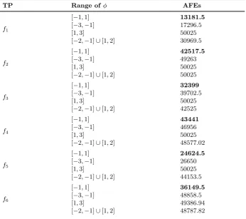
5.3

Efficiency

To see the effect of parameterφover the efficiency of ABC algorithm, numerical experiments are performed.

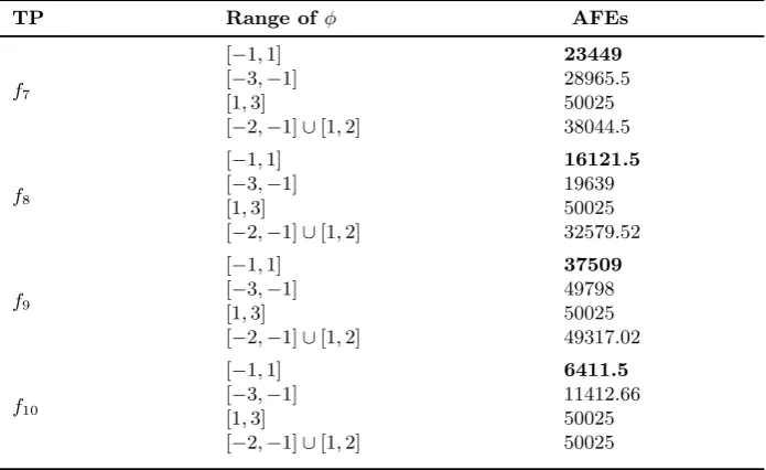
Table 4

AFEsfor various ranges ofφ(AFEs: Average number of Function Evaluations,TP: Test Problem)

TP Range ofφ AFEs

f1

[−1,1] 13181.5

[−3,−1] 17296.5

[1,3] 50025

[−2,−1]∪[1,2] 30969.5

f2

[−1,1] 42517.5

[−3,−1] 49263

[1,3] 50025

[−2,−1]∪[1,2] 50025

f3

[−1,1] 32399

[−3,−1] 39702.5

[1,3] 50025

[−2,−1]∪[1,2] 42525

f4

[−1,1] 43441

[−3,−1] 46956

[1,3] 50025

[−2,−1]∪[1,2] 48577.02

f5

[−1,1] 24624.5

[−3,−1] 26650

[1,3] 50025

[−2,−1]∪[1,2] 44153.5

f6

[−1,1] 36149.5

[−3,−1] 48858.5

[1,3] 49386.94

Table 4 Continued:

TP Range ofφ AFEs

f7

[−1,1] 23449

[−3,−1] 28965.5

[1,3] 50025

[−2,−1]∪[1,2] 38044.5

f8

[−1,1] 16121.5

[−3,−1] 19639

[1,3] 50025

[−2,−1]∪[1,2] 32579.52

f9

[−1,1] 37509

[−3,−1] 49798

[1,3] 50025

[−2,−1]∪[1,2] 49317.02

f10

[−1,1] 6411.5

[−3,−1] 11412.66

[1,3] 50025

[−2,−1]∪[1,2] 50025

As an overall observation, the performance of ABC algorithm significantly deteriorates if the range of parameter φ is deviated from the stable range [−1,1]. From above numerical experi-ments, we can say that for better convergence, accuracy and efficiency the recommended range of parameterφis same as the stable range [−1,1] obtained in section 4.

6

Conclusion and Future Work

Mathematical validity of parameters of probabilistic algorithms has always been a challenging task. Stability theory can help to derive value or the range of one or more parameters for the algorithms. In this paper, stability analysis of the ABC position update equation with parameter φand coefficientψhas been carried out. A generic method for testing the stability, von Neumann stability procedure for two-level finite difference scheme is considered. The outcome of stability analysis verifies the usual settings of parameter φ in the range [-1, 1]. Also stability condition depending on parameterφand coefficientψ is proposed which will bound the error in subsequent iterations. The findings are verified with graphical interpretation and numerical results over test problems. The study can also further be extended for the convergence analysis of ABC algorithm.

7

Acknowledgement

The second author acknowledges the funding from South Asian University New Delhi, India to carry out this research.

Appendix A

Finding amplification factor discussed in equation (18).

As discussed in section 3.3, amplification factor is calculated by replacing each termxn l of the

difference equation (15) by vn_(k)eι(kl∆i) _{and then using equation (16). After doing the required}

substitutions, equation (15) is modified as

vn+1(k)eι(kl∆i)= (ψ+φ)vn(k)eι(kl∆i)−(φ)vn(k)eι(k(l±a)∆i) (41)

or

vn+1(k) = (ψ+φ)vn(k)−(φ)vn(k)eι((±a)k∆i) (42)

or

vn+1(k) =

(ψ+φ)−(φ)eι((±a)k∆i)

By comparing equation (16) and (43), the amplification factor is given by

g(k) = (ψ+φ)−φeι(θ), where θ= ((±a)k∆i) (44)

Similarly, amplification factor described in equation (27) can be calculated.

Appendix B

Finding modulus of amplification factor discussed in equation (19).

By using equation (18), amplification factor is given by

g(k) = (ψ+φ)−φeι(θ) (45)

or

g(k) = (ψ+φ)−φ(cos(θ))−ιφsin(θ) (46)

By taking modulus of the above equation we get

|g(k)|=

q

(ψ+φ)−φcos(θ)2

+

φsin(θ)2

(47)

By further expansion, the above equation (47) is modified as

|g(k)|=

q

(ψ+φ)2+φcos(θ)2−2φ(ψ+φ)cos(θ) + (φsin(θ))2 (48)

or

|g(k)|=

q

(ψ+φ)2+φ2_{−2φ(ψ+φ) 1−2sin}2_(θ/2)

(49)

or

|g(k)|=

q

(ψ+φ)2+φ2_{−2φ(ψ+φ) + 4φ(ψ+φ)sin}2_{(θ/2) (50)}

or

|g(k)|=

q

(ψ+φ−φ)2+ 4φ(ψ+φ)sin2_{(θ/2) (51)}

or

|g(k)|=pψ2_{+ 4φ(ψ+φ)sin}2_{(θ/2) (52)}

Similarly, modulus of amplification factor given in equation (27) can be calculated.

References

References

[1] Ajith Abraham, Amit Konar, Nayan R Samal, and Swagatam Das. Stability analysis of the ant system dynamics with non-uniform pheromone deposition rules. InEvolutionary Computation, 2007. CEC 2007. IEEE Congress on, pages 1103–1108. IEEE, 2007.

[2] Bahriye Akay and Dervis Karaboga. Parameter tuning for the artificial bee colony algorithm.

ICCCI, 2009:608–619, 2009.

[3] Reza Akbari, Ramin Hedayatzadeh, Koorush Ziarati, and Bahareh Hassanizadeh. A multi-objective artificial bee colony algorithm. Swarm and Evolutionary Computation, 2:39–52, 2012.

[4] Bilal Alatas. Chaotic bee colony algorithms for global numerical optimization.Expert Systems with Applications, 37(8):5682–5687, 2010.

[5] DervisKaraboga BahriyeAkay. A modified abc algorithm for real parameter optimization.

information sciences, 192, 2012.

[7] Jagdish Chand Bansal, Harish Sharma, and Shimpi Singh Jadon. Artificial bee colony algo-rithm: a survey. International Journal of Advanced Intelligence Paradigms, 5(1-2):123–159, 2013.

[8] Adil Baykaso˘glu, Lale ¨Ozbakır, and Pınar Tapkan. Artificial bee colony algorithm and its ap-plication to generalized assignment problem. InSwarm intelligence, focus on ant and particle swarm optimization. InTech, 2007.

[9] Arijit Biswas, Swagatam Das, Ajith Abraham, and Sambarta Dasgupta. Stability analysis of the reproduction operator in bacterial foraging optimization. Theoretical Computer Science, 411(21):2127–2139, 2010.

[10] Swagatam Das, Subhodip Biswas, and Souvik Kundu. Synergizing fitness learning with

proximity-based food source selection in artificial bee colony algorithm for numerical opti-mization. Applied Soft Computing, 13(12):4676–4694, 2013.

[11] Swagatam Das, Sambarta Dasgupta, Arijit Biswas, Ajith Abraham, and Amit Konar. On stability of the chemotactic dynamics in bacterial-foraging optimization algorithm. IEEE Transactions on Systems, Man, and Cybernetics-Part A: Systems and Humans, 39(3):670– 679, 2009.

[12] Sambarta Dasgupta, Swagatam Das, Arijit Biswas, and Ajith Abraham. On stability and convergence of the population-dynamics in differential evolution.Ai Communications, 22(1):1– 20, 2009.

[13] ZH Ding, M Huang, and ZR Lu. Structural damage detection using artificial bee colony algorithm with hybrid search strategy. Swarm and Evolutionary Computation, 28:1–13, 2016.

[14] Amer Draa and Amira Bouaziz. An artificial bee colony algorithm for image contrast en-hancement. Swarm and Evolutionary computation, 16:69–84, 2014.

[15] Hai-bin Duan, Chun-fang Xu, and Zhi-Hui Xing. A hybrid artificial bee colony optimization and quantum evolutionary algorithm for continuous optimization problems. International Journal of Neural Systems, 20(01):39–50, 2010.

[16] Faezeh Farivar and Mahdi Aliyari Shoorehdeli. Stability analysis of particle dynamics in gravitational search optimization algorithm. Information Sciences, 337:25–43, 2016.

[17] Zong Woo Geem, Joong Hoon Kim, and GV Loganathan. A new heuristic optimization

algorithm: harmony search. Simulation, 76(2):60–68, 2001.

[18] Anshul Gopal and Jagdish Chand Bansal. Stability analysis of differential evolution. In

Computational Intelligence (IWCI), International Workshop on, pages 221–223. IEEE, 2016.

[19] Tsung-Jung Hsieh, Hsiao-Fen Hsiao, and Wei-Chang Yeh. Forecasting stock markets using wavelet transforms and recurrent neural networks: An integrated system based on artificial bee colony algorithm. Applied soft computing, 11(2):2510–2525, 2011.

[20] Visakan Kadirkamanathan, Kirusnapillai Selvarajah, and Peter J Fleming. Stability analysis of the particle dynamics in particle swarm optimizer. IEEE Transactions on Evolutionary Computation, 10(3):245–255, 2006.

[21] Dervis Karaboga. An idea based on honey bee swarm for numerical optimization. Technical report, Technical report-tr06, Erciyes university, engineering faculty, computer engineering department, 2005.

[22] Dervis Karaboga and Bahriye Akay. A modified artificial bee colony (abc) algorithm for constrained optimization problems. Applied soft computing, 11(3):3021–3031, 2011.

[23] Dervis Karaboga and Bahriye Basturk. Artificial bee colony (abc) optimization algorithm for solving constrained optimization problems. InInternational Fuzzy Systems Association World Congress, pages 789–798. Springer, 2007.

[25] Mina Husseinzadeh Kashan, Nasim Nahavandi, and Ali Husseinzadeh Kashan. Disabc: a new artificial bee colony algorithm for binary optimization. Applied Soft Computing, 12(1):342– 352, 2012.

[26] James Kennedy. Particle swarm optimization. In Encyclopedia of machine learning, pages 760–766. Springer, 2011.

[27] Mustafa Servet Kiran. The continuous artificial bee colony algorithm for binary optimization.

Applied Soft Computing, 33:15–23, 2015.

[28] Pravin Yallappa Kumbhar and Shoba Krishnan. Use of artificial bee colony (abc) algorithm in artificial neural network synthesis. Int J Adv Eng Sci Technol, 11(1):162–171, 2011.

[29] Guoqiang Li, Peifeng Niu, and Xingjun Xiao. Development and investigation of efficient artificial bee colony algorithm for numerical function optimization. Applied soft computing, 12(1):320–332, 2012.

[30] Ning Li, De-Bao Sun, Tong Zou, Yuan-Qing Qin, and Yu Wei. Analysis for a particle’s trajectory of pso based on difference equation.Jisuanji Xuebao/Chinese Journal of Computers, 29(11):2052–2061, 2006.

[31] Magdalena Metlicka and Donald Davendra. Chaos driven discrete artificial bee algorithm for location and assignment optimisation problems. Swarm and Evolutionary Computation, 25:15–28, 2015.

[32] Celal Ozturk and Dervis Karaboga. Hybrid artificial bee colony algorithm for neural network training. InEvolutionary Computation (CEC), 2011 IEEE Congress on, pages 84–88. IEEE, 2011.

[33] Esmat Rashedi, Hossein Nezamabadi-Pour, and Saeid Saryazdi. Gsa: a gravitational search algorithm. Information sciences, 179(13):2232–2248, 2009.

[34] Robert D Richtmyer and KW Morton. Different methods for initial value problems. Inter-science, 1967.

[35] Amani Saad, Salman A. Khan, and Amjad Mahmood. A multi-objective evolutionary artifi-cial bee colony algorithm for optimizing network topology design. Swarm and Evolutionary Computation, 2017.

[36] Nayan R Samal, Amit Konar, Swagatam Das, and Ajith Abraham. A closed loop stability analysis and parameter selection of the particle swarm optimization dynamics for faster conver-gence. InEvolutionary Computation, 2007. CEC 2007. IEEE Congress on, pages 1769–1776. IEEE, 2007.

[37] Rainer Storn and Kenneth Price. Differential evolution–a simple and efficient heuristic for global optimization over continuous spaces. Journal of global optimization, 11(4):341–359, 1997.

[38] Ioan Cristian Trelea. The particle swarm optimization algorithm: convergence analysis and parameter selection. Information processing letters, 85(6):317–325, 2003.