Cerebellar Models
M. D. Baxendale
1, M. J. Pearson
2, M. Nibouche
3, E. L. Secco
4, and A. G. Pipe
2Abstract
A robot audio localization system is presented that combines the outputs of multiple adaptive filter models of the Cerebellum to calibrate a robot’s audio map for various acoustic environments. The system is inspired by the MOdular Selection for Identification and Control (MOSAIC) framework. This study extends our previous work that used multiple cerebellar models to determine the acoustic environment in which a robot is operating. Here, the system selects a set of models and combines their outputs in proportion to the likelihood that each is responsible for calibrating the audio map as a robot moves between different acoustic environments, or contexts. The system was able to select an appropriate set of models, achieving a performance better than that of a single model trained in all contexts, including novel contexts, as well as a baseline GCC-PHAT sound source localization algorithm. The main contribution of this work is the combination of multiple calibrators to allow a robot operating in the field to adapt to a range of different acoustic environments. The best performances were observed where the presence of aResponsibility Predictorwas simulated.
I. INTRODUCTION
Audio can be used by autonomous mobile robots in unstructured environments when other senses, such as vision, break down. For example, in a disaster situation, where it is common to find high concentrations of airborne particles, vision could become impaired as the robot navigates the environment. The motivation for this study is for a robot to be able to locate an entity (such as a person in distress) based on the sounds it produces.
The proposed system uses models of cerebellar microzones [1], each of which has learned to calibrate the output of a robot’s Sound Source Localization (SSL) unit in a different environment, to select a set of models for each environment that the robot operates in. The approach is inspired by the MOdular Selection and Identification for Control (MOSAIC) framework [2], developed in the context of motor control in which aresponsibility estimatordetermines the degree to which each model is appropriate for the context, producing a set of posterior probabilities known asresponsibility signals. The system combines the outputs of the cerebellar calibration models in proportion to the responsibility signals. This study extends previous work in which cerebellar calibration of a distorted audio map was used with multiple models to determine a robot’s acoustic environment [3] and to calibrate the visual-tactile map of a whiskered robot [4]. Here, the models are combined in such a way as to improve calibration of the SSL output in different acoustic contexts. For the purposes of this study, a basic cross-correlation SSL algorithm was used. However, in principle, any SSL algorithm could be substituted for the one used, potentially improving robustness of the overall system to background noise, multiple sound sources and so on. The main contribution of this work, rather than demonstrating a robust SSL algorithm, is the demonstration that the combination of multiple cerebellar models allows a robot that has learned to calibrate SSL output in different environments, to select an appropriate set of models as it moves between the different acoustic environments, including, to a limited extent, novel environments.
II. BACKGROUND
A. Robot Audition and Sound Source Localization
Robot audition is a relatively recent area of research developing the ability for robots to listen [5], and is related to Computational Auditory Scene Analysis (CASA) [6]. According to Okuno et al. [7], robot audition consists of three key functions: SSL, sound source extraction (separation of the sound sources in the audio scene) and source recognition. SSL forms the focus of this work, which draws on robot audition, the adaptive filter model of the cerebellum and MOSAIC to calibrate SSL in different acoustic contexts. A number of attempts have been made to allow a robot to navigate by sound [8], [9], however these systems are typically set up in a specific acoustic environment and can break down if the robot moves to an unexplored environment. Practical SSL schemes typically utilise arrays of multiple microphones, e.g. [10], [11], [12], [13], however size, computation and power constraints on a mobile robot make the study of binaural techniques a compelling choice [14], and that is the approach used in this study. Binaural cues are reviewed in [15], and the two most commonly used are Inter-aural Time Difference (ITD) of arrival of sounds and Inter-aural Level Difference (ILD) [16]. ILD is effective at higher frequencies as it is based on the difference in intensity at the two sensors caused by frequency dependent scattering
1M. D. Baxendale is with the University of the West of England, Bristol, UK and Liverpool Hope University, Liverpool, UK.
[email protected], [email protected]
2M. J. Pearson and A. G. Pipe are with Bristol Robotics Laboratory, UK.[email protected], [email protected] 3M. Nibouche is with the University of the West of England, Bristol, UK.[email protected]
0o
Azimuth θ
90o
-90o
45o
-45o 90o
45o
0o
-90o -45o
Elevation α
θ α
Sound source
Robot head
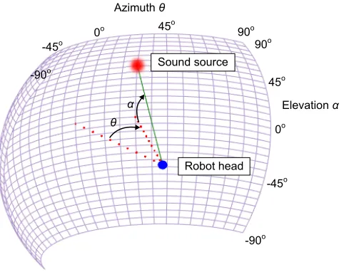
Fig. 1. Audio map of sound source location in head-centric space. The full map is a sphere centred on the robot head. The sound source location is a probabilistic position on the surface of the sphere at a fixed distance from the robot head. In this study, elevation is not considered, thereforeα=0. Radial distance is also fixed. Azimuthθis restricted to±45o.
by the head of the robot, whereas ITD is limited to lower frequencies as the period of the sound wave becomes comparable to the maximum ITD, giving rise to phase ambiguity [16]. This work focuses on ITD, with microphones mounted in free field, corresponding to Auditory Epipolar Geometry (AEG) [8], [5], and the Head Related Transfer Function (HRTF) is not considered. Sound from a source to either side of zero azimuthθ(see Fig. 1) will reach the sensors at different times. ITD is sensitive to environmental characteristics such as reverberation, which can result in distortion of the SSL estimate. In this study we consider SSL only in the azimuthal plane. Most binaural SSL systems have been tested under controlled, limited conditions [17], [18], [19], [20], [21]. A recent area of research related to CASA is Acoustic Scene Classification (ASC), which seeks to identify the acoustic environment from the audio stream [22], however limited work appears to have been carried out on how SSL systems can identify and adapt to different acoustic environments. This work aims to provide a means for SSL systems to be calibrated in various acoustic contexts. The robot head and SSL method are described more fully in section IV.
B. Cerebellar calibration of the audio map
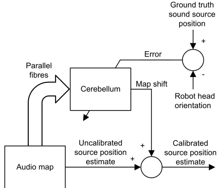
Cerebellar calibration of the audio map is based on the adaptive filter model of the cerebellum [1], [23], which has proven to be a robust algorithm in a variety of robotics applications [4], [24], [25]. The technique used here is described more fully in [3], and is adapted from [4]. The adaptive filter model of the cerebellum analyses input(s) into a number ofparallel fibres, which synapse onto the Purkinje Cell, which in turn forms the output of the adaptive filter. An error signal adapts the parallel fibre/Purkinje Cell weights (in the Cerebellum this is via the climbing fibres). In [4] a distinct visual marker attached to the target was used to determine the error in location estimation after the motor action. Here, we derive the error using the ground truth azimuth taken directly from the odometry of the test platform during the training of the different models (described in section IV). It is envisaged however, that a robot operating in the field could use vision to determine the error in localization during training of the models.
For audio calibration, shown in Fig. 2, parallel fibre input is activated by input from the underlying SSL unit and transmits a course coded, probabilistic representation of the estimated sound source azimuth as provided by the SSL unit.
The output of each model is the weighted sum of its inputs:
δθ=
n X
i=0
wipi (1)
wherenis the number of parallel fibres,pi the activity on theith parallel fibre andwi is the weight of the ith synapse. This
output represents a compensatory bias that is added to the SSL unit estimate, resulting in a calibrated estimate of sound source azimuth.
The weights wi are updated using the covariance learning rule [26], [4]:
∆wi=−βepi (2)
Fig. 2. Adaptive filter model of the cerebellum. Input to the filter is sound source position as coded in the audio map. Each parallel fibre represents activity at a number of sites on the map, so that the input is a course-coded version of the map.
+
+ Cerebellum Parallel
fibres
Ground truth sound source
position
Robot head orientation
+
-Error
Uncalibrated source position
estimate
Map shift
Audio map
Calibrated source position
estimate
Fig. 3. Cerebellar audio map calibration model in learning mode.
The cerebellar calibration model in learning mode is shown in Fig. 3. The error in sound source estimation (derived in this study using the platform odometry as mentioned earlier in this section) is used to train the model. Post learning, the cerebellar model is then able to apply a shift to compensate for SSL errors. As mentioned in section II-A, the system currently operates in 1 dimension, but could be extended to 2 dimensions (indeed, the work from which the system is adapted operated on a 2 dimensional whisker map [4]). Extension to 2 dimensions or even 3 would involve the same number of models, but with an increase in structural complexity.
C. Multiple models
A problem with a single model is that it would need to be highly complex to capture the range of contexts (acoustic environments) within which a robot operates in the field, or would need to adapt for each context. It has been proposed that the brain makes use of multiple models, each of which has learned to perform in a particular context [2]. A candidate approach to selecting models for a range of contexts is the MOSAIC framework [2], which was developed in the context of motor control but is re-purposed here for audio map calibration by adaptive filter models of the cerebellum. MOSAIC consists of an array of modules each of which could be responsible for control in a particular context. Each module consists of three main elements, a forward model, inverse model and Responsibility Predictor (RP). There is a separate responsibility estimator that operates across the modules. Inputs to the system are sensory feedback (of the consequences of action) and contextual signals. The forward models learn to predict the consequences of action in a particular context while the inverse models learn to control in the same context. The forward model’s prediction error is transformed into a likelihood that its module is responsible for control. At each point in time, all models make a prediction, and the prediction error of each is normalized across all modules, by the responsibility estimator, using a softmax function, to produce a responsibility signal for each module:
λi=
e−|xt−xi|2/σ2
Pn
j=1e−|xt−xj|
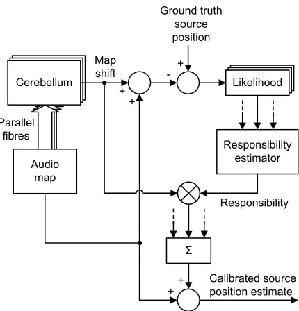
Fig. 4. Multiple-models- inspired audio localization as it has been implemented in this study. For a given context, each model generates a map shift that, when added to a copy of the output from the audio map, generates a prediction of source azimuth. The responsibility estimator produces a responsibility signal for each model, based on the posterior likelihood calculation. The overall map shift is produced from a summation of model map shifts in proportion to their responsibility.
where xt is the true value of the next state of the system,xi is the estimate produced by theith model, n is the number of
estimates (models) and σ is a scaling factor. The responsibility signal is used to modulate the output of the module, before summing outputs across modules to produce an overall output. The likelihoods are posterior in that they cannot be determined until after action has taken place, which may lead to transient performance errors when the context changes, and the RP in MOSAIC uses contextual signals to produce a prior prediction of the responsibility signals. The number of models is equal to the number of contexts that the robot has experienced and learned in. However, a claim of the MOSAIC framework is that it should be possible for the system to generalize to novel contexts that are characterized by features that fall intermediate to those of the contexts in which each model has been specifically trained. This means that the robot should be able to cope with more contexts than the number of models it possesses.
III. PROPOSED SYSTEM
The system developed in this study is shown in Fig. 4. It is MOSAIC-inspired rather than being a faithful reproduction of the framework. Rather than MOSAIC’s forward/inverse model pair, the proposed system has a single model that is used for both prediction of the sound source position and calibration of the audio map. The system also implements MOSAIC’s responsibility estimator, the outputs of which are used to modulate the outputs of the model. The system has a single ITD based SSL unit that produces an estimate of sound source azimuth using a cross-correlation algorithm (see section IV-B). Each cerebellar model, having been trained in a particular context (section IV-C), produces a map-shift signal based on the output of the SSL unit and each shift is individually added to the SSL unit output to form the prediction for each model. Each model prediction is compared to the ground truth position of the sound source.
Each model’s prediction error is transformed and normalized across all models as in the MOSAIC framework using an adaptation of equation 3:
λi=
e−|θt−θi|2/σ2
Pn
j=1e−|θt−θj|
2/σ2 (4)
where θt is the ground truth azimuth and θi is the estimate produced by the ith model. As explained in section II-B, in
the experiments described here, θt is derived directly from the odometry, whilst in the field a robot would find θt through
sensory feedback, as in MOSAIC, via another modality such as vision. The ground truth may not always be available to a robot operating in the field (e.g. through obscured vision), and it is assumed that a robot operating in the field would use the most recently available ground truth value to compute the responsibility signals. The modulated model outputs are summed to produce an overall map shift, with a contribution from each model in proportion to its responsibility signal.
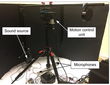
Motion control unit Sound source
Microphones
Fig. 5. Photograph of the experimental arena. A motion control unit (Dynamic Perception Stage R) powered by a stepper motor is mounted on a tripod such that it is centered on the robot head vertical axis. A horizontal beam attached to the motion control unit allows the sound source to be placed at various azimuths with respect to the robot head.
λi =
λpie−|θt−θi|
2/σ2
Pn
j=1λpje−|θt−θj|
2/σ2 (5)
whereλpi is the predicted value of the responsibility of theith model. In the field, this would allow the responsibility to be
updated even before the robot were to orient toward the sound source, based on features extracted from the audio stream. The RP is simulated here and an implementation is the subject of future work.
IV. METHOD
A. Experimental setup
Matlab (The Mathworks Inc.) was used to control experiments and for implementation of algorithms. Two microphones (Audio-Technica ATR-3350 omnidirectional condenser lavalier) were mounted in free field at the extremities of a horizontal bar (Fig. 6), with an inter-microphone distance of 0.25m and were connected to a computer using a M-Audio MobilePre USB audio capture unit. A sampling rate of 44100Hz was used. Sound pressure level at the microphones was measured using a Max Measure MM-SMB01 sound level meter and was maintained at approximately 70dBA with the sound source directly facing the robot head. Background noise was present in all experiments including acoustic noise generated by the PTU, even while the motion control system was stationary.
A sound source (Logitech Z150 Speaker) was positioned at a fixed distance from the robot head (Fig. 5) and was connected to the computer sound card. Short distances were used due to experimental constraints (0.4m-1m). Although this potentially violates the far field assumption made in this work, localization has been successfully carried out at comparable distances [27], also any violation should be constant across conditions for comparison purposes. Different acoustic contexts were created by rotating the sound source on its vertical axis using a stepper motor under computer control such that it could face away from the robot head at an angleφas shown in Fig. 7. The sound source/stepper motor assembly was suspended from a beam which itself was mounted on a tripod whose central column was placed over the robot head. A geared stepper motor was used to rotate the beam, using a motion control platform (Dynamic Perception Stage R) such that the sound source could be placed in robot-head centric space under computer control at any azimuth between -45o (left with respect to the robot head) and +45o.
B. SSL unit
The SSL unit used a cross-correlation algorithm to generate an estimate of the azimuthal position of a sound source:
rlr = n X
k=0
R(k)L(k−τ) (6)
whereRis the right- andLthe left channel audio signal,kis the sample number,nis the number of samples andτis the time lag between audio channels. The ITD value corresponds to the time difference that results in maximum similarity between the two channels. The estimated azimuthal position can be calculated from the ITD value as:
θ= 180
π sin
−1(cτ dfs
) (7)
Microphones
Fig. 6. Close-up photograph of the robot head. The head is mounted on a pan-and-tilt unit (eMotimo TB3) that allows the centrally mounted camera to be oriented toward the estimated sound source position to ascertain ground truth, although this was not used in this study. Microphones were mounted in free field at either end of the bar.
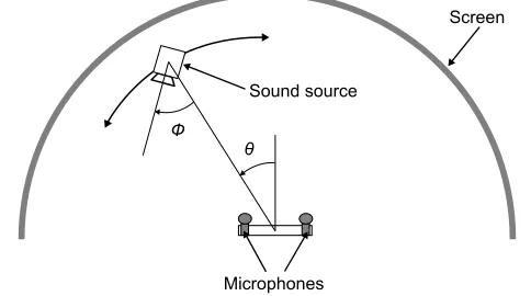
Screen
Sound source
θ Ф
Microphones
Fig. 7. Plan view of the experimental arena. The sound source was oriented at a fixed angle (φ) on its vertical axis in each context, and placed at various azimuths (θ).
C. Cerebellar models
Each cerebellar model was trained in one acoustic context with the sound source facing at a different angle (φin Fig. 7) for each context (90o left; 0o and 90o right with respect to the robot head). During learning, the robot head was presented with audio (a 1 second duration Gaussian noise signal) from randomized directions (θin Fig. 7). After training, the robot head was presented with a sequence of audio stimuli in different contexts, with 5 stimuli per context having randomized sound source azimuth. The values ofφwere chosen as multiples of the resolution of the sound-source mounting stepper motor, 1.8o. Audio stimuli were generated at 1oincrements and recorded for off-line training and testing of the system. In the first two experiments (section V-B and V-D), the same 3 contexts were used that the models were trained in. In the third experiment (section V-F), 2 novel contexts were used with values of φthat lay between those in which the models were trained. Responsibility signals were initialized to be uniformly equal at the start of each experimental run. The value of σin equations 4 and 5 was tuned by hand as in [2].
V. RESULTS
A. Overview
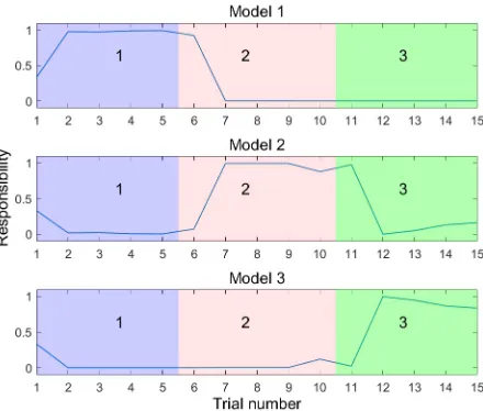
Fig. 8. Responsibility signals as the system progresses through the trials. In each trial the system is presented with stimulus of various azimuths in three different contexts, indicated by the coloured regions, labelled with the context number. Context 1 (blue region) isφ=90o left; context 2 (red region) isφ=0o;
context 3 (green region) isφ=90o right.
Fig. 9. Responsibility signals with a simulation of the presence of a responsibility predictor. In each trial the system is presented with stimulus of various azimuths in three different contexts, indicated by the coloured regions, labeled with the context number. Context 1 (blue region) isφ=90oleft; context 2 (red
region) isφ=0o; context 3 (green region) isφ=90o right.
frequency (44100Hz in this study) and inter-microphone distance (0.25m in this study). In all experiments the scaling factor
σ in equation 4 was set to a value of 2 (chosen so as to result in a low performance error over a large number of trials in learned contexts). Localization performance figures were calculated from 10 runs of each experiment of 15 trials.
B. Performance in learned contexts
TABLE I
LOCALIZATION PERFORMANCE. N=150. ACCURACY RATE IS PERCENT LESS THAN5O
ABSOLUTE ERROR
Method Accuracy
rate
MSE (degrees2)
1. Single model trained in all contexts 79% 13.5
2. GCC-PHAT 77% 13.6
3. Combined models 92% 5.8
4. Combined models with redundant models 92% 5.8 5. Combined models with RP 100% 1.5 6. Combined models, missing ground truth 91% 6.4 7. Missing ground truth, with RP 99% 2.4 8. Single model trained in novel contexts 88% 11.8 9. GCC-PHAT in novel contexts 86% 10.9 10. Combined models in novel contexts 91% 8.8 11. Single model in domestic contexts 33% 60.0 12. GCC-PHAT in domestic contexts 53% 64.0 13. Combined models in domestic contexts 76% 22.1
Fig. 10. Responsibility signals during trials in which additional models were present that had not been trained in the presented contexts. Models 1, 3, 5 and 7 had been trained in contexts in whichφwas set to 135o left, 45o left, 45o right and 135o right respectively. Models 2, 4 and 6 had been trained in the contexts presented (corresponding to models 1, 2 and 3 respectively in experiment V-B).
C. Performance in learned contexts with redundant models
As mentioned in section II-C, there would normally be one model per context, but there is a question of how well the system would perform if operating in a subset of the learned contexts, i.e., there were more models operating than required for the currently experienced sequence of contexts. The experiment was repeated with 7 models: the 3 used already plus models trained in contexts with values of φ of 135o left, 45o left, 45o right and 135o right. It can be seen from figure 10 that the models trained in the 3 presented contexts (models 2, 4 and 6) still dominated, with some sharing of responsibility with the additional models, but that the system has a comparable performance to that where only the trained models were present (row 4 of Table I).
D. Responsibility prediction
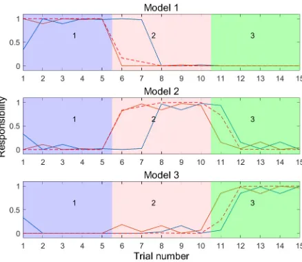
Fig. 11. Responsibility signals during trials in which the ground truth becomes unavailable in one of the trials (trial 6). In each trial the system is presented with stimulus of various azimuths in three different contexts, indicated by the coloured regions, labelled with the context number. Context 1 (blue region) is φ=90oleft; context 2 (red region) isφ=0o; context 3 (green region) isφ=90oright. The blue curve shows the output of the responsibility estimator, the orange
curve shows the output of the simulated responsibility predictor, and the red broken curve shows the overall responsibility calculated according to Equation 5.
results of this simulation are shown in Fig. 9, where earlier switching of responsibility can be observed between contexts. The localization performance (Table I row 5) is improved. Although the accuracy rate appears excellent, an implementation of the PR may not provide such good results.
E. Performance where the ground truth becomes unavailable
As mentioned in section III the ground truth may not always be available. The ground truth was made unavailable during one trial (trial 6). Fig. 11 shows plots of the responsibility signals of each model (blue curves). In this case the dominance of model 1 is extended into context 2, where dominance of model 2 would have been expected. This extension of the dominant model’s responsibility did not always happen; depending on the value of the SSL output, sometimes dominance of the responsibility switched temporarily to an altogether different model. In this experiment, the ground truth becomes available again during trial 7, and the system adjusts the responsibilities accordingly. Row 6 of Table I shows that the performance with this missing ground truth value has deteriorated slightly (we would expect more pronounced deterioration with prolonged absence of the ground truth). The RP potentially plays an important role in such situations, since an actual implementation of the RP would continue to receive contextual signals from the audio stream, even when the ground truth is unavailable. Plots of the RP output are also shown in Fig. 11 (orange curves), and the overall responsibility (broken red curves), calculated using equation 5, shows that the presence of a simulated RP causes more appropriate switching of the responsibilities. Row 7 of Table I shows that the poorer performance is mitigated to an extent by the presence of the RP.
F. Performance in novel contexts
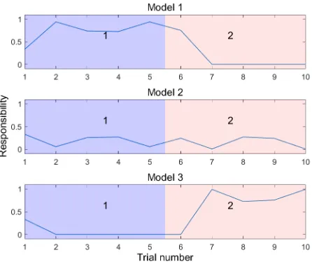
As described in section II-C, a claim of the MOSAIC framework is that combining the outputs of modules that have learned existing behaviours allows the generation of new behaviours to deal with new contexts. By analogy, the system proposed here ought to be able to combine existing cerebellar calibration to new, but similar contexts, by presenting the robot head with acoustic contexts that are intermediate to the ones in which the models were learned. The robot head was presented with contexts corresponding to sound source angles (φin Fig. 7) of 72o left; and 72o right with respect to the robot head. Figure 12 shows plots of the responsibilities as the system progressed through the trials in the two contexts. It can be seen that the models that have learned in contexts closest in characteristics to the novel contexts (models 1 and 3) tend to dominate, but less distinctly than in figure 8, so that there is more sharing between adjacent models. Rows 8- 10 of Table I show that the performance is better than a single model that was trained in the 3 previous contexts, and is similar to that of the GCC-PHAT SSL method.
G. Performance in domestic contexts
Fig. 12. Responsibility signals during trials in which novel contexts are presented. Plots show the responsibility of each model. In each trial the system is presented with stimulus of various azimuths in two different contexts, indicated by the coloured regions, labeled with the context number. Context 1 (blue region) isφ=72o left; context 2 (red region) isφ=72oright.
room, with a distance to source of 1m and sound source angle φset to 90o right. In the second context, the experiment was conducted in the corner of the room, with a distance to source of 0.5m and φset to 135o left. Performance was poorer than in previous experiments, however the proposed system still outperformed the single model trained in all contexts as well as the GCC-PHAT algorithm (rows 11- 13 of Table I).
VI. DISCUSSION AND FUTURE WORK
We have presented a multiple-models-inspired cerebellar calibration system for an audio map which was able to automatically select an appropriate set of models and combine the outputs of those models to calibrate the robot’s audio map in different acoustic contexts. The performance of the combined models was better than that of a single model trained in all contexts, as well as the baseline GCC-PHAT SSL algorithm, in both novel contexts and contexts in which the models had been trained. Including the simulation of a responsibility predictor further increases the performance by providing a prior prediction of responsibility, especially during transitions between contexts. However, an implementation of the RP may not behave in the same way, especially for novel contexts, and this is the subject of future work. The current study is restricted to SSL in 1 dimension, however, as mentioned in section II-B, we are confident the approach can scale up to 2 dimensions and this is a potential area of future work. In the current study, models are pre-trained, whereas a robot operating in the field will need to adapt to partly and completely novel acoustic contexts, and so future work will also include the investigation of adaptation and tabula rasa learning of the models, as described in [29].
REFERENCES
[1] P. Dean, J. Porrill, C. F. Ekerot, and H. Jorntell, “The cerebellar microcircuit as an adaptive filter: experimental and computational evidenc (report)”, Nature Reviews Neuroscience, vol. 11, no. 1, p. 30, 2010.
[2] D. M. Wolpert and M. Kawato, “Multiple paired forward and inverse models for motor control”, Neural Networks, vol. 11, no. 78, pp. 1317–1329, 1998. [3] M. D. Baxendale, M. J. Pearson, M. Nibouche, E. L. Secco, and A. G. Pipe, “Self-adaptive context aware audio localization for robots using parallel cerebellar models”, in Towards Autonomous Robotic Systems: 18th Annual Conference, TAROS 2017, Guildford, UK, 2017, Proceedings, Y. Gao, S. Fallah, Y. Jin, and C. Lekakou, Eds. Cham: Springer International Publishing, 2017, pp. 66–78.
[4] T. Assaf, E. D. Wilson, S. Anderson, P. Dean, J. Porrill, and M. J. Pearson, “Visual-tactile sensory map calibration of a biomimetic whiskered robot”, in 2016 IEEE International Conference on Robotics and Automation (ICRA). IEEE, 2016, Conference Proceedings, pp. 967–972.
[5] K. Nakadai, T. Lourens, H. Okuno and H. Kitano, “Active audition for humanoid”, in Proceedings of 17th National Conference on Artificial Intelligence (AAAI-2000) (2000), AAAI, pp. 832–839, 2000.
[6] H. G. Okuno, T. Ogata, K. Komatani, and K. Nakadai, “Computational auditory scene analysis and its application to robot audition”, International Conference on Informatics Research for Development of Knowledge Society Infrastructure, 2004, pp. 73–80, 2004.
[7] H. G. Okuno, K. Nakadai, “Robot audition: Its rise and perspectives”, 2015 IEEE International Conference on Acoustics, Speech and Signal Processing (ICASSP) 2015, pp. 5610–5614, 2015.
[8] S. Argentieri, P. Dan`es and P. Sou`eres, “A survey on sound source localization in robotics: From binaural to array processing methods”, in Computer Speech & Language, vol. 34, no. 1, pp. 87–112, 2015.
[9] C. Rascon, and I. Meza, “Localization of sound sources in robotics: A review”, Robotics and Autonomous Systems, vol. 96, pp. 184–210, 2017. [10] A. Badali, J. M. Valin, F. Michaud, P. Aarabi, “Evaluating real-time audio localization algorithms for artificial audition in robotics”, 2009 IEEE/RSJ
International Conference on Intelligent Robots and Systems (IROS), pp. 2033–2038, 2009.
[11] X. Li, M. Shen, W. Wang, H. Liu, “Real-time Sound Source Localization for a Mobile Robot Based on the Guided Spectral-Temporal Position Method”, International Journal of Advanced Robotic Systems, vol. 9, no. 78, 2012.
[15] K. Youssef, S.Argentieri, and J. L. Zarader, “Towards a systematic study of binaural cues”, 2012 IEEE/RSJ International Conference on Intelligent Robots and Systems, pp. 1004–1009, 2012.
[16] J. Blauert, Spatial hearing: the psychophysics of human sound localization, Cambridge, Mass; London; MIT Press, 1997, vol. Rev.
[17] V. Chan, C. Jin, and A. van Schaik, “Neuromorphic audio-visual sensor fusion on a sound-localizing robot”, Frontiers in Neuroscience, vol. 6, 2012. [18] J. Davila-Chacon, S. Magg, L. Jindong, and S. Wermter, “Neural and statistical processing of spatial cues for sound source localisation”, Neural Networks
(IJCNN), The 2013 International Joint Conference on, pp. 1–8, 2013.
[19] J. Huo and A. Murray, “The adaptation of visual and auditory integration in the barn owl superior colliculus with Spike Timing Dependent Plasticity”, Neural Networks, vol. 22, no. 7, 2009.
[20] J. A. Wall, T. M. McGinnity and L. P. Maguire, “A comparison of sound localisation techniques using cross-correlation and spiking neural networks for mobile robotics”, Neural Networks (IJCNN), The 2011 International Joint Conference on, pp. 1981–1987, 2011.
[21] K. Youssef, S.Argentieri, and J. L. Zarader, “A binaural sound source localization method using auditive cues and vision”, Neural Networks (IJCNN), Acoustics, Speech and Signal Processing (ICASSP), 2012 IEEE International Conference on, pp. 217–220, 2012.
[22] D. Barchiesi, D. Giannoulis, D. Stowell, and M. D. Plumbley, “Acoustic Scene Classification: Classifying environments from the sounds they produce”, IEEE Signal Processing Magazine, vol. 32, no. 3, pp. 16–34, 2015.
[23] M. Fujita, “Adaptive filter model of the cerebellum”, Biol Cybern, vol. 45, no. 3, pp. 195–206, 1982.
[24] J. Porrill, P. Dean, and S. R. Anderson, “Adaptive filters and internal models: Multilevel description of cerebellar function”, Neural Networks, vol. 47, pp. 134–149, 2013.
[25] J. Porrill, P. Dean, and J. V. Stone, “Recurrent cerebellar architecture solves the motor-error problem”, Proceedings of the Royal Society B: Biological Sciences, vol. 271, no. 1541, pp. 789–796, 2004.
[26] T. J. Sejnowski, “Storing covariance with nonlinearly interacting neurons”, J Math Biol, vol. 4, no. 4, pp. 303–21, 1977.
[27] H.-D. Kim, J.-S. Choi, M. Kim, Munsang and C.-H. Lee, “Reliable detection of sound’s direction for human robot interaction”, IEEE/RSJ International Conference on Intelligent Robots and Systems (IROS), vol. 3, pp. 2411–2416, 2004.
[28] C. Knapp and G. Carter, “The generalized correlation method for estimation of time delay”, IEEE Transactions on Acoustics, Speech, and Signal Processing, vol. 24, pp. 320-327, 1976.