Article
High spatial resolution climate scenarios to analyze
Madrid building energy demand
Roberto San José 1,*, Juan Luis Pérez 1 and Rosa Maria Gonzalez Barras 2
1 Software and Modelling Group, Computer Science School, Technical University of Madrid (UPM), Madrid, Spain ; [email protected]
2 Department of Physics and Meteorology, Faculty of Physics, Complutense University of Madrid (UCM), Ciudad Universitaria, 28040 Madrid, Spain
* Correspondence: [email protected]
Abstract: We have modelled the energy consumption of prototype and real buildings under present and future climatic conditions with the EnergyPlus model to develop a better understanding of the relationship between changing climate conditions and energy demand. We have produced detailed meteorological information with 50 meters of spatial resolution through dynamical downscaling process combining regional, urban and computational fluid dynamics models which include the effects of the buildings on urban wind patterns. The city of Madrid has been chosen for our experiment. The impact on energy demand and their respective economic cost are calculated for year 2100 versus 2011 based on two IPCC climate scenarios, RCP 4.5 (stabilization of emissions) and RCP 8.5 (not reduction of emissions). Findings show that climate change will have a significant impact on the energy demand for buildings. Space heating demand will be increased by the RCP 4.5 and cooling demand will be increased for the RCP 8.5 in the analysed buildings.
Keywords: climate; downscaling; impact; building
1. Introduction
Energy consumption for heating, ventilation and air conditioning (HVAC) has increased in recent years throughout Europe, especially in the South. In most countries of the European Union, a large part of the final energy consumption of buildings is used for heating and cooling. Under climate change these energy use patterns can change because climate variations affect the indoor environment of buildings and comfort levels [1]. Buildings designed according to past climatic conditions can be increasingly costly to operate and maintain in the present and future [2]. The energy demand for heating and cooling of building spaces is sensitive to climatic variables such as solar radiation, outdoor air temperature, wind, humidity, etc. It is then logical that the energy demand of buildings will be affected by climate change. Warmer or colder periods can reduce or increase the demand for heating and cooling in buildings. In addition, cities are the areas where the local response to global climate change is most pronounced [3]. Recent studies have suggested that global climate change will have a significant impact on local climate [4]. Understanding how climate change can affect the energy demand for buildings is essential for designing adaptation policies, which aim to minimize the adverse effects of climate change and exploit the potential benefits.
Demand for heating and cooling, fluctuates hourly, daily, and seasonally in response to outdoor meteorological conditions. As mentioned above, energy demand is determined by a number of meteorological factors. Some studies only focus on temperature in terms of heating degree days (HDDs) and cooling degree days (CDDs). However other factors influence the energy demand of buildings, such as humidity, wind, thermal comfort configuration and thermal characteristics of the building [5], so more sophisticated energy demand modelling systems are needed that include
complete weather simulations with the modelling of all atmospheric processes. Typically, analyses of the energy consumption of buildings are based on climate data from the current year or past years. However, there is a lack of analysis of the implications of future IPCC climate scenarios on the energy performance of buildings.
Therefore, we need several steps to achieve an integrated modeling of climate impacts on the energy demand of buildings. Firstly, we have to select a set of future climate scenarios; secondly we have to produce high-resolution meteorological data sets from global circulation models that are decreasing in scale using regional and urban climate models. In a third stage, meteorological variables are used to calculate direct effects on energy demand using the energy model.
In energy simulations of buildings, it is common to use regional meteorological data that are generally based on current or past weather conditions. However, most buildings have a lifetime of several decades, during which time the climate can change gradually. Therefore, energy simulations should incorporate future climate change predictions with high spatial resolution [6]. The atmospheric flow and special microclimate of cities are influenced by the characteristics of the urban surface [7]. Global climate models (GMCs) have a spatial resolution of about one degree, which can predict long-term climate trends, but their very coarse grid resolution (~100 km) cannot describe the details of local phenomena, so it is necessary to use higher resolution horizontal numerical models to obtain accurate data on the urban microclimate, taking into account all its special characteristics [8], so they must be carried out at a fine scale. The objective of downscaling is to bridge the spatial gaps in datasets between climate information predicted by global climate models and regional or urban climate information needed for other applications, such as this paper.
The downscaling can be done by two methods: the statistical downscaling (SD) or the dynamic downscaling (DD). In statistical downscaling, statistical relationships derived from regional data are used to scale down climate data on a large scale, so this method requires regional observations. When this method is used to predict future regional climate, an important question is whether the relationship derived from current data can be applied to future conditions influenced by global warming. To solve this problem, we use a dynamic downscaling method. In dynamical downscaling, global climate model data is entered as initial and boundary conditions to a Regional Climate Model (RCM); regional climate model analysis is used to physically scale down the global climate model data. Regional climate model uses nested regional climate models, and can analyze the local climate in high resolution (~1 km) [9]. Additionally, a computational fluid dynamics model can be used for very high resolutions (meters), in our case we have scaled down to 50 meters, taking into account the effects of buildings on the urban meteorological conditions.
The first studies on building cooling and heating demand were based on simplified analyses using constant annual mean temperature increases or changes in cooling degree-days and heating degree-days as discussed above. These results are insufficient in detail and may therefore be inaccurate in describing the impacts of climate change on energy demand in buildings. Recent improvements in global and regional climate modelling can improve detailed energy simulations of buildings and thus be able to study the impact of climate change in much more detail.
considerable impacts on energy use in buildings. These studies are regionally based and focus only on a few types of buildings, so the overall situation could not be predicted. Impact studies on future energy demands have a high uncertainty derived from uncertainties in the methods for projecting future climatic conditions [16].
In this study we investigate the potential impact of future climate change scenarios on heating and cooling energy demand to understand how building performance may vary in the future and help design effective adaptation strategies. Specifically, a dynamic scale reduction method is used to obtain future standard meteorological data at a local scale, specifically in this study is calculated at 50 meters spatial resolution, taking into account the shape of buildings, modeled as 3D structures and their effects on ventilation. This high-quality climate information is used to simulate the energy performance of buildings in future climate change scenarios. This report did not attempt to assess the climate impacts on the energy demand by droughts and the resulting changes in water availability, extreme precipitation events, flooding, or sea-level rise. Nevertheless the building energy simulations with projected future climate data may be useful first step to design effective adaptation strategies. Planners are already beginning to acknowledge the need to update energy demand and supply forecasts with climate data that are consistent with the IPCC climate scenarios. Our analysis shows significant changes in the heating and cooling demands of buildings under future climate scenarios (2100) compared to the 2011 reference year. The methodology described in the next section can be applied to any city buildings, if sufficient input data are available. The results presented are specific to the city of Madrid and they should be considered as an example of the application of the tool proposed in the paper.
2. Materials and Methods
To assess the impact of climate change on energy demand, the first step is to take a set of climate scenarios as a context. The impacts of climate change on energy consumption in buildings have been analysed for two Representative Concentrations Pathways (RCPs) [17], RCP 4.5 and RCP 8.5. These climate scenarios are currently being used in simulations of global climate models from the IPCC (Intergovernmental Panel on Climate Change) scenarios based on the Fifth Assessment Report (AR5) [18]. The IPCC report identifies up to four climate scenarios, ranging from very strong (unrealistic) mitigation scenarios (RCP 2.6) to a business-as-usual scenario (RCP 8.5). The choice of the worst-case scenario (RCP 8.5) and the best realistic scenario (RCP 4.5) was motivated by the objective of showing extreme changes that can be predicted on an urban scale and helping to implement mitigation and adaptation strategies. The RCP 8.5 scenario [19] is based on a small effort to reduce emissions and represents a failure to curb warming in 2100. It is characterised by increased greenhouse gas emissions over time. RCP 4.5 is a stabilisation scenario in which total radiative forcing is stabilised by 2050 using a range of technologies and strategies to reduce greenhouse gas emissions. This scenario can be seen as a climate change mitigation scenario [20]. Scenario RCP 4.5 implements strategies to reduce GHGs that will result in stabilization of radiative forcing at 4.5 W/m² by 2100, while RCP 8.5 assumes that radiative forcing can reach 8.5 W/m² by 2100.
Energy simulations of buildings require hourly climate data files to calculate the amount of energy consumed based on local conditions; in particular, data are needed for the following climatic variables: dry bulb temperature, wet bulb temperature, solar radiation, wind speed, wind direction, humidity and pressure. We need to generate 8760 values of these variables each year. Meteorological data is used not only to determine a building's energy response to the climate, but also to dimension the building's air conditioning systems. We have dynamically downscaled the Global Climate Model (GCM) outputs through a regional/urban climate model (RCM) and a computational fluid dynamics model (CFD) to resolutions of 50 meters. In this research we use the results of CESM as a GCM model, WRF as RCM and MICROSY as a CFD model, as explained below.
(CFD) model called MICROSYS [24] which operates at high spatial resolution (meters). This downscaling procedure was performed using boundary and initial condition data from the mother levels to the nested levels. The WRF model dynamically downscaled CESM global model data from 50 km spatial resolution to 1 km. The WRF operates through different spatial scales (50 km, 5 km, 1 km) using a domain nesting procedure. WRF outputs with UCM [25] (urban canopy model) at 1 km resolution were introduced (offline) in MICROSYS to initialize simulations and provide boundary conditions. The UCM model is based on the city's energy budget approach. The UCM model adopts the turbulent flow resistance net approach in the canyon. It takes into account recirculation and ventilation of air for calculation of turbulent heat flow within the canyon. Shading is represented in terms of sky view factors that represent the area of each urban surface and the sky that is visible by other urban surfaces (e. g. walls and roads). The UCM model is coupled to the WRF model at each step in which the stationary physical equations are solved. The exchange radiation, sensible heat, latent heat and moment fluxes are calculated by the UCM model and are coupled to the parameterisation of the turbulence shut-off limit layer of the WRF model. The MICROSYS CFD model is based on the MIMO CFD model (developed at the University of Karlsruhe), which takes into account building obstacles. The model includes a three-dimensional stable-state system of Reynolds equations, a k-ε and the "advection-diffusion" equation to simulate online transport. Surface energy flows have been implemented in the MICROSYS code based on the procedures applied in the UCM model and the NOAA Land-surface model included in the WRF modeling system. A SHAMO micro shadow model (developed by UPM) has been executed to calculate shade areas (including reflections on vertical walls of buildings) and short-wave radiation in high spatial resolution domains (some few meters). The 50-meter resolution allows each building block to have its own meteorological data sets. Meteorological data is calculated as the spatial average of the 50-meter grid cells around the building block. The description of the dynamic downscaling method has already been published in other papers, for details see publication [26]. We have produced climate data per hour with very high spatial resolution, data for each grid of 50 meters by 50 meters over the city of Madrid for 2011 (base year) and 2100 year (future year) for the climatic scenarios RCP 4.5 and RCP 8.5.
The energy demand for buildings is modeled by EnergyPlus [27]. It is a well-known and accepted tool in the energy analysis of community building worldwide and the model is highly validated. Taking into account the local climate of each building, EnergyPlus calculated the HVAC energy demand per hour of buildings to meet the thermal comfort of occupants for one year. EnergyPlus is based on complex calculations of heat gain and loss, including different physical processes such as transient heat conduction through the building envelope elements. It also performs heat and mass transfer by impacting sensitive and latent heat loads due to ventilation and infiltration. In addition, the model calculates detailed heat transfer from integrated solar gain models through filtration and surrounding soil components. The building model is based on the fundamental principles of thermal equilibrium. It assumptions that the air in the thermal zone, by default, has a uniform temperature, the temperature of each surface is uniform, the long and short wave radiation is uniform irradiation of the surface is diffuse and the conduction of heat through the surfaces is unidimensional. Simulations are carried out during one year periods with one hour climate update intervals. The heating and cooling demands are calculated by the EnergyPlus model. The model uses a submodule for Outside Surface Heat Balance (external thermal loads) and other for Inside Surface Heat Balance (internal thermal loads) and the internal and external thermal loads are connected by the Wall Surface Heat Balance (conduction into wall and conduction from outside). In this study, the internal thermal factors are the same in the present and in the future because we want to isolate the climate impacts (more information about these considerations are explained in the next paragraph). The external thermal loads are influenced by the climatic conditions and they will modify the internal thermal loads thank you to the conduction throw the wall of the buildings, so if we want to maintain the same thermal comfort inside the building, the energy demand will be different
ASHRAE 90.1 (PNNL 2014) prototype building modeling specifications developed by the Pacific Northwest National Laboratory (PNNL). Buildings are not supposed to change for future simulations (2100) to isolate the effects of global climate on the energy demand of buildings; the only changed input is the climate conditions. We isolate the climate impacts from other drivers that are expected to affect the building energy systems (e.g., thermal efficiency, expected socio-economic changes, policy and price effects) by comparing future climate pathways (2100) to a present scenario (2011). The objective of the actual study is to understand the response of an actual building to future climate scenarios. In other words, the changes shown are due to climate change only, and no other changes have been added. The objective of this work is not reproducing the future reality but estimate the impact of future climate “scenarios” in our actual cities and buildings. The main objective is to help to understand the relation between global climate and local response of the building of the cities. Local conditions (landuse, city geometry, emissions) are not changed to isolate the impact of the global climate, considering a current situation of the city. In the global climate scenarios, the city changes according to the specific conditions provided by global scenarios in RCP 4.5 and 8.5, but in our contribution we use “actual city” parameters (actual city geometry, actual emissions, actual thermal efficiency of heating and cooling systems etc.) with the “boundary conditions produced by the climate scenarios in 2100. Consequently, the analysis of costs changes due to energy demand changes should be considered a metric to measurement the impacts of the climate in the building energy demand and not real costs of the energy for the future.
The "real" buildings have been represented by prototypes, which have been modified to real characteristics. The prototypes have been adjusted with local information on the type of buildings, area (m2) and number of floors. The local information has been extracted from the observation of Google Earth and the GIS (Geographic Information System) query in the municipality of Madrid (Open Layer: Uses and Activities). For each of the 94 "real" building blocks in the simulation domain, one of the 3 prototypes has been selected based on the main use of the building. This data is published in the GIS system of the Madrid City Council. Once the building prototype has been selected, the prototype has been adjusted to the square meters of the real building, whose data is also public and finally a number of floors of the real building have been estimated by Google Earth observation. The building prototypes have then been modified so that the simulated building blocks match the "real" buildings in the square meters and number of floors. There are many other parameters that could be adjusted to make the simulated buildings as close as possible to the real buildings but the data needed to adjust these parameters do not exist or are not publicly available. The particular individual conditions for energy consumption of each building aren´t taken into account, e.g. usage of local renewable energy sources, energy sources availability, central or district heating and cooling availability, etc because this information is not public available.
For urban climate simulations, the current global boundary climatic conditions (2011) are used as a comparative baseline against future boundary climatic conditions (2100). The dynamic downscaling modelling system was also used with a real-present scenario (reanalysis data, NNRP) for the year 2011. This simulation will be used as a reference simulation of the modelling system for evaluation of the performance of the modelling tool. We use the climate files for the baseline (2011) and climate change scenarios (2100) as inputs in the ENERPYLPUS model to analyze the hourly energy balance of different types of buildings located in the city of Madrid. The impacts were quantified by calculating the differences between the energy demand for the future minus the present (2100- 2011) for each climate scenario (RCP 4.5 and RCP 8.5).
Fourteen prototypes of commercial and residential ASHRE buildings were simulated and analyzed in the first experiment. Some characteristics of these buildings are shown in Table 1.
Table 1. ANSI/ASHRAE/IES Standard 90.1 Prototype Building Models.
Building prototypes
Total
Area
(m2)
Number
of
Floors
Window
Fraction
(%)
Number
of
Apartment 7837 10 30 163
Hospital 22428 5 16 767
Large Hotel 11346 7 30 1494
Small Hotel 4013 4 11 239
Large Office 46321 12 38 2429
Medium Office 4980 3 33 268
Small Office 511 1 20 28
Outpatient Healthcare 3804 3 20 419
Fast Food 232 1 20 94
Sit Down Restaurant 511 1 17 288
Standalone Retail 2294 1 7 370
Stripmall 2090 1 10 337
Primary School 6871 1 35 1433
Secondary School 19593 2 33 6095
AVG building 9487 3 22 1030
It has been assumed that these buildings are located in the center of Madrid's domain. We have carried out four annual simulations for each building prototype, for 2011 and 2100 and under two possible climatic scenarios (RCP 4.5 and RCP 8.5). In the second experiment, energy demand for buildings was estimated for 94 "real" building blocks found in a specific area of 1km by 1km from Madrid. This experiment allows us to test the sensitivity of the energy demand to the climate surrounding each building and that could only be done if we had high resolution climate data, as is our case, 50 meters; that means that each building block will have their own meteorology associated. Meteorological data is calculated as the spatial average of the 50-meter grid cells around the building block. The prototype buildings: office, apartment and hotel have been modified based on the real buildings of the area. The three types of buildings have been selected because all the buildings in the simulation domain correspond to one of these three buildings. In addition, these three types of buildings are the predominant ones in the center of Madrid We have changed the surface of the building and the number of floors and the selection of the prototype building has been made based on the main use of the real buildings. This approach gives us a reasonable assessment of the energy demand characteristics of the entire building stock in the area of 1 km by 1 km selected in Madrid. In total we have carried out and analysed 376 simulations (94 building blocks x 2 years x 2 climate scenarios) using the integrated simulation system. In these simulations, the demand for electrical energy (including economic costs) in buildings has been analysed in detail, since electricity is the main source of energy in these buildings in the Madrid area. Combining the results of the simulations of the first experiment (prototype of buildings) with the simulations of the second experiment ("real buildings" along 1 km by 1 km Madrid area), it is possible to make a reasonable assessment of the change in energy use of Madrid's buildings in the future depending on the global climate scenario that prevails in 2100.
3. Results and discussions.
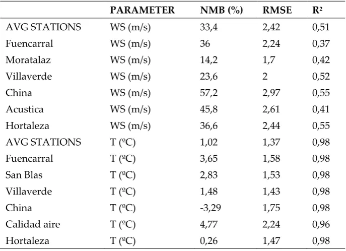
Normalized Mean Bias (NMB), Root Mean Square Error (RMSE) and Pearson's correlation coefficient (R2).
Table 2. Madrid results of the evaluation of the results of the modelling system.
PARAMETER NMB (%) RMSE R2
AVG STATIONS WS (m/s) 33,4 2,42 0,51
Fuencarral WS (m/s) 36 2,24 0,37
Moratalaz WS (m/s) 14,2 1,7 0,42
Villaverde WS (m/s) 23,6 2 0,52
China WS (m/s) 57,2 2,97 0,55
Acustica WS (m/s) 45,8 2,61 0,41
Hortaleza WS (m/s) 36,6 2,44 0,55
AVG STATIONS T (ºC) 1,02 1,37 0,98
Fuencarral T (ºC) 3,65 1,58 0,98
San Blas T (ºC) 2,83 1,53 0,98
Villaverde T (ºC) 1,48 1,43 0,98
China T (ºC) -3,29 1,75 0,98
Calidad aire T (ºC) 4,77 2,24 0,96
Hortaleza T (ºC) 0,26 1,47 0,98
The comparison between the modelled data and observed data shows that the simulated values are within the ranges of the measured data. The simulated average levels are within the inter-annual variability of the measurement, since most R2 values exceed the value of 0.5, except for wind speed (WS) at some measurement points. The statistical evaluation shows significant evidence that the applied high-resolution scale reduction procedure achieves reasonably good performance, in particular for NMB and R2 statistics. In the case of temperature the statistics are really good, outdoor temperature is a key input for energy simulations of buildings; the prediction has an error of less than 5%.
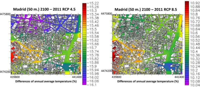
Figure 1. Madrid, 50 meters resolution. Differences between scenarios in 2100 and 2011 annual average temperature (%). RCP 4.5 scenarios to the left, RCP 8.5 right.
If we compare the maps of the climatic scenarios RCP 8.5 and RCP 4.5 we can conclude that a considerable increase in the temperature caused by the global climatic scenario RCP 8.5 is expected. In the case of the RCP 4.5 climate scenario, more important decreases are expected. The areas more affected by the decrements correspond to north zones. In the more density urban areas, strong increases are expected as a consequence of the global scenario RCP 8.5. The mean increase of the annual average temperature is 10.5 % (+1.7 ºC) for the RCP 8.5 climate scenario and decreases around 15.6 % (-2.4 ºC) for the RCP 4.5 climate scenario.
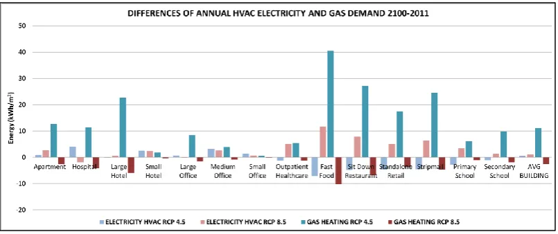
Figure 2. Differences between scenarios in 2100 and 2011 annual HVAC energy demand (electricity and gas) kWh/m2 for 14 prototypes and mean building. RCP 4.5 scenario (blue bars) and RCP 8.5 right (red bars).
The calculated monthly energy demand for space heating and cooling and outdoor temperature differences 2100-2011 (kWh/m2) for fast food restaurant with the two climate scenarios are show in Figure 3.
Figure 3. Differences between scenarios in 2100 and 2011 monthly HVAC energy demand (electricity and gas) kWh/m2 for fast food restaurant. RCP 4.5 scenario (blue bars) and RCP 8.5 right (red bars).
The increment of electricity demand per 1ºC temperature is 0.59 kWh/m2 1º with RCP 8.5 and with the RCP 4.5 the reduction is 0.21. kWh/m2 for a prototype fast food restaurant located in Madrid.
Now we are going to present the results of the electrical demand of the 94 building blocks simulated for a Madrid area of 1km by 1km. The table 3 presents the variations (%)of the annual total electricity, fans electricity, cooling electricity, heating electricity and outdoor temperature average of the 94 simulated building blocks between 2100 versus 2011 with the two climate scenarios RCP 4.5 and RCP 8.5.
Table 3. Variations on electricity demand for 2100 versus 2011 of 94 building blocks of Madrid. Climate scenarios RCP 4.5 and RCP 8.5
AVG 94 buildings blocks
of Madrid 1km x 1km area
2100 - 2011
4.5 8.5
Δ Total Electricity (%) -9.56 11.71
Δ Fans Electricity (%) -0.12 0.81
Δ Cooling Electricity (%) -25.07 26.99
Δ Heating Electricity (%) 70.28 -17.95
Δ Outdoor Temperature (%) -16.41 10.43
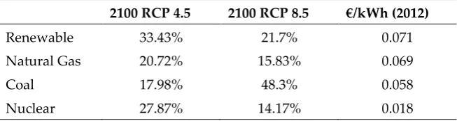
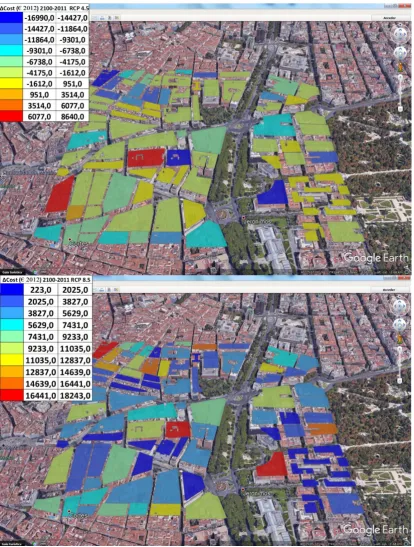
In the RCP 8.5 we can observe a very strong increment on the electricity demand for cooling the buildings (26.99 %). It is interesting to notice that increased future local temperatures translate in higher energy consumption for cooling. In the RCP 4.5 decreases of electrical consumption for cooling (-25.07%) are observed because due to very important decreases of the temperature (-16.41 %). Some buildings use electricity for heating and they will increase the heating electricity up to 70.28% for 2100 year with RCP 4.5. Under the RCP 8.5 climate scenario, electricity demand is projected to rise (11.71 %) due to cooling demand in 2100. Under the best climate scenario (RCP 4.5) electricity demand will decrease (9.56 %). Now we have calculated the cost of electricity energy demand impacts taking into account the distribution of the energy sources defined in the climate scenarios RCP 4.5 and RCP 8.5 [11]. We have considered 2012 prices of kWh published by the Spanish Commission of the Energy. The information is summarized in the Table 4.
Table 4. Energy source 2100 climate scenarios and cost of electricity.
2100 RCP 4.5 2100 RCP 8.5 €/kWh (2012)
Renewable 33.43% 21.7% 0.071
Natural Gas 20.72% 15.83% 0.069
Coal 17.98% 48.3% 0.058
Nuclear 27.87% 14.17% 0.018
2100. In RCP 4.5 some building (blue and green buildings) will save money in 2100 respect to 2011 because the decrements of the temperature. The spatial distribution of electricity demand changes is not uniform in the Madrid area and depends upon local climate and characteristics of the buildings. These kind of data could be used for specific efficiency upgrades to maximize energy demand reductions.
Figure 4. Differences between scenarios in 2100 and 2011 annual cost of electricity energy demand impacts using 50 meters spatial resolution climate data over Madrid. RCP 4.5 scenarios to the top, RCP 8.5 bottom.
4. Conclusions
In this experiment we have illustrated the impact of future climate change scenarios on energy demand for heating and cooling of buildings. Our analysis is based on the IPCC climate scenarios RCP 4.5 and RCP 8.5 focused in Madrid City. The energy consumption of heating and cooling of 14 prototype buildings and 94 blocks of real buildings in a 1km x 1km area of Madrid city during 2011 and 2100 years, were simulated using the EnergyPlus model. In this research paper, we have described a tool for the assessment of micro-coupled simulations to study the impact of climate change scenarios in the city of Madrid. This tool requires an essential key input which are the climate variables affecting the close environment of the different buildings.
A three-dimensional numerical nesting procedure was used to assess the effects of climate change using a dynamic downscaling approach to assess the effects of climate change at local scale. The model chain (tool) included a global climate model (CESM), as well as a mesoscale urban model (WRF nested with UCM of 50 to 1 km resolution) and a microscale model (MICROSYS) (CFD approach). The integrated framework allows climate and associated impacts to be projected at different spatial and temporal scales which are relevant to local/regional urban planning. Micro-level weather results were evaluated using observations from existing weather stations. The evaluation of the dynamic climate modelling system demonstrated the utility and applicability of the results. To improve the simulation tool, more validation studies comparing simulation results with field measurements are required.
The results show significant increases in heating demand in buildings in Madrid city for the climate scenario RCP 4.5 This is mainly due to substantial temperature decreases over the next 100 years and also due to the increase in cooling demand. For the energy dynamics in the buildings in Madrid studied in the case of scenario RCP 8.5, the temperature will also increase in 2100 year compared with the 2011 year. However, the increase and decrease in energy demand is different for each type of building in Madrid city. Restaurants and large hotels are those buildings mostly affected by climate change. In general, the cooling electricity of large buildings will increase more than in the case of small buildings. Results show than electric energy consumption for cooling is 26.99 % higher in RCP 8.5 2100 in comparison to 2011 year. On average the global climate for year 2100 will have an impact on a typical Madrid buildings block of 5336 euros per year following the RCP 8.5 and the RCP 4.5 will save 4100 euros per year because space cooling demand is more significant than space heating demand for Madrid buildings under the considered climate scenarios. The results indicate that the energy demand for buildings in Madrid is very sensitive to the global climate. For the general buildings, the scenario RCP 8.5 will produce more favorable climatic conditions, from the point of view of the building energy demand as it is characterized by temperature increases. In this case, because the temperature increases, cooling increments are needed to reach the comfort temperature, which are compensated by the decrease in gas consumption for heating. The results are consistent with other studies which under warmer climate conditions suggest high cooling demands [28, 29]. Other studies show trends of decreasing heating and increasing cooling demands under RCP 8.5 climate scenario [30, 31]. Last studies suggest that current carbon emissions trends most closely follow RCP 8.5 [32], where space conditioning is a major driver of the increases in electricity demand. The described tool in this contribution is very relevant when checking the final results since the conclusions can be applied to other buildings and locations. These climate impact studies contribute to find solutions that will enhance the resilience of buildings to future climate changes. The large variations between climate change and energy consumption in buildings enhance the importance of a priori assessment of climate change impacts at the local level using the state-of-the-art climate and energy modelling tools. When constructing new buildings, information from this type of studies can be used to adopt design strategies to adapt to local climatic conditions in order to optimize both heating and cooling demands in relation to climate change. Future studies may combine the influence of climate with different building designs in order to find the best solutions to minimise the heating and cooling costs of buildings.
Juan L. Pérez; writing—original draft preparation, Juan L. Pérez.; writing—review and editing, Roberto San José and Rosa Maria Gonzalez-Barras; visualization, Juan L. Pérez.; supervision, Roberto San José. All authors have read and agreed to the published version of the manuscript
Funding: This research received no external funding
Acknowledgments: The UPM authors acknowledge the computer resources and technical assistance provided by the Centro de Supercomputación y Visualización de Madrid (CeSViMa). The UPM authors thankfully acknowledge the computer resources, technical expertise and assistance provided by the Red Española de Supercomputación).
Conflicts of Interest: The authors declare no conflict of interest. References
1. Saheb, Y., Bódis, K., Szabó, S., Ossenbrink, H., & Panev, S. (2015). Energy Renovation: The Trump Card for the New Start for Europe (Report EUR 26888 EN).
2. Radhi G. H, “Evaluating the potential impact of global warming on the UAE residential buildings - A contribution to reduce the CO2 emissions,” Building and Environment, 2009, vol. 44, pp. 2451-2462. 3. Oleson, K. W., A. Monaghan, O. Wilhelmi , M. Barlage , N. Brunsell , J. Feddema , L. Hu , and D. F. Steinhoff.
Interactions between urbanization, heat stress, and climate change. Climatic Change 2010; 129, 525-541, doi:10.1007/ s10584-013-0936-8.
4. Mickley, L. J., Jacob, D. J., Field, B. D., and Rind, D. Effects of future climate change on regional air pollution episodes in the United States, Geophys. Res. Let. 2004; 31, L24103.
5. Olonscheck, M., Holsten, A., Kropp, J., 2011. Heating and cooling energy demand and related emissions of the German residential building stock under climate change. Energy Policy 39, 4795–4806.
6. Sailor D. J., “Relating residential and commercial sector electricity loads to climate: Evaluating state level
sensitivities and vulnerabilities,” Energy, vol. 26, pp. 645-657, 2001.
7. Piringer M., E. Petz, I. Groehn, and G. Schauberger, “A sensitivity study of separation distances calculated
with the Austrian Odour Dispersion Model (AODM),” Atmospheric Environment, vol. 41, pp. 725-1735, 2007.
8. Christensen J.H and O. B. Christensen, “A summary of the PRUDENCE model projections of changes in European climate by the end of this century,” Climatic Change, vol. 81, pp. 7–30, 2007.
9. Yuqing, W., et al., 2004: Regional climate modeling: progress, challenges, and prospects, J. Meteorol. Soc. Jpn. 82, pp. 1599-1628.
10. Isaac, M.,van Vuuren, D.P., 2009. Modeling global residential sector energy demand for heating and air conditioning in the context of climate change. Energy Policy 37, 507–521.
11. Ruth M and A. D. Amato, “Regional Energy Demand Responses to Climate Change: Methodology and Applications to the Commonwealth of Massachusetts,” Climatic Change, 2005, vol. 70, no. 1, pp. 175-201. 12. Rosenthal D.H., H. K. Gruenspecht, and E. A. Moran, “Effects of global warming on energy use for space
heating and cooling in the United States,” Energy J, vol. 16, pp. 77–96, 1995.
13. Belzer D.B., J. M. Scott, and R. D. Sands, “Climate change impacts on U.S. commercial building energy
consumption: An analysis using sample survey data,” Energy Sources, vol. 18, pp. 177–201, 1996.
14. Pretlove S.E.C. and T. Oreszczyn, “Climate change: Impact on the environmental design of buildings,” in
Proc CIBSE A Build Serv Eng Res Technol, 1998, vol. 19, pp. 55–58
15. Cartalis C, A. Synodinou, M. Proedrou, A. Tsangrassoulis, and M. Santamouris, “Modifications in energy
demand in urban areas as a result of climate changes: An assessment for the southeast Mediterranean
region,” Energy Conversion Manage, vol. 42, pp. 1656–1674, 2001
16. Li D.H.W, L. Yang, and J. C. Lam, “Impact of climate change on energy use in the built environment in
different climate zones –A review,” Energy, vol. 42, pp. 103-112, 2012.
17. Vuuren, D.P., Edmonds, J., Kainuma, M., Riahi, K., Thomson, A., Hibbard, K., Hurtt, G.C., Kram, T., Krey, V., Lamarque, J.F., Masui, T., Meinshausen, M., Nakicenovic, N., Smith, S.J., Rose, S.K.The representative concentration pathways: an overview. Climatic Change 109, 2011, 5‐31.
19. Riahi, S. Rose, P. Runci, R. Stouffer, D. van Vuuren, J. Weyant, T. Wilbanks, J. P. van Ypersele, and M.a
Zurek, “Towards new scenarios for analysis of emissions, climate change, impacts, and response strategies,” Intergovernmental Panel on Climate Change, 2008, Geneva, pp. 132.
20. Smith, R. J. Stouffer, A. M. Thomson, J. P. Weyant1, and T. J. Wilbanks, “The next generation of scenarios for climate change research and assessment,” Nature, vol. 463, pp. 747-756, 2010.
21. Hurrell, J. W., et al. (2013), The Community Earth System Model: A framework for collaborative research, Bull. Am. Meteorol. Soc., 94, 1339–1360.
22. Skamarock W, Klemp J, Dudhia J, Gill D, Barker D, et.al, (2008) A description of the Advanced Research WRF version 3. NCAR Tech. Note NCAR/TN-4751STR 113.
23. Kusaka, H. and Kimura, F.: Coupling a single-layer urban canopy model with a simple atmospheric model: Impact on urban heat island simulation for an idealized case, J. Appl.Meteor., 43, 1899– 1910, 2004. 24. San Jose R, Perez JL, Morant JL and Gonzales RM. Implementation of energy fluxes in EULAG with a new
3D shadow model. International Journal of Environment and Pollution (IJEP), Vol. 50, No. 1/2/3/4, 2012 25. Masson V. A physically-based scheme for the urban energy budget in atmospheric models. Boundary Layer
Meteorol. 2000; 94: 357-397.
26. San José R, J. Pérez, L. Pérez, R. González , J. Pecci, A. Garzón, and M. Palacios, “Impacts on the Urban Air Quality and Health of Global Climate Scenarios Using Different Dynamical Downscaling Approaches,”
Journal of Geoscience and Environment Protection, vol. 4, pp. 168-174, 2016.
27. Department of Energy, EnergyPlus Engineering Reference: The Reference to EnergyPlus. Calculations, Department of Energy, Washington, DC, 2010.
28. Rohdin, P., Molin, A., & Moshfegh, B. (2014). Experiences from nine passive houses in Sweden – Indoor thermal environment and energy use. Building and Environment, 71, 176–185
29. Tabatabaei Sameni, S. M., Gaterell, M., Montazami, A., & Ahmed, A. (2015). Overheating investigation in UK social housing flats built to the Passivhaus standard. Building and Environment
30. Berger, T., Amann, C., Formayer, H., Korjenic, A., Pospischal, B., Neururer, C., & Smutny, R. (2014). Impacts of climate change upon cooling and heating energy demand of office buildings in Vienna, Austria. Energy and Buildings, 80, 517–530
31. Dodoo, A., & Gustavsson, L. (2016). Energy use and overheating risk of Swedish multi storey residential buildings under different climate scenarios. Energy, 97, 534–548
32. Sanford, T., Frumhoff, P. C., Luers, A. & Gulledge, J. The climate policy narrative for a dangerously warming world. Nat. Clim. Change 4, 164–166 (2014).